


Abstract
Using the CANDELS photometric catalogs for the Hubble Space Telescope/ACS and WFC3, we identified massive evolved galaxies at 3 < z < 4.5 employing three different selection methods. We find the comoving number density of these objects to be ∼2 × 10⁻⁵ and 8 × 10⁻⁶ Mpc−3 after correction for completeness for two redshift bins centered at z = 3.4, 4.7. We quantify a measure of how much confidence we should have for each candidate galaxy from different selections and what the conservative error estimates propagated into our selection are. Then we compare the evolution of the corresponding number densities and their stellar mass density with numerical simulations, semianalytical models, and previous observational estimates, which shows slight tension at higher redshifts as the models tend to underestimate the number and mass densities. By estimating the average halo masses of the candidates (Mh ≈ 4.2, 1.9, and 1.3 × 10¹² M⊙ for redshift bins centered at z = 3.4, 4.1, and 4.7), we find them to be consistent with halos that were efficient in turning baryons to stars, relatively immune to the feedback effects, and on the verge of transition into hot-mode accretion. This can suggest the relative cosmological starvation of the cold gas followed by an overconsumption phase in which the galaxy rapidly consumes the available cold gas as one of the possible drivers for the quenching of the massive evolved population at high redshift.
Export citation and abstract BibTeX RIS
1. Introduction
In the standard ΛCDM paradigm, most of the mass in the universe resides in structures known as dark matter halos. These provide the gravitational well within which cold gas collapses, forms stars, and, at a larger scale, forms progenitors of the galaxies we observe today (e.g., White & Rees 1978; Fall & Efstathiou 1980; Blumenthal et al. 1984; Frenk & White 2012; Wechsler & Tinker 2018). The dark matter halo itself forms from the gravitational collapse of initial perturbations in the density field at the very early universe (e.g., van Albada 1960, 1961; Peebles 1970; White 1976). The emergence of the hierarchical model of structure formation (Press & Schechter 1974; Gott et al. 1975; White & Rees 1978) supported by cosmological hydrodynamical simulations and semianalytical models suggests a bottom-up scenario, in which massive halos formed from a sequence of mergers (so-called merger trees) and mass accretion, as opposed to initial rapid collapse models (e.g., White & Frenk 1991; Navarro & Benz 1991; Katz et al. 1992; Kauffmann et al. 1993; Lacey & Cole 1993; Somerville & Primack 1999). Discovery of very massive galaxies at high redshifts ( ), which constitute most of the luminous baryonic component inside the dark matter halos, however, suggests a rapid buildup of the bulk of their stellar mass at z > 2, with intense star formation activity at early times. Submillimeter observations further confirm the starburst populations with star formation rates (SFRs) exceeding hundreds of solar masses per year (e.g., Blain et al. 2002; Capak et al. 2008; Marchesini et al. 2010; Smolčić et al. 2015). There have been many recent spectroscopic confirmations of such sources at high-redshift galaxies experiencing suppressed star formation activity (e.g., Belli et al. 2014, 2017b, 2017a, 2019; Whitaker et al. 2014; Newman et al. 2015; Glazebrook et al. 2017; Newman et al. 2018; Schreiber et al. 2018; Forrest et al. 2020; Tanaka et al. 2019; Valentino et al. 2020). To use these systems to constrain galaxy formation and evolution scenarios and study feedback and quenching mechanisms at early times requires a robust photometric selection of these objects followed by deep spectroscopic observations.
Searching for massive evolved galaxies at high redshifts is challenging due to the faint nature of these galaxies and their small number density, requiring multiwaveband deep imaging data over large areas. The Cosmic Assembly Near-infrared Deep Extragalactic Legacy Survey (Grogin et al. 2011; CANDELS; Koekemoer et al. 2011) is a treasury program on the Hubble Space Telescope (HST) providing deep multiwaveband imaging data, allowing detection of such massive systems when the universe was 1–2 Gyr old. Studying these massive systems with relatively small star formation activity can help us understand the mass assembly of galaxies at very early times and estimate the baryonic content of the universe that turned into stars, as well as study the primary physical processes responsible for the rapid star formation activity experienced by progenitors of these galaxies. Also, since the universe has a colder gas reservoir at an early time, we would expect a high level of star formation that persists longer. Therefore, the low star formation activity of the massive evolved galaxies requires an explanation of the physical mechanisms involved in quenching seen in these galaxies and perhaps other mechanisms for maintaining their low star formation activity. Measuring the evolution of the number/stellar mass density of these systems with a relatively high stellar mass (i.e.,  ) and low specific SFR (sSFR; i.e., sSFR
  yr−1 for z ∼ 3 targets) will shed light on some of the outstanding questions regarding the early evolution of galaxies.
Over the last two decades, different techniques have been developed to identify different populations of high-redshift galaxies (Cimatti et al. 2002; Roche et al. 2002; Daddi et al. 2004; Mobasher et al. 2005; Reddy et al. 2005; Daddi et al. 2007; Grazian et al. 2007; Lane et al. 2007; Rodighiero et al. 2007; Wiklind et al. 2007; Fontana et al. 2009; Mancini et al. 2009; Williams et al. 2009; Caputi et al. 2012; Arnouts et al. 2013; Whitaker et al. 2013; Barro et al. 2014; Nayyeri et al. 2014; Straatman et al. 2014; Fumagalli et al. 2016; Pacifici et al. 2016; Siudek et al. 2017; Fang et al. 2018; Merlin et al. 2018; Carnall et al. 2018, 2019b, 2020). However, different methods optimized to find the same population of high-redshift galaxies often result in different samples with varying levels of contamination when applied to the same data set.
This paper compares different techniques used for the selection of massive evolved galaxies at high redshifts. Here we apply these methods to the same data set and compare the results. We then quantify the degree of confidence for each of the detected sources to be a member of the galaxy population in question.
In Section 2, we present the data. Different selection techniques are introduced in Section 3 and applied to the CANDELS data to identify massive evolved galaxies. In Section 4, we compare these methods and analyze the effect of photometric errors on each of them. In Section 5, we compare the number and stellar mass densities of the quiescent galaxies with previous values reported from observations and cosmological simulations. We discuss our results in Section 6. We present our final catalog of massive evolved galaxies in the Appendix.
We assume a standard cosmology with H0 = 70 km s−1 Mpc−1, Ωb = 0.0486, Ωm = 0.3089, and ΩΛ = 0.7 from the Planck Collaboration et al. (2016), unless stated otherwise. All magnitudes are in the AB system, where  (Oke & Gunn 1983).
2. Data
We use the latest photometric catalogs from CANDELS with consistent multiwaveband photometry and physical parameters for all galaxies to the flux limit of the sample.14 Details about the selection and photometry at different bands were carried out for all of the CANDELS fields, consisting of GOODS-South (Guo et al. 2013; Santini et al. 2015), UDS (Galametz et al. 2013; Santini et al. 2015), COSMOS (Nayyeri et al. 2017), EGS (Stefanon et al. 2017), and GOODS-North (Barro et al. 2019). These catalogs contain observed photometry from the UV to near- (NIR) and mid-infrared (MIR) wavelengths in many broadband and narrowband filters (Table 1), as well as inferred physical parameters.
Table 1. The Observed Bands from the UV-to-NIR SEDs of Galaxies across the Five CANDELS Fields
| Field | Filter Set |
|---|---|
| GOODSS (Guo et al. 2013) | Blanco/CTIO U, VLT/VIMOS U, |
| HST/ACS F435W, F606W, F775W, F814W, F850LP, | |
| HST/WFC3 F098M, F105W, F125W, F160W, | |
| VLT/ISAAC Ks, VLT/Hawk-I Ks, | |
| Spitzer/IRAC 3.6 μm, 4.5 μm, 5.8 μm, 8.0 μm | |
| GOODSN (Barro et al. 2019) | KPNO U, LBC U, |
| HST/ACS F435W, F606W, F775W, F814W, F850LP, | |
| HST/WFC3 F105W, F125W, F140W, F160W, F275W, | |
| MOIRCS K, CFHT Ks, | |
| Spitzer/IRAC 3.6 μm, 4.5 μm, 5.8 μm, 8.0 μm | |
| UDS (Galametz et al. 2013) | CFHT/MegaCam u, Subaru/Suprime-Cam B, V, Rc, i' , z' , |
| HST/ACS F606W, F814W, HST/WFC3 F125W, F160W, | |
| VLT/Hawk-I Y, Ks, | |
| WFCAM/UKIRT J, H, K, | |
| Spitzer/IRAC 3.6 μm, 4.5 μm, 5.8 μm, 8.0 μm | |
| EGS (Stefanon et al. 2017) | CFHT/MegaCam U*, g' , r' , i' , z' , |
| HST/ACS F606W, F814W, HST/WFC3 F125W, F140W, F160W, | |
| Mayall/NEWFIRM J1, J2, J3, H1, H2, K, | |
| CFHT/WIRCAM J, H, Ks, | |
| Spitzer/IRAC 3.6 μm, 4.5 μm, 5.8 μm, 8.0 μm | |
| COSMOS (Nayyeri et al. 2017) | CFHT/MegaCam u*, g*, r*, i*, z*, |
| Subaru/Suprime-Cam B g+, V, r+, i+, z+, | |
| HST/ACS F606W, F814W, HST/WFC3 F125W, F160W, | |
| Subaru/Suprime-Cam IA484, IA527, IA624, IA679, IA738, IA767, IB427, | |
| IB464, IB505, IB574, IB709, IB827, NB711, NB816, | |
| VLT/VISTA Y, J, H, Ks, Mayall/NEWFIRM J1, J2, J3, H1, H2, K, | |
| Spitzer/IRAC 3.6 μm, 4.5 μm, 5.8 μm, 8.0 μm | |
Download table as: ASCIITypeset image
The optical (HST/ACS) and NIR (HST/WFC3) data were consistently combined with the MIR data (Spitzer/IRAC) and ground-based observations. For each of the CANDELS fields, the photometric catalogs were selected in the HST/WFC3 F160W band using SExtractor (Bertin & Arnouts 1996). For low-resolution images, Template FITting (Tfit; Laidler et al. 2007) was performed to smooth the high-resolution image to low resolution and fit the best flux consistent with the HST data. A template is created by Tfit using prior information on the position and light distribution profile of sources in high resolution to more robustly measure photometries from the lower-resolution data. Table 2 lists the limiting magnitudes and survey areas covered for each of the CANDELS fields.
Table 2. The Survey Area and WFC3 F160W Limiting Magnitude for Different CANDELS Fields
| Field | Area (arcmin2) | F160W 5σ Limiting Magnitude (AB) |
|---|---|---|
| GOODS-North | 170 | 27.80 |
| GOODS-South | 170 | 27.36 |
| COSMOS | 216 | 27.56 |
| UDS | 202 | 27.45 |
| EGS | 206 | 27.60 |
Download table as: ASCIITypeset image
In this study, we use an improved version of the original Dahlen et al. (2013) photometric redshifts. The new catalogs are based on the probability density functions (PDFs) measured by six groups using different template-based methods applied to the CANDELS photometric catalogs. The methods are different in either their choice of parameters or the code used. The PDFs from different groups were corrected and optimized for bias (optimal shift) and variance (optimal scaling of the width of the PDF). After recalibration, the PDFs were combined based on the minimum Frechet distance (Alt & Godau 1995), which tracks the similarity between any pair of PDF curves among the independent photo-z PDFs (analogous to the median of a set of numbers). The final catalog consist of the spectroscopic/3D-HST grism redshifts and the combined photometric redshifts (D. Kodra et al. 2020, in preparation). The point estimate redshifts used in this work show a normalized median absolute deviation of σNMAD ∼ 0.02. The stellar masses were measured through spectral energy distribution (SED) fitting by keeping redshifts at their best values.
3. Selection Methods
Here we use a combination of several NIR selection techniques to identify massive quiescent galaxies at a redshift of  in the CANDELS fields. This is the redshift interval in which most of the galaxies exist; however, the full sample of galaxies is at a redshift of
  . We define the massive quiescent population as those with
  and
and  Gyr−1, in which tH(z) is the age of the universe at redshift z in Gyr. The results are cross-compared and used to compile a reliable catalog for the study of the number density and mass function of these systems in the redshift range mentioned. This comparison also allows a better understanding of the strengths and shortcomings of each method.
First, we use the color selection technique based on rest-frame or observed colors for classification. Then, we explore selection methods based on the inferred physical properties of galaxies from their best-fit model SEDs.
A serious source of uncertainty in these techniques is the choice of the somewhat subjective parameters that could significantly affect the outcome. These include the signal-to-noise ratio (S/N) in the flux in a particular band, color cuts in the color space occupied by galaxies, flux limits, and parameters used to generate template SEDs. Galaxies that are close to the decision boundaries are most likely to be affected by the choice of these parameters. Therefore, to minimize the effect of these cuts for each technique, we define a likelihood function between zero and 1 that identifies the likelihood that a given galaxy is a real member of the massive quiescent population within our specified redshift range. We then consistently combine all of these measures to find a final value associated with individual galaxies to quantify the degree of confidence for each selection method and compare different galaxies resulting from a particular selection. Then, we estimate the uncertainty in number/stellar mass density measurements coming from the selection thresholds. We refer the reader to the Appendix for more details. Following this procedure, we select 5%–10% more candidates than using a step function selection that misses galaxies close to the selection boundary. This difference is significant enough to affect the measurement of their number and mass densities. In the following section, we describe each selection method.
3.1. Rest-frame UVJ Selection
This method uses the rest-frame U, V, and J bands to select the quiescent population, as the rest-frame U − V probes the prominent Balmer break (3646 Å) seen in poststarbursts. The V − J color is used to break the degeneracy between dusty star-forming and quiescent galaxies. We can classify galaxies using a color cut that separates the quiescent and star-forming regions in the UVJ plane. This method has been developed and extensively used for classifying galaxies in photometric surveys (e.g., Labbé et al. 2005; Wuyts et al. 2007; Williams et al. 2009; Arnouts et al. 2013; Whitaker et al. 2013; Barro et al. 2014; Straatman et al. 2014; Fumagalli et al. 2016; Siudek et al. 2017; Fang et al. 2018). However, measuring UVJ colors for galaxies at high redshifts is challenging, making the selection less reliable. A typical method to infer rest-frame UVJ colors is from the best-fit model SED. The model SEDs are generally built assuming a τ model star formation history (SFH), which also becomes less reliable at high redshifts, since the galaxy model needs more time to evolve into the quiescent regions (Merlin et al. 2018) and more generally suffers from other uncertainties associated with SED fits used to infer rest-frame colors. Therefore, the boundaries of the UVJ criteria are modified at different redshift bins (Whitaker et al. 2013). However, this can introduce contamination from the dusty star-forming galaxies, given the similarity of their rest-frame U − V color. Nevertheless, the overlap in the wavelength coverage, including medium-band data, can ameliorate some of these problems when selecting high-z galaxies (e.g., Spitler et al. 2014).
To measure the rest-frame UVJ colors, we employ the prescription described by Wolf et al. (2003) for the COMBO-17 survey, where the rest-frame colors are estimated from the best-fit template SED. Rest-frame UVJ colors can also be measured by interpolating the observed bands that track the redshifted UVJ (e.g., Rudnick et al. 2003; Taylor et al. 2009; Williams et al. 2009). In the latter case, data from many bands outside of the UVJ region of the spectra are left unused, while in constraining the best-fit model SED, these data are beneficial (Brammer et al. 2011). We will further investigate the effect of the SFHs on the UVJ colors from the best-fit SEDs when analyzing the effects of the photometric uncertainties in Section 4.
We combine the selection criteria on the rest-frame UVJ plane employed in Muzzin et al. (2013), Whitaker et al. (2012), and Straatman et al. (2014) in Figure 1. We define the grading scheme by giving a weight to individual galaxies based on their distance from the boundary defined in Table 7. The combination of these selections is done by finding the likelihood that each galaxy is a member of the union of selected populations from different criteria. To find the rest-frame UVJ colors of CANDELS galaxies, we use the Le Phare SED fitting code (Arnouts et al. 1999; Ilbert et al. 2006) with the standard libraries defined in Table 3 (Chartab et al. 2020).
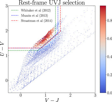
Figure 1. The rest-frame UVJ plane and colors from the best-fit models for every galaxy are shown. The artificial patterns seen are from the limited number of models that do not span the total dynamic range of the UVJ colors of galaxies. Also, since we have imposed another criterion on the F125W band, we do not select the low-z dusty solution counterparts. The color bar shows the likelihood grading for each selection. Redder data points are more likely to be quiescent. The likelihoods are assigned based on the prescription defined in the Appendix.
Download figure:
Standard image High-resolution imageTable 3. The Range of the Parameter Used in the Le Phare Code for Exponentially Declining SFH, as Well as the IMF and Dust Attenuation Law Used for Fitting All CANDELS
| SPS Model | τ Gyr | E(B − V) | IMF | Dust Attenuation Law | Metallicity |
|---|---|---|---|---|---|
| BC03 (Bruzual & Charlot 2003a) | (0.01, 30) | (0, 1.1) | Chabrier (2003) | Calzetti et al. (2000) | {0.02, 0.008, 0.004} |
Download table as: ASCIITypeset image
In addition to the criteria on the UVJ plane, we impose a mild detection constraint on the observed J band (S/N > 2), which probes blueward of the Balmer break for the highest redshift bins. This reassures that the break lies redward of the J band, reducing the contamination from low-z interlopers. The results are presented in Figure 1.
3.2. Observed Color Selection
The most commonly used methods for identifying the population of high-redshift galaxies are variations of the dropout technique, based on the observed colors of galaxies. This uses well-known features in the galaxy SEDs and follows them as they move to redder passbands when the galaxy is redshifted. Examples of this are the Lyman-break features used for the selection of UV-bright Lyman-break galaxies (Steidel & Hamilton 1993; Steidel et al. 1995; Steidel et al. 2003; Reddy et al. 2005; Stark et al. 2010; Bouwens et al. 2011; Bouwens et al. 2014; Roberts-Borsani et al. 2016; Oesch et al. 2016) and evolved systems using Balmer-break features (Cimatti et al. 2002; Roche et al. 2002; Franx et al. 2003; van Dokkum et al. 2003; Daddi et al. 2004, 2007; Reddy et al. 2005; Mobasher et al. 2005; Lane et al. 2007; Rodighiero et al. 2007; Wiklind et al. 2007; Caputi et al. 2012; Nayyeri et al. 2014; Girelli et al. 2019).
This technique uses the fact that magnitudes and colors are sensitive to redshift and the shape of their SEDs, which follows the physical properties of their stellar population and interstellar medium. For example, for poststarburst galaxies, we can use Balmer-break features from the 3648 Å Balmer limit. Therefore, the observed colors can help us find the candidate galaxies directly from photometric measurements using a few photometric bands. For the redshift range of interest here, Balmer-break features redshift toward NIR wavelengths.
We use the observed colors to select candidates in the CANDELS fields with the color selection criteria from Nayyeri et al. (2014) in Figure 2. This selection was initially developed by finding the color criteria in the color–color space for a sample of old (low-z) quiescent, dusty starburst, and poststarburst populations using Bruzual & Charlot (2003a) stellar population synthesis evolutionary tracks and considering intergalactic medium (IGM) absorption following Madau (1995). In the redshift range of interest ( ), H − K color will constrain the presence of the Balmer break, accompanied by a Y − J or J − H constraint that can discriminate between dusty starburst and quiescent galaxies. Also, we impose a nondetection requirement on the U and B bands, since they fall blueward of the break. By doing this, we reduce the contamination from the low-redshift interlopers. Another likely source of contamination is due to the absence of nebular emission lines. These affect the selection based on broadband photometry because they can mimic a Balmer-break feature, which can mislead the classification scheme (see Nayyeri et al. 2014; Straatman et al. 2014; Merlin et al. 2018). To minimize the effect of these lines, we perform the SED fitting procedure described in Section 3.3 using libraries with and without the nebular line emissions.
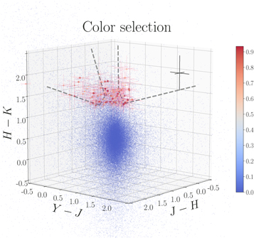
Figure 2. Observed color selection based on the criteria in Nayyeri et al. (2014) in three dimensions. The gray dashed line shows these selection boundaries on the 2D planes of the colors. The redness of the points indicates the degree to which each galaxy is a member of the quiescent population. The error bars are plotted for sources with a likelihood higher than 0.5. The likelihoods are assigned based on the prescription defined in the Appendix.
Download figure:
Standard image High-resolution imageWe assign likelihoods to the selected sources based on their proximity to the selection boundaries to reduce the dependence on the chosen selection boundaries (more details are presented in the Appendix). The final likelihood will be the average likelihood for all of the realizations of a galaxy within its error bars, which we call Balmer Break Galaxy (BBG) likelihood (Section 4.2).
3.3. Selection Based on SED Fitting
Here we discuss another method used for finding quiescent candidates based on the inferred physical properties measured from their SEDs. The advantage of this method is that it makes use of all of the photometric data available and, therefore, imposes stronger constraints on the selection process. Furthermore, it predicts the physical parameters for each galaxy. The disadvantage is that the method is model-dependent and based on the SFH and extinction used to generate SED templates (Grazian et al. 2007; Fontana et al. 2009; Pacifici et al. 2016; Carnall et al. 2018; Merlin et al. 2018, 2019; Carnall et al. 2019b). We fit template SEDs for the candidates in the range 2.8 < zphot < 5.4 with masses larger than 1010 M⊙ using CANDELS photometric and spectroscopic redshifts (where available) and a catalog of the physical properties. We rely only on the mass measurements, since the stellar masses are less susceptible to the parameters chosen in the template libraries of galaxies, particularly the SFH used for SED fitting (compared to the inferred SFRs; Papovich et al. 2001; Shapley et al. 2001; Wuyts et al. 2009; Muzzin et al. 2009; Mobasher et al. 2015). However, the presence of the nebular lines can affect stellar mass measurements. Hence, we treat the stellar mass as a free parameter (although we made a prior mass selection on the subsample) when fitting the subsample photometric measurements to keep the stellar mass uncertainty of this type limited to the initial selection.
We find the physical properties using the Bayesian Analysis of Galaxies for Physical Inference and Parameter EStimation (Bagpipes), a Bayesian SED fitting code (see Carnall et al. 2018). Bagpipes uses the 2016 version of Bruzual & Charlot (2003a) and Multinest (Feroz & Hobson 2008; Feroz et al. 2009) for a multimodal nested sampling algorithm (Skilling 2006). The multimodal nested sampling algorithm employed is a huge improvement over a simple χ2 fit, which is incapable of producing a reliable error estimate. Moreover, the Markov Chain Monte Carlo (MCMC) algorithm employed in some SED fitting procedures for finding the posterior of the physical properties can be problematic when sampling from a multimodal posterior. These include models with a large degeneracy, which is often the case when modeling a complex system such as a galaxy under large photometric uncertainties.
We fixed redshifts to their photo-z and, where available, spec-z values. We built separate model libraries based on three prescriptions for SFHs: exponentially declining, top-hat, and double power-law forms (Behroozi et al. 2013b) assuming a Chabrier (2003) initial mass function (IMF); dust attenuation based on Calzetti et al. (2000); and IGM absorption from Inoue et al. (2014), which is a revised version of the Madau (1995) model. It is known that the presence of the nebular lines can mimic a Balmer break-like feature in broadband photometry. Therefore, for controlling their effects on the physical properties and consequently, the selection made based on them, we run the code with and without the nebular emission (since the target population is expected to have little to no nebular emission). The priors used for the physical parameters in the SED fitting are listed in Table 4. We then find the posterior distribution for each model parameter. Following Carnall et al. (2018), we define ψSFR as the ratio of the SFR at any given time (SFR(t)) to the average SFR over the age of a given galaxy ( ),
),
and we define the quiescent population as those with  less than 0.1 at the observed age of the galaxy. In other words, the quiescent galaxies are those with an average SFR over the last 100 Myr of less than 10% of the average SFR over its lifetime.
Table 4. Priors Used for Different Free Physical Parameters and the Fixed Parameters Used in the Fit
| SFH | Free Parameter | Prior | Limits | Fixed Parameter | Value |
|---|---|---|---|---|---|
| AV1 | Uniform | (0, 2) | SPS models | BC03 | |
| Double power law |
 2
2
|
Uniform | (1, 13) | IMF | Chabrier (2003) |
 3
3
|
Uniform | (0.2, 2.5) | zobs |

|
|
![${\rm{SFR}}{(t)=C{[(t/\tau )}^{\alpha }+{(t/\tau )}^{-\beta }]}^{-1}$](https://content.cld.iop.org/journals/0004-637X/897/1/44/revision1/apjab96c5ieqn15.gif)
|
 4
4
|
Uniform | (0, 
|
 5
5
|
−3 |
| α6 | Logarithmic | (10−2, 103) | |||
| β7 | Logarithmic | (10−2, 103) | |||
| AV | Uniform | (0, 2) | SPS models | BC0312 | |
| Exponentially declining |

|
Uniform | (1, 13) | IMF | Chabrier (2003) |

|
Uniform | (0.2, 2.5) | zobs |

|
|
|
 8
8
|
Uniform | (0.05, 10) |

|
−3 |
| Age | Uniform | (0, 
|
|||
| AV | Uniform | (0, 2) | SPS models | BC03 | |
| Top hat |

|
Uniform | (1, 13) | IMF | Chabrier (2003) |

|
Uniform | (0.2, 2.5) | zobs |

|
|
![${\rm{SFR}}(t)=\left\{\begin{array}{lc}C & t\in [{\mathrm{Age}}_{\min },{\mathrm{Age}}_{\max }]\\ 0 & \mathrm{otherwise}\end{array}\right.$](https://content.cld.iop.org/journals/0004-637X/897/1/44/revision1/apjab96c5ieqn29.gif)
|
Age 9
9
|
Uniform | (0, 
|

|
−3 |
Age 10
10
|
Uniform | (0,  ) ) |
|||
Notes.
1Av is the attenuation at 5500 Å. 2Mformed is the mass formed. 3 is the metallicity.
4τ is the peak time for double power-law SFH.
5
is the metallicity.
4τ is the peak time for double power-law SFH.
5
 is the ionization parameter.
6α is the rising power.
7β is the falling power.
8τ is the exponential decay timescale in τ model SFH.
9Agemin is the initial time for the top-hat SFH.
10Agemax is the final time for the top-hat SFH, and 11C is the normalization constant.
12BC03 is the stellar population synthesis at the resolution of 2003 (Bruzual & Charlot 2003b).
is the ionization parameter.
6α is the rising power.
7β is the falling power.
8τ is the exponential decay timescale in τ model SFH.
9Agemin is the initial time for the top-hat SFH.
10Agemax is the final time for the top-hat SFH, and 11C is the normalization constant.
12BC03 is the stellar population synthesis at the resolution of 2003 (Bruzual & Charlot 2003b).
Download table as: ASCIITypeset image
Carnall et al. (2018) showed that the selection criterion mentioned above is consistent with the definition proposed in Pacifici et al. (2016; see Figure 4), which is a criterion on the sSFR evolving with redshift to define the quiescent population at a given age of the universe.
The Bayesian nature of the SED fitting code allows us to have the posterior distribution for each galaxy and all parameters associated with it. Then we can apply the selection on the sample from the posterior and count the number of selected samples from the posterior versus the total count. We assign this ratio as the probability of being selected given the posterior sample. We apply the same prescription for the rest of the models employed.
We use the Bayesian evidence (marginal likelihood) on different models used for SED fitting. By doing so, we find the relative evidence for different models according to the data. The definition of the Bayesian evidence is

where D, H, and θ represent the data, hypothesis (model), and model parameters, respectively. The  is the probability of getting the data D under the assumption of the validity of a specific hypothesis H, which is the Bayesian evidence for H.
We adopt the Jeffreys criterion (Jeffreys 1961; also see Kass & Raftery 1995) for interpretation of the relative evidence (Bayes factor) calculated for each galaxy and different models. We use the same prior for fixed parameters such as redshift, and for the rest of the parameters, we use noninformative priors (Kass & Wasserman 1996) across different models. By doing so, the Bayes factor represents the posterior odds of the models, ( ). In other words, we impose no prior judgment about the validity of a certain model. Results presented in Figure 3 express that statistically; none of the models show substantially more evidence. However, the Bayes factors support models that include nebular lines and generally favor double power-law over τ models. This is consistent with Reddy et al. (2012) regarding the inability of the τ models in reproducing SFRs from UV+IR measurements in the star-forming population at higher redshifts. Pacifici et al. (2016) showed that the double power law is the best model to describe the SFHs of their samples. Carnall et al. (2019a) also confirmed that a double power-law model could produce relatively stronger evidence. As Figure 3 depicts, similar to Belli et al.'s (2019) investigation of the effect of SFH on age measurements, top-hat models generally fail to produce a comparable level of evidence from data. Therefore, we do not use the results from the top-hat models for making a selection.
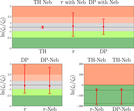
Figure 3. Bayes factor for models with different SFHs and with/without nebular emission for the redshift and mass-selected sample of galaxies. Here TH, τ, and DP stand for top-hat, exponentially declining, and double power-law models for SFH, respectively. The top panel shows the Bayes factor for models with and without nebular emissions, while having the same SFH. The bottom left panel shows the relative evidence for top-hat SFH to τ models and a double power law. The bottom right panel shows the relative evidence for τ models and a double power law. The data points show the median, and the error bars are the 20th and 80th percentiles of the sample. Here ζ1 and ζ2 are evidence for the top and bottom models (in each figure). The gray area shows inconclusive to weak evidence, the lighter color shows weak to moderate evidence, and the darker color shows moderate to strong evidence (Jeffreys 1961). In the case of top-hat models, there is strong evidence against the top-hat models when compared with τ and a double power law.
Download figure:
Standard image High-resolution image3.4. AGN Contamination
We cross-matched the potential candidates for high-redshift massive evolved systems with the publicly available Chandra X-ray catalogs and used the Spitzer MIPS 24 μm to detect possible dusty active galactic nuclei (AGNs). We excluded any candidates with a counterpart (shows detection) in either the X-ray or MIPS. For the X-ray catalogs, we looked for any counterparts closer than 5'', which is 10 times the resolution of the Chandra X-ray Observatory (cross-matched with Laird et al. 2009; Evans et al. 2010; Nandra et al. 2015; Xue et al. 2016; Cappelluti et al. 2016; Civano et al. 2016; Masini et al. 2018), and for MIR, we used the catalog published in Barro et al. (2019) for finding any counterpart and flux measurements in the mentioned MIR bands. About 30% of the candidates have X-ray or MIR counterparts, which were removed from the final sample.
3.5. Final Sample
To each galaxy, we assigned a likelihood measure that is the median of the likelihoods estimated for that galaxy from each of the three techniques: the UVJ selection (Section 3.1), observed color selection (Section 3.2), and SED fitting method with and without the nebular emission contribution (Section 3.3). We combine the results from the SED fitting under different assumptions using the weighted average of the likelihoods for each galaxy using the marginal likelihood calculated for a particular model as their corresponding weights. By doing this, we make sure that we have put more emphasis on likelihoods calculated from the models with higher marginal likelihoods. Then we take the median of all of these methods as our final indicator. We select the final sample as those with a median likelihood higher than 0.5. However, we use the 0.3 and 0.7 criteria as our least and most conservative samples, respectively. By using the median indicator, we limit our sample to those galaxies that were assigned by at least two of the methods mentioned to have a high likelihood of being a massive evolved galaxy. Figure 8 shows how this threshold changes the number density measurements of each selection method, as well as the median value that is taken as the final indicator. The final selected galaxies with their assigned likelihoods and estimated physical parameters are listed in Table 5. The galaxies that were selected with a median likelihood higher than 0.3 constitute the most inclusive sample and the one used for finding the upper bounds on the number/mass densities. Also, we control the possible contamination in our final sample, since we rely on the composite indicator compared to a single measure. Figure 4 shows a comparison between different selection methods and how they relate to each other (all highlighted points are galaxies in our final sample). For example, the selection in the sSFR versus Ms plane is generally consistent across different methods, since the objects with higher BBG/UVJ likelihood are close to or inside the selection boundary. For selection in the UVJ colors, we have several candidates that are far from the boundary but show a much higher BBG/SED likelihood. This shows the sensitivity of the final results to the libraries used, and by changing the SED fitting code and/or the libraries used, we are not necessarily searching through the same part of the models' parameter space. In terms of the selection based on the observed colors, we tend to have a higher UVJ/BBG likelihood, but there are a couple of candidates that show higher UVJ/SED likelihoods but fall outside of the criteria. This shows the importance of using information from other bands as well.
Table 5. Candidate Galaxies and Their Likelihood Measures from Different Methods
| Field | ID | R.A. | Decl. | BBG | UVJ | SED | M* | Age | Redshift | MIPS | X-Ray |
|---|---|---|---|---|---|---|---|---|---|---|---|
| COSMOS | 3871 | 150.0839297 | 2.2235337 | 0.13 | 0.97 | 0.99 | 10.79 | 1.61 | 2.83 | False | False |
| COSMOS | 13639 | 150.0685942 | 2.3427211 | 0.35 | 0.98 | 0.95 | 10.86 | 1.46 | 2.93 | False | False |
| COSMOS | 14284 | 150.1060909 | 2.3510462 | 0.01 | 0.88 | 0.73 | 10.29 | 1.38 | 3.51 | False | False |
| COSMOS | 14403 | 150.109033 | 2.3523803 | 0.0 | 0.91 | 0.56 | 10.45 | 1.47 | 3.73 | False | False |
| COSMOS | 14528 | 150.1033018 | 2.3536424 | 0.0 | 0.46 | 0.35 | 10.63 | 1.11 | 3.12 | False | False |
| COSMOS | 14788 | 150.0543714 | 2.356883 | 0.07 | 0.33 | 0.78 | 11.2 | 1.11 | 4.02 | False | False |
| COSMOS | 16676* | 150.0614902 | 2.3786845 | 0.01 | 0.99 | 0.56 | 11.26 | 1.26 | 4.13 | False | True |
| COSMOS | 16726 | 150.102881 | 2.3794029 | 0.01 | 0.99 | 0.56 | 11.01 | 0.87 | 3.65 | True | False |
| COSMOS | 16948 | 150.0667157 | 2.3823608 | 0.04 | 0.91 | 0.43 | 10.8 | 0.87 | 3.70 | False | False |
| COSMOS | 18735 | 150.1557627 | 2.4044776 | 0.0 | 0.46 | 0.63 | 10.27 | 1.07 | 3.30 | False | False |
| COSMOS | 19502* | 150.1308597 | 2.4135984 | 0.22 | 0.86 | 0.58 | 10.78 | 0.84 | 3.87 | False | False |
| COSMOS | 21794 | 150.1707301 | 2.4442981 | 0.1 | 0.95 | 0.54 | 10.51 | 1.32 | 3.63 | False | False |
| COSMOS | 26635 | 150.0634065 | 2.5151526 | 0.13 | 0.92 | 0.61 | 10.43 | 1.08 | 3.24 | False | False |
| COSMOS | 26858 | 150.1648286 | 2.5190274 | 0.0 | 0.47 | 0.48 | 10.28 | 1.94 | 3.08 | True | False |
| COSMOS | 27856 | 150.0823166 | 2.5345944 | 0.18 | 0.95 | 0.67 | 10.79 | 0.87 | 4.08 | True | True |
| COSMOS | 31823 | 150.0597769 | 2.2810259 | 0.0 | 0.97 | 0.41 | 10.73 | 1.52 | 3.72 | True | False |
| COSMOS | 32689 | 150.2035188 | 2.3120491 | 0.0 | 0.55 | 0.73 | 10.62 | 1.47 | 3.64 | False | False |
| COSMOS | 33389 | 150.1758211 | 2.3387828 | 0.0 | 0.91 | 0.52 | 10.37 | 0.93 | 4.46 | False | False |
| COSMOS | 33927 | 150.0539523 | 2.3578909 | 0.0 | 0.46 | 0.4 | 10.04 | 1.26 | 3.25 | False | False |
| COSMOS | 33970 | 150.0799589 | 2.3592574 | 0.0 | 0.9 | 0.35 | 10.13 | 1.04 | 4.42 | False | False |
| COSMOS | 34944 | 150.0534942 | 2.3927052 | 0.0 | 0.42 | 0.58 | 10.19 | 1.66 | 3.53 | False | False |
| COSMOS | 35033 | 150.0530481 | 2.3964053 | 0.0 | 0.34 | 0.92 | 10.23 | 1.38 | 3.67 | False | False |
| COSMOS | 35098 | 150.0530811 | 2.3992994 | 0.0 | 0.46 | 0.84 | 10.14 | 1.54 | 3.19 | False | False |
| COSMOS | 35162 | 150.0536619 | 2.4022545 | 0.01 | 0.95 | 0.71 | 10.38 | 0.92 | 4.30 | False | False |
| COSMOS | 36674 | 150.1204151 | 2.4658729 | 0.0 | 0.48 | 0.84 | 10.18 | 1.86 | 3.19 | False | False |
| COSMOS | 37304 | 150.1030456 | 2.4952038 | 0.0 | 0.93 | 0.49 | 10.16 | 1.6 | 3.57 | False | False |
| COSMOS | 38150 | 150.0825841 | 2.5312043 | 0.0 | 0.99 | 0.35 | 10.2 | 0.99 | 4.29 | False | False |
| EGS | 8 | 215.300542 | 53.051323 | 0.0 | 0.93 | 0.4 | 11.06 | 1.59 | 3.76 | True | False |
| EGS | 2922 | 214.932074 | 52.818233 | 0.0 | 0.99 | 0.46 | 10.43 | 1.39 | 3.29 | False | False |
| EGS | 6162 | 215.041352 | 52.914091 | 0.0 | 0.96 | 0.39 | 10.87 | 1.58 | 3.21 | True | False |
| EGS | 6498 | 215.065871 | 52.932958 | 0.0 | 0.76 | 0.55 | 10.53 | 1.72 | 3.45 | False | False |
| EGS | 14727* | 214.895659 | 52.856515 | 0.0 | 0.8 | 0.57 | 10.98 | 1.2 | 3.05 | True | False |
| EGS | 16431 | 215.191335 | 53.074718 | 0.0 | 0.96 | 0.5 | 10.45 | 1.09 | 3.49 | False | False |
| EGS | 21158 | 214.746219 | 52.783393 | 0.0 | 0.98 | 0.44 | 11.0 | 1.34 | 3.90 | True | False |
| EGS | 21351* | 214.673655 | 52.732542 | 0.3 | 0.96 | 0.5 | 10.59 | 0.88 | 3.61 | False | False |
| EGS | 22706 | 215.122517 | 53.058015 | 0.0 | 0.98 | 0.51 | 10.5 | 1.22 | 3.25 | False | False |
| EGS | 23036* | 214.879114 | 52.88807 | 0.0 | 0.73 | 0.46 | 10.22 | 0.98 | 3.56 | False | False |
| EGS | 23572 | 215.144538 | 53.078392 | 0.0 | 0.98 | 0.44 | 10.07 | 1.64 | 3.15 | False | True |
| EGS | 24177* | 214.866081 | 52.884232 | 0.0 | 0.92 | 0.58 | 10.98 | 1.78 | 3.42 | True | False |
| EGS | 24356+ | 214.620084 | 52.70959 | 0.06 | 0.92 | 0.47 | 10.66 | 1.53 | 3.43 | False | False |
| EGS | 24948 | 214.767294 | 52.81771 | 0.0 | 0.75 | 0.52 | 10.38 | 1.38 | 3.44 | False | False |
| EGS | 25724* | 214.997776 | 52.986129 | 0.0 | 0.96 | 0.5 | 10.6 | 1.43 | 3.80 | False | False |
| EGS | 27491+ | 214.617755 | 52.724101 | 0.56 | 0.92 | 0.46 | 10.55 | 1.18 | 3.34 | False | False |
| EGS | 29547* | 214.695306 | 52.796871 | 0.16 | 0.97 | 0.51 | 10.54 | 1.59 | 3.15 | False | False |
| EGS | 30198 | 214.966237 | 52.983055 | 0.0 | 0.49 | 0.42 | 10.03 | 1.26 | 3.01 | False | False |
| EGS | 30619 | 214.981814 | 52.991238 | 0.0 | 0.94 | 0.57 | 10.56 | 1.95 | 3.07 | False | False |
| EGS | 32592 | 215.080479 | 52.921568 | 0.0 | 0.97 | 0.53 | 10.2 | 0.97 | 4.28 | False | False |
| EGS | 33316 | 215.252837 | 53.055545 | 0.0 | 0.96 | 0.54 | 10.47 | 1.04 | 3.70 | False | False |
| EGS | 35080 | 214.922243 | 52.854748 | 0.0 | 0.79 | 0.59 | 10.53 | 0.9 | 4.00 | False | False |
| EGS | 35459 | 215.231097 | 53.079181 | 0.0 | 0.88 | 0.32 | 10.0 | 1.31 | 3.95 | False | False |
| EGS | 36375 | 214.778097 | 52.774151 | 0.0 | 0.46 | 0.34 | 10.51 | 1.6 | 3.27 | False | False |
| EGS | 38679 | 214.692609 | 52.753274 | 0.0 | 0.96 | 0.65 | 10.92 | 1.36 | 3.91 | False | False |
| EGS | 41385 | 214.701834 | 52.812333 | 0.0 | 0.35 | 0.33 | 10.37 | 0.96 | 3.63 | True | False |
| Field | ID | R.A. | Decl. | BBG | UVJ | SED | M* | Age | Redshift | MIPS | X-Ray |
|---|---|---|---|---|---|---|---|---|---|---|---|
| GOODSN | 599 | 189.22477876 | 62.12097508 | 0.0 | 0.98 | 0.37 | 10.7 | 1.3 | 3.77 | False | False |
| GOODSN | 3225 | 188.99068993 | 62.16051335 | 0.13 | 0.45 | 0.94 | 10.04 | 1.98 | 3.18 | False | False |
| GOODSN | 4004* | 189.26573822 | 62.16839485 | 0.54 | 0.77 | 0.63 | 10.31 | 1.03 | 3.81 | False | False |
| GOODSN | 4572 | 189.32906181 | 62.17385428 | 0.56 | 0.63 | 0.53 | 10.37 | 1.0 | 4.15 | True | True |
| GOODSN | 4691+ | 189.10990126 | 62.17519651 | 0.88 | 0.99 | 0.48 | 10.7 | 1.64 | 3.18 | False | False |
| GOODSN | 5059* | 189.1623096 | 62.17823976 | 0.01 | 0.98 | 0.51 | 10.79 | 1.08 | 3.69 | False | False |
| GOODSN | 5744* | 189.10012474 | 62.18362694 | 0.05 | 0.98 | 0.51 | 10.39 | 1.11 | 3.46 | False | False |
| GOODSN | 6989 | 189.22148283 | 62.19241118 | 0.48 | 0.98 | 0.98 | 10.22 | 1.65 | 2.80 | False | False |
| GOODSN | 8074 | 189.15625504 | 62.19909581 | 0.48 | 0.93 | 1.0 | 11.86 | 0.63 | 5.11 | True | False |
| GOODSN | 8109 | 189.26660705 | 62.19930947 | 0.01 | 0.47 | 0.89 | 10.63 | 1.68 | 3.41* | True | False |
| GOODSN | 9083 | 189.33429106 | 62.20610777 | 0.69 | 0.58 | 0.2 | 10.11 | 1.53 | 3.62 | True | False |
| GOODSN | 9545 | 188.98263204 | 62.20890348 | 0.16 | 0.34 | 0.36 | 10.41 | 1.42 | 4.27 | False | False |
| GOODSN | 24582 | 189.40615811 | 62.34785252 | 0.5 | 0.35 | 0.0 | 9.2 | 1.95 | 2.87 | False | False |
| GOODSN | 27305 | 189.21770656 | 62.31096041 | 0.0 | 0.98 | 0.51 | 10.18 | 2.03 | 3.01 | False | False |
| GOODSS | 2032 | 53.2293854 | −27.8977318 | 0.0 | 0.96 | 0.48 | 10.07 | 1.09 | 3.08 | False | False |
| GOODSS | 2717* | 53.1893272 | −27.8884506 | 0.0 | 0.99 | 0.48 | 10.92 | 1.48 | 3.03 | False | False |
| GOODSS | 2782* | 53.0835724 | −27.8875294 | 0.75 | 0.92 | 0.49 | 10.48 | 1.53 | 3.58 | False | False |
| GOODSS | 3912* | 53.0622215 | −27.8749809 | 0.35 | 0.89 | 0.04 | 10.17 | 1.34 | 3.90 | False | False |
| GOODSS | 4503+ | 53.1132774 | −27.869875 | 0.0 | 0.86 | 0.42 | 10.91 | 1.29 | 3.59 | False | False |
| GOODSS | 4821 | 53.0825539 | −27.866745 | 0.04 | 0.75 | 0.51 | 10.24 | 1.5 | 3.10 | False | True |
| GOODSS | 5479 | 53.0784645 | −27.8598576 | 0.83 | 0.71 | 0.26 | 11.07 | 1.15 | 3.66* | True | False |
| GOODSS | 6131 | 53.0916061 | −27.8533421 | 0.47 | 0.96 | 1.0 | 11.74 | 1.1 | 5.06 | True | False |
| GOODSS | 6235 | 53.1199837 | −27.8519554 | 0.36 | 0.32 | 0.0 | 10.19 | 1.66 | 3.50 | False | False |
| GOODSS | 7526+ | 53.0786781 | −27.8395462 | 0.25 | 0.97 | 0.44 | 10.14 | 1.32 | 3.32 | False | False |
| GOODSS | 8785* | 53.0818481 | −27.8287373 | 0.61 | 0.98 | 0.48 | 10.23 | 1.47 | 3.85 | False | False |
| GOODSS | 9209* | 53.1081772 | −27.8251228 | 0.31 | 0.63 | 0.49 | 10.65 | 1.2 | 4.49 | False | False |
| GOODSS | 12178+ | 53.0392838 | −27.7993088 | 0.87 | 0.79 | 0.04 | 10.36 | 1.62 | 3.29 | False | True |
| GOODSS | 12407 | 53.2218704 | −27.7976608 | 0.0 | 0.97 | 0.34 | 11.06 | 1.03 | 4.24 | True | False |
| GOODSS | 13299 | 53.2072105 | −27.7913475 | 0.53 | 0.43 | 0.0 | 10.22 | 0.91 | 4.05 | False | False |
| GOODSS | 16671 | 53.1901817 | −27.7691402 | 0.51 | 0.98 | 0.77 | 10.46 | 1.59 | 2.87 | False | False |
| GOODSS | 17258 | 53.1411247 | −27.7643566 | 0.31 | 0.32 | 0.0 | 10.4 | 1.31 | 4.52 | False | False |
| GOODSS | 17749* | 53.1968956 | −27.7604523 | 0.99 | 0.99 | 0.49 | 10.69 | 1.69 | 3.70 | True | False |
| GOODSS | 18180* | 53.1812248 | −27.756422 | 0.98 | 0.96 | 0.46 | 10.62 | 1.01 | 3.65 | False | False |
| GOODSS | 19883* | 53.0106544 | −27.7416039 | 0.0 | 0.97 | 0.42 | 10.87 | 0.97 | 3.57 | True | True |
| GOODSS | 20111 | 53.0944252 | −27.7392502 | 0.0 | 0.32 | 0.56 | 10.82 | 1.08 | 3.13 | True | False |
| GOODSS | 22085* | 53.0738754 | −27.7221718 | 0.0 | 0.92 | 0.48 | 10.36 | 1.17 | 3.47 | False | False |
| GOODSS | 32527 | 53.0305367 | −27.7529354 | 0.0 | 0.96 | 0.35 | 10.48 | 0.83 | 4.28 | True | False |
| UDS | 164 | 34.3170586 | −5.2759099 | 0.0 | 0.44 | 0.38 | 10.46 | 0.92 | 3.53 | False | False |
| UDS | 416 | 34.5199471 | −5.2747688 | 0.0 | 0.98 | 0.46 | 11.39 | 1.33 | 3.38 | True | False |
| UDS | 635 | 34.5062943 | −5.273128 | 0.0 | 0.99 | 0.53 | 11.0 | 0.92 | 4.14 | False | False |
| UDS | 918 | 34.2661095 | −5.2721262 | 0.0 | 0.77 | 0.44 | 10.88 | 1.09 | 3.17 | True | False |
| UDS | 1244* | 34.2894669 | −5.269805 | 0.32 | 0.89 | 0.01 | 10.77 | 0.99 | 3.79 | False | False |
| UDS | 1408 | 34.5122528 | −5.2688479 | 0.0 | 0.96 | 0.49 | 10.77 | 0.98 | 4.16 | False | False |
| UDS | 2571* | 34.290432 | −5.2620749 | 0.7 | 0.8 | 0.08 | 10.52 | 1.39 | 3.70 | False | False |
| UDS | 3752 | 34.5192871 | −5.2553701 | 0.0 | 0.73 | 0.52 | 10.1 | 1.5 | 3.11 | False | False |
| UDS | 4319 | 34.4653702 | −5.2520308 | 0.23 | 0.99 | 0.51 | 11.69 | 0.89 | 4.48 | True | False |
| UDS | 4332+ | 34.4656906 | −5.2519188 | 0.01 | 0.93 | 0.57 | 10.98 | 1.7 | 3.18 | True | False |
| UDS | 5256 | 34.2441864 | −5.2458172 | 0.0 | 0.34 | 0.89 | 10.89 | 1.86 | 3.31 | False | False |
| UDS | 6218 | 34.3409538 | −5.2405558 | 0.61 | 0.76 | 0.01 | 10.89 | 0.93 | 4.07 | False | False |
| UDS | 7520* | 34.2558746 | −5.23383 | 0.57 | 0.96 | 0.46 | 11.1 | 1.48 | 3.17 | True | False |
| UDS | 7779+ | 34.2588844 | −5.2323041 | 0.54 | 0.48 | 0.29 | 10.66 | 1.75 | 3.14 | False | False |
| UDS | 8682+ | 34.2937317 | −5.2269621 | 0.82 | 0.92 | 0.26 | 10.44 | 1.58 | 3.46 | False | False |
| UDS | 13988 | 34.3857307 | −5.1989851 | 0.36 | 0.05 | 0.63 | 11.45 | 1.95 | 3.03 | True | False |
| UDS | 15748 | 34.5302429 | −5.1890779 | 0.0 | 0.46 | 0.36 | 11.26 | 2.05 | 3.08 | True | False |
| UDS | 17344 | 34.3231277 | −5.179821 | 0.35 | 0.16 | 0.44 | 10.88 | 1.87 | 3.03 | True | False |
| UDS | 17790 | 34.5422859 | −5.1774998 | 0.34 | 0.33 | 0.0 | 10.54 | 1.58 | 3.31 | True | False |
| UDS | 18672 | 34.5668411 | −5.1726952 | 0.92 | 0.51 | 0.0 | 10.32 | 1.32 | 3.79 | False | False |
| UDS | 19849 | 34.3381882 | −5.1661878 | 0.07 | 0.98 | 0.41 | 10.41 | 1.66 | 3.53 | True | False |
| UDS | 20843* | 34.4961014 | −5.161037 | 0.64 | 0.65 | 0.19 | 10.76 | 0.88 | 3.74 | False | False |
| UDS | 22354 | 34.4276466 | −5.1524191 | 0.72 | 0.38 | 0.03 | 10.93 | 1.9 | 3.15 | False | False |
| UDS | 23628* | 34.2425995 | −5.1430721 | 0.97 | 0.63 | 0.21 | 10.73 | 0.83 | 4.25 | False | False |
| UDS | 24501 | 34.5228386 | −5.1288252 | 0.0 | 0.82 | 0.34 | 10.43 | 1.55 | 3.40 | False | False |
| UDS | 24734 | 34.5229988 | −5.1295991 | 0.0 | 0.88 | 0.49 | 10.36 | 1.55 | 3.47 | False | False |
| UDS | 25688* | 34.5265884 | −5.1360388 | 0.25 | 0.99 | 0.53 | 11.21 | 1.33 | 3.08 | False | False |
| UDS | 25893* | 34.3996353 | −5.1363459 | 0.08 | 0.99 | 0.55 | 11.05 | 1.24 | 4.49 | False | False |
| UDS | 32698 | 34.5237198 | −5.1804299 | 0.0 | 0.36 | 0.61 | 10.99 | 1.29 | 4.30 | True | False |
| UDS | 35635 | 34.3170319 | −5.127574 | 0.0 | 0.93 | 0.36 | 10.58 | 1.36 | 3.72 | False | True |
Note. The asterisks and plus signs next to the IDs show the candidates found in the primary and secondary samples reported in Merlin et al. (2019), respectively. The asterisk next to the redshift indicates those with available spectroscopic redshifts. Here BBG, UVJ, and SED stand for the likelihood based on the observed color, UVJ, and SED fitting, respectively. The MIPS and X-ray columns correspond to the detection in the MIPS 24 μm and X-ray. Here M* is  , and age is the age of the candidate galaxy in Gyr. The galaxies that show a detection in the MIPS 24 μm and X-ray are excluded from the number/stellar mass density measurements (i.e., Figure 9).

Figure 4. The top panel shows the sSFR vs. Ms (from Bagpipes), the bottom left panel shows the rest-frame UVJ colors (from Le Phare), and the bottom right panel shows the observed colors for the candidate galaxies. The gray points are the CANDELS galaxies (with  ), and the candidates are color-coded with three assigned likelihoods. The green, blue, and red color scales reflect the likelihood measured based on UVJ, SED, and the observed colors, respectively. In order to show the contrast in different selections, we plotted likelihoods on top of each other. So, those that have two colors show a high likelihood in two methods, and from those, the ones that also fall inside the respective criteria show a higher likelihood in all of the mentioned methods. The shaded area shows the selection in the corresponding plane with the same color code as mentioned. In the top panel, a different limiting sSFR for SED-based selection is shown at different redshifts.
Download figure:
Standard image High-resolution image4. Photometric Uncertainty
All of the methods discussed in the previous section are sensitive to uncertainties in photometry at different levels. To quantify the sensitivity of each of the selection methods to photometric uncertainties, we use the Monte Carlo resampling and produce different realizations of each galaxy's photometries. We quantify the confidence level for each candidate galaxy selected from different methods and the error estimates that propagated into the selections.
Assuming a Gaussian error distribution for each band, we produce realizations for each galaxy by perturbing the photometric measurements within their assigned uncertainties. In other words, we build a bootstrap-resampled ensemble of the photometric measurement distribution of a galaxy. Then we perform the methods for selecting candidate galaxies and study how these perturbations affect our selections and how sensitive the selected sample is to changes in photometric measurements within their uncertainties. In the case of the selection based on the observed color technique, we only look at several bands, so the uncertainties on the other bands (not used in the selection) are not crucial, but in the case of the UVJ and SED, we use all of the photometric data, which means that the uncertainties in every band can potentially be imperative.
4.1. Uncertainty of Selection Based on UVJ
Here we consider the effect of the photometric uncertainties in finding UVJ colors and how that could affect the final selected sample. We first choose a subset of the selected galaxies, construct 50 realizations of each, and run SED fitting on the resampled galaxies. Then we quantify how these uncertainties propagate into our inferred rest-frame colors and how they change the result from the UVJ selection in Section 3.1.
Figure 5 shows the effect of photometric uncertainty on the UVJ selection. It is clear how the choice of the SFH and whether to include the nebular emissions is pivotal in selecting the quiescent population. We find the UVJ colors from the Bagpipes SED fitting code, since we are interested in understanding the effect of the photometric uncertainty on the inference from the SED, which makes a Bayesian posterior estimate more reliable given the clear uncertainty definition based on the posterior. For all but a small subset of galaxies fitted with τ models and nebular lines, the posterior UVJ of the resampled galaxies falls around the posterior from the true photometry with considerable scatter. For a small subset of galaxies (five out of 28) fitted with τ models, the locus of the posterior varies dramatically and with higher scatter than the posterior UVJ from the true photometry. The double power-law model is found to be more immune to the photometric uncertainties, as is also the case for the physical parameters used in SED-based selection.
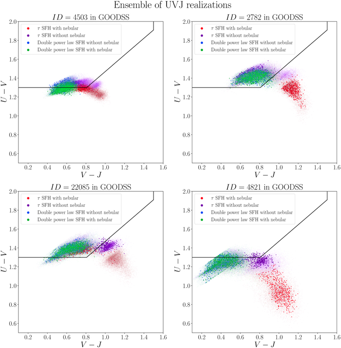
Figure 5. The UVJ plane for photometric resampling of the ensemble of individual galaxies (Monte Carlo simulated photometry). The posterior UVJ colors from the unperturbed photometry are shown with darker points, and the lighter points represent the posterior UVJ colors for the disturbed photometries on the UVJ color plane. This is a zoomed-in version of the UVJ plot showing the separation of different models. This figure shows how the change in the model assumptions (i.e., SFHs, including nebular emission) can change the UVJ color posterior distribution, which can affect our selection based on the UVJ colors.
Download figure:
Standard image High-resolution image4.2. Uncertainty of Selection Based on Observed Colors
To find the effect of photometric uncertainties on the selection based on the observed colors, we generate 105 realizations for every galaxy and assign a likelihood based on the number of realizations that fall into the hard selection criteria to the total number of realizations. The results for the GOODS-South galaxies are shown in Figure 6, where they are colored and resized based on the assigned likelihood. Few candidates fall outside of the selection criteria, but when we include the photometric uncertainties, we find realizations that fall in the selected region. On the other hand, few galaxies fall inside the criteria, but because of their photometric uncertainties, they do not show a clear indication of being quiescent.
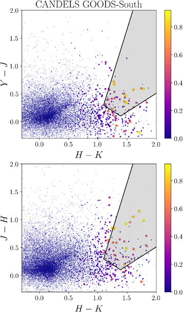
Figure 6. The figure shows the J − H vs. H − K and Y − J vs. H − K planes of CANDELS in the GOODS-South field. The larger and yellower data points show more chances of being quiescent given the photometry measurements and their uncertainties. Here we show just the effect of the photometric uncertainty.
Download figure:
Standard image High-resolution image4.3. Uncertainty of SED Fitting–based Selections
With having a posterior distribution of every physical parameter, we can estimate the uncertainties of these parameters. We use the resampling method mentioned above to get even more reliable error estimates (more details on the effect of the sampling error can be found in Higson et al. 2018).
Here we used the same sample from the SED fitting results for finding the sensitivity of the UVJ colors on photometric uncertainties. We follow the effect on the posterior ψSFR, which is the critical parameter in the SED-based selection discussed in Section 3.3. As Figure 7 shows, for most of the sample used, the τ-model SFH is more susceptible to photometric uncertainties than the double power law, which has more stable results under photometric perturbations similar to the UVJ colors. Also, including the models' nebular emission leads to models with UVJ colors that are further away from the quiescent region and hence reduce the number densities of the quiescent population.
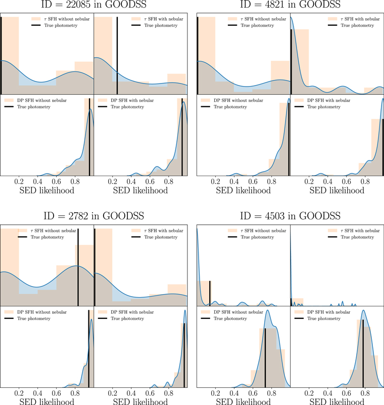
Figure 7. Here we show the dependence of the likelihood assigned in the SED selection on photometric uncertainties. The ψSFR likelihood for several galaxies and their bootstrapped photometries assumes Gaussian uncertainties. For each galaxy, the top left and right panels are the τ model without and with nebular emission, respectively, and the bottom left and right panels are the double power law without and with nebular emission, respectively. The histograms show bootstrapped sample photometries, and the curve is their simple kernel density estimate. The black line shows the quiescent likelihood from the SED from true photometry. The likelihood estimate from the τ models is shown to be more sensitive to possible variations under photometric uncertainties.
Download figure:
Standard image High-resolution imageIn this section, we found the effect of the photometric uncertainties on each method's assigned likelihood. As mentioned in Section 3.2, for finding the likelihood based on the observed colors for all of the galaxies in the CANDELS fields, we assign a likelihood to every photometric realization of a galaxy based on their proximity to the selection boundary, then we take the average of these as the observed color likelihood for that galaxy. By doing this, we can take into account both the photometric uncertainties and the closeness to the selection boundary. Since we only calculated the effect of the photometric uncertainties on likelihoods based on the UVJ- and SED-based selection for a subsample of galaxies, we did not incorporate the photometric uncertainties in the final assigned likelihood of these methods.
5. Number and Stellar Mass Densities
Using the final sample of massive and evolved galaxies, as presented in Table 5, we now estimate their number and mass density across the CANDELS fields. We divide the candidates based on their redshifts into two bins,  and
and  , approximately representing the same comoving volumes. To find the most reliable candidates, we need to assign a threshold for our likelihood. However, in order to follow this threshold's effect, we impose three different values on the final likelihoods. These thresholds are shown as error bars in Figure 9. The upper limits are for galaxies with an assigned likelihood of more than 0.3, the lower limits are for those with a likelihood of more than 0.7, and the measurement points are for those with a likelihood of more than 0.5. The variation caused by changing the selection threshold is larger than the typical Poisson noise. However, we take into account the Poisson noise as an independent source of uncertainty (Figure 8). We find the number/stellar mass densities after taking into account the incompleteness of our sample, as discussed in the next section.
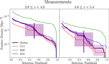
Figure 8. The comoving number densities for different selection methods and the median indicator used for the selection of the final sample are plotted. The shaded area around the median line shows the 1σ Poisson noise at a given threshold. We define the upper bound as the number density at a threshold of 0.3 and the lower bound as 0.7, including the Poisson noise. The error bars show the uncertainty as upper and lower bounds. The shaded rectangles correspond to variations in the number densities due to variation in the selection threshold ([0.3, 0.7]).
Download figure:
Standard image High-resolution image5.1. Completeness
To estimate the completeness of the sample used, we follow the prescription adopted in Pozzetti et al. (2010). We divide the CANDELS galaxies into the two redshift bins mentioned above. We find the 20% of the galaxies with the faintest apparent magnitude in the H band, with sSFRs lower than 75% of the galaxies in that redshift bin. We calculate the Mlim, defined as the mass that the galaxy would have if it were at the survey limiting magnitude (Hlim = 26; assuming a constant mass-to-light ratio); in other words, we find  . Then we define the fraction of the sample with
  as the completeness of the quiescent galaxies with that mass range. The effective volume of the survey at each redshift bin is defined to be Veff = Vco η(z), where Vco is the comoving volume at each redshift bin and η(z) is the completeness of the sample for
  at each redshift bin of the quiescent population.
5.2. Comparison to Model Predictions
In this section, we find the target population predicted from the several existing models listed below and compare their number and stellar mass densities with the sample found in this study.
- 1.Simulated infrared dusty extragalactic sky. We use the simulated catalog presented in Béthermin et al. (2017), which uses the abundance matching technique for occupying dark matter halos from the Bolshoi–Planck simulation (Klypin et al. 2016; Rodríguez-Puebla et al. 2016) and an updated version of the two star formation modes (2SFM) galaxy evolution model (Sargent et al. 2012; Béthermin et al. 2012) from which a light cone covering 2 deg2 was produced.
- 2.Universe machine. We employ the available CANDELS light cones produced by the universe machine semiempirical model, which uses the same Bolshoi–Planck simulation for halo properties and mass assembly histories. There are eight realizations for each field in CANDELS, and we use all of these realizations (Behroozi et al. 2019).
- 3.Eagle simulation. We use the Eagle cosmological hydrodynamical simulations of a box with L = 50 and 100 comoving megaparsecs (cMpc) on each side. We use RefL0050N0752, RefL0100N1504, and AGNdT9L0050N0752, in which the first two are the reference physical model used and the last one has a higher AGN heating temperature and lower subgrid black hole accretion disk viscosity. All of these simulations have the same mass resolutions (Crain et al. 2015; Schaye et al. 2015; McAlpine et al. 2016; The EAGLE team 2017).
- 4.IllustrisTNG simulation. We use the latest IllustrisTNG cosmological hydrodynamical simulations of a box with L = 100 and 300 cMpc on each side. There are three resolutions for each simulation box, and here we used the highest resolution (Marinacci et al. 2018; Naiman et al. 2018; Nelson et al. 2018, 2019; Pillepich et al. 2018; Springel et al. 2018).
To identify the quiescent galaxies in the simulations and be consistent with the observation of the massive evolved galaxies at z > 2, which have been known to be quite compact,  (Daddi et al. 2005; Trujillo et al. 2006; Trujillo et al. 2007; van Dokkum et al. 2008; Newman et al. 2010; Damjanov et al. 2011; van der Wel et al. 2014), we use the stellar mass and SFRs within twice the half-mass radius. Donnari et al. (2019) showed that the star formation main sequence in the IllustrisTNG100 for z > 2 is quite identical when assuming physical properties within an aperture of 5 kpc compare to the twice the half-mass radius definition for SFR measurements averaged over 10 and 1000 Myr. Also, following Merlin et al. (2019) and staying consistent in our comparison within the simulations, and since the physical properties of the Eagle simulations are available within certain apertures in the range 1–100 kpc, we use the physical properties within an aperture that is closest to four times the half-mass radius. For all of the models, we select galaxies with stellar masses
  and sSFRs within the half-mass radius lower than the evolving sSFR constraint employed in Pacifici et al. (2016), as sSFRlim = 0.2/tU(z), where tU(z) in Gyr is the age of the universe at redshift z. Carnall et al. (2019a) showed this to be consistent with the ψSFR measure used in this work across different redshifts.
Figure 9 shows the comparison between the observed number density of the quiescent galaxies within the corresponding comoving volumes, corrected for their completeness. The observed and predicted counts from the numerical simulations and empirical models of galaxy evolution are in generally good agreement. However, at the higher end of the redshift distribution, there are more observed candidates than predicted by models by a factor of ∼5. Nevertheless, it is somewhat consistent with the uncertainties shown in Figure 9 (especially in the case of the universe machine). Additionally, the presence of possible contaminants in the sample can ameliorate the tension.
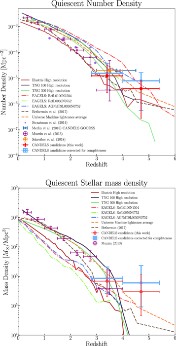
Figure 9. The comoving number and stellar mass density of the massive quiescent galaxies (defined as those with  and sSFR ≤ 0.2/tH(z) Gyr−1, in which tH is the age of the universe at redshift z) in two redshift bins from this work are overplotted as red data points on those from IllustrisTNG, and EAGLE simulations for different volumes are shown. The average of the universe machine (Behroozi et al. 2019) for all of the CANDELS's light-cone realizations is the orange dashed line. The model from Béthermin et al. (2017) is shown with the brown dashed line. Measurements from Muzzin et al. (2013), Straatman et al. (2014), Schreiber et al. (2018), and Merlin et al. (2018) are shown as purple, violet (number density data points without error bars) orange, and blue data points, respectively. The error bars show a 1σ uncertainty in the measurements, except for the error bars of this work, which are upper and lower limits of the measurements, taking into account the dependence of the measurement on artificial selection thresholds and the 1σ Poisson uncertainty.
Download figure:
Standard image High-resolution imageFigure 9 further shows the stellar mass density for our sample compared to the simulations and empirical models. We used the mass catalog from CANDELS to measure the stellar mass density. The tension between the stellar mass density for our sample and the simulations seems to be worse; however, the argument above for the number density applies here as well. The stellar mass measurements from the SED fitting results when including nebular line emission can also mitigate the tension, as the presence of the nebular lines can reduce the contribution from the continuum part of the SED, which can result in lower inferred stellar masses. Also, looking at the mass distribution of the selected samples from models and our CANDELS candidates (Figure 10) shows that the CANDELS candidates are relatively more massive than their counterparts in models, except for those from the TNG simulations. The TNG100-1 sample is shown to be more massive, and, using the fact that the stellar mass density at the highest redshift bins is lower than what we found here, we argue that the sample galaxies from the TNG tend to build their stellar mass later and at a higher rate than what is suggested from the CANDELS sample, similar to what Fontana et al. (2009) found. Also, by looking at the merger tree information of the selected sample (Rodriguez-Gomez et al. 2015) and following their history back to their formation epoch, we find the mass assembly and SFHs of the selected sample to check whether it is consistent with their selection as quiescent galaxies. Figure 11 shows the median and 20th and 80th percentiles of the mass assembly and SFR history of the sample selected. The SFHs were calculated from two SFR measures, one within the half-mass radius and one within twice the half-mass radius. Figure 11 reveals that the TNG sample at the lowest redshift bin is consistent with quenching even within twice the half-mass radius. Although the higher-redshift sample shows modest evidence of quenching within the half-mass radius, the star formation seems to continue outside of the half-mass radius.
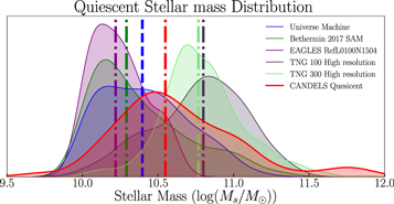
Figure 10. Stellar mass distribution of the candidates found here compared with semianalytical models and hydrodynamical simulations. The y-axis shows the kernel density estimate of the relative frequency (using a Gaussian kernel and Scott's rule for bandwidth selection).
Download figure:
Standard image High-resolution image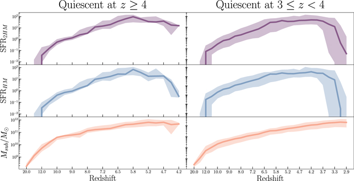
Figure 11. History of total subhalo mass assembly and SFR within the half-mass radius (SFRHM) and twice the half-mass radius (SFR2HM) from the IllustrisTNG100-1 simulation merger trees and following the most massive progenitor branch for the selected sample of quiescent galaxies based on the stellar mass and SFR measurements defined within the half-mass radius. The solid lines show the median history, with the shaded area corresponding to the 20th and 80th percentiles. As the figure shows, the higher redshift bin candidates show that the SFR within the half-mass radius is decreasing more rapidly than the star formation within twice the half-mass radius as they evolve.
Download figure:
Standard image High-resolution image
6. Discussion and Conclusion
In this study, we used three methods of selecting quiescent galaxies at high redshift. Using the grading scheme explained in Section 3, we minimized the effect of selection criteria by assigning a likelihood measure to each galaxy under each selection method. Figure 8 shows the number density measurements from different methods, the composite indicator (median) we used in the final selection, and their dependence on the selection thresholds. We also investigated the effect of the photometric uncertainties to understand the degree to which the result represented here could be affected. We combined these likelihoods by taking the median across different methods. The results from this study are consistent with similar investigations in CANDELS fields. Nayyeri et al. (2014) found 16 candidates in GOODS-South, of which seven are the same as what we found as candidates. Also, Merlin et al. (2019) found 102 candidates across all of CANDELS, with 36 being the same as those found here. More than half of the proposed candidates that are missing from our sample but reported in Merlin et al. (2019) showed more substantial Bayesian evidence when they were fitted with a τ SFH and a double power-law SFH compared to the constant SFHs employed in Merlin et al. (2019). This indicates that the selection is sensitive to the form of the SFH assumed.
We do not expect a significant difference between the two methods, since UVJ colors are expected to follow the sSFR of the model galaxies. However, they react differently to somewhat arbitrary criteria on either the UVJ plane or the sSFR. Moreover, we showed the classification based on the UVJ colors and SEDs to be strongly dependent on the choice of the SFH and, in the case of the τ model library, particularly susceptible to photometric uncertainties.
We found no strong evidence in favor of any SFH, similar to what found in Carnall et al. (2019a). However, the double power law showed more substantial evidence with less sensitivity to photometric uncertainties. Also, models that included nebular emissions showed stronger evidence. However, in the grading scheme defined here, we weighted each galaxy's likelihood by its respective evidence so that different models contribute to the likelihoods based on their relative Bayesian evidence.
The selection based on observed colors only uses a few passbands and does not require a search through the parameter space to find the best-fit model. Therefore, it is computationally more feasible than SED- or UVJ-based selections when a measure of the sensitivity to photometric uncertainties is needed. Hemmati et al. (2019) proposed a faster method of measuring the physical properties of galaxies and their uncertainties using Kohonen's self-organizing map (SOM; Kohonen 1982). The SOM is a neural network that maps the entire color space of galaxies into lower dimensions while preserving the topology of the input space (Kiviluoto 1996; Villmann et al. 1997). This feature ensures that we can have measurements with stable behavior under photometric uncertainties.
We find that the number and stellar mass densities of the candidates are generally consistent with the prediction of the numerical simulations. However, the agreement becomes less pronounced at higher redshifts, where numerical simulations underpredict the number/stellar mass densities of the quiescent galaxies.
Although the final sample purity requires spectroscopic observations, we employ a conservative approach for the completeness correction used in our number and stellar mass density measurements. In the sense that if we had used the model galaxies with a quiescent stellar population with Fsps (Conroy et al. 2009; Conroy & Gunn 2010),15 we get completeness levels that would make the number and mass densities even higher than what we showed here, especially at a higher redshift bin.
Using the number densities found here and an abundance matching technique, we predict an upper limit for the lowest halo masses of these galaxies and the corresponding lower limit for the highest efficiency of galaxy formation (Vale & Ostriker 2004; Wiklind et al. 2008; Conroy & Gunn 2010; Guo et al. 2010; Behroozi et al. 2010; Moster et al. 2010; Trujillo-Gomez et al. 2011; Moster et al. 2013; Reddick et al. 2013). Here we use the abundance matching technique described in Behroozi et al. (2013a), which matches galaxies in the order of decreasing stellar mass to the decreasing peak historical halo mass, according to their accretion history. Therefore, we find the peak historical halo mass corresponding to the number density of candidates using the cumulative peak historical mass function from Behroozi et al. (2013c) at a given redshift. We find the corresponding dark matter halos of mass Mh ≈ 4.2, 1.9, and 1.3 × 10¹² M⊙ at different redshift bins in Table 6 centered at z = 3.4, 4.1, and 4.7 and Mh ≈ 6.5, 4.7, and 4.5 × 10¹² M⊙ for the lower bound of the number densities, respectively. The estimated halo masses are similar to the critical shock-heating halo mass at these redshifts (Birnboim & Dekel 2003; Kereš et al. 2005; Cattaneo et al. 2006), at which the transition from cold-mode accretion into partly hot-mode accretion happens (Dekel et al. 2009). This transition could explain part of the quenching mechanism simply by shutting off the accretion of most of the cold gas into the halo. Although the fraction of cold-/hot-mode accretion is higher than in the halos of the same size at a lower redshift, the halo masses found here suggest a relatively lower fraction of cold-/hot-mode accretion than the less massive halos at the same epoch.
This agrees with the "cosmological starvation" scenario as a quenching mechanism, which suggests that there is a tight correlation between the SFRs and the mass accretion rate onto the halo (e.g., Larson et al. 1980; Balogh et al. 2000; Van Den Bosch et al. 2008) and was shown to be able to explain the relatively quick quenching time for massive central galaxies at high redshift (Argo simulations; Feldmann & Mayer 2015). The relatively high SFR required for building the stellar mass within a short timescale is consistent with submillimeter galaxies that exhibit a high SFR of order of a few hundred M⊙ (e.g., Marchesini et al. 2010; Swinbank et al. 2013) as a potential progenitor of these poststarburst systems (e.g., Toft et al. 2014; Wild et al. 2016; Wild et al. 2020).
Table 6. The Number Density Measurements and Calculated Upper and Lower Bounds (before Completeness Correction) Used in Figures 9 and 8
| Redshift Bin | Completeness | Number Density (Mpc−3) | Upper Bound (Mpc−3) | Lower Bound (Mpc−3) |
|---|---|---|---|---|

|
0.8 | 1.2 × 10⁻⁵ | 3.1 × 10⁻⁵ | 2.8 × 10⁻⁶ |
| 4.0 ≤ z < 5.4 | 0.5 | 4.1 × 10⁻⁶ | 8.2 × 10⁻⁶ | 2.7 × 10⁻⁷ |
| 2.8 ≤ z < 5.4 | 0.7 | 8.1 × 10⁻⁶ | 1.9 × 10⁻⁵ | 1.7 × 10⁻⁶ |
Note. Lower and upper bounds correspond to the selection thresholds of 0.7 and 0.3, respectively. Poisson errors are included in the bounds.
Download table as: ASCIITypeset image
Therefore, we suspect that a part of the quenching scenario of these systems could be that there was a phase of high accretion of gas into halos, which leads to high levels of SFRs and the subsequent mass buildup. Then the accretion of cold gas declines as the starvation phase begins, possibly by transiting to hot-mode accretion of the gas into the halo, followed by an "overconsumption" phase (McGee et al. 2014; Balogh et al. 2016), in which massive galaxies at high redshift use their gas in a depletion timescale that leads to their relatively fast quenching (in ∼a few hundred Myr). Similarly, Estrada-Carpenter et al. (2019) found that massive galaxies at  enriched quite rapidly to approximately solar metallicities as early as z ∼ 3. However, radio mode AGN feedback may still be required for keeping the galaxy quiescent and suppressing any residual star formation by driving out the remaining gas, as well as possible later accretion of a cold gas stream that penetrated the hot halo, in combination with stellar feedback and gravitational heating (Best et al. 2005; Bower et al. 2006; Croton et al. 2006; Feldmann & Mayer 2015; Man et al. 2019; Falkendal et al. 2019).
Similar to what has been observed at lower redshift, we find the quiescent sample found here to be consistent with the green valley (quenching) transition stellar mass (log(Ms/M⊙) ∼ 10.7) going all the way out to z ∼ 5. This points to the importance of this stellar mass scale in the quenching of the galaxies even at higher redshifts. We find that the number density measurements and their corresponding halo masses are consistent with halo quenching as the main mechanism (e.g., Rees & Ostriker 1977; Blumenthal et al. 1984; Kereš et al. 2005; Dekel et al. 2009). However, certain versions of the AGN quenching models can achieve the same number densities for quiescent galaxies (e.g., Chen et al. 2019).
Results suggesting that cosmological starvation plays a crucial role in the quenching of the massive quiescent galaxies at high redshifts are based on the abundance matching technique. However, this is based on the halo mass functions, which could underestimate the number of massive halos at high redshifts. The TNG simulation sample of quiescent galaxies and their progenitor history from their corresponding merger tree shows that the primary quenching mechanism is the quasar-mode energy injection by AGNs. These point to AGN activity as the primary quenching mechanism of the candidate galaxies. However, similar to what we found here, it is proposed that the "overconsumption" scenario is the primary driver of the environmental quenching for the massive quiescent galaxies at  (Chartab et al. 2020), with massive quiescent galaxies residing in overdense regions (more than 20% more quiescent in overdense regions), which shows that environment has a crucial role in the cosmological starvation scenario.
We acknowledge the Virgo Consortium for making their simulation data available. The EAGLE simulations were performed using the DiRAC-2 facility at Durham, managed by the ICC, and the PRACE facility Curie based in France at TGCC, CEA, Bruyèresle-Châtel.
Appendix: Selection Function
To quantify the effect of decision boundaries, we use an extended logistic function to differentiate between points closer to boundaries and those that reside well beyond the boundaries. A transformation takes the distance from the selection boundary and produces a value between zero and 1 in which the value closer to zero represents a galaxy that resides in the star-forming section and far from the selection boundaries and the value closer to 1 is the counterpart inside the quiescent region. However, any squashing function that takes a value from  and maps it to [0, 1] with the limiting behavior discussed above can do the job. We use a generalized logistic function,

in which A, K, B, C, Q, and M are free parameters. However, we can fix several of them without losing the needed features and by the fact that we are interested in maps from  to [0, 1]. Changing the parameters of this function can change the values we use to distinguish between different candidates. However, the utility of this method is to compare different candidates given a set of chosen selection parameters, and we do not care about a particular value. We are interested in whether a given candidate is more likely to be quiescent than other candidates. A "reasonable" choice of these parameters (Table 7) only generalizes the selection methods without losing information compared to applying a hard selection function.
Table 7. Choice of Criteria for the Selection Functions
| Selection | Criteria | Source | Set | Likelihood Function | Final Criteria |
|---|---|---|---|---|---|
| x1 = 3.44 − (Y − J) − 3.40 × (H − K) | A1 | μ1(x1) | |||
| x2 = − 1.03 + (Y − J) + 0.67 × (H − K) | A2 | μ1(x2) | |||
| x3 = 0.83 + (Y − J) − 0.67 × (H − K) | A3 | μ1(x3) |

|
||
| Observed colors | x4 = 2.48 + (J − H) − 2.80 × (H − K) | Nayyeri et al. (2014) | A4 | μ1(x4) | ∪ |
| x5 = − 1.70 + (J − H) + (H − K) | A5 | μ1(x5) |

|
||
| x6 = 0.16 + (J − H) − 0.43 × (H − K) | A6 | μ1(x6) | ∩ | ||
| x7 = S/N(U) − 2 | A7 | μ2(x7) |

|
||
| x8 = S/N(B) − 2 | A8 | μ2(x8) | |||
| y1 = (U − V) − 0.88 × (V − J) − 0.59 | B1 | μ1(y1) | |||
| y2 = (U − V) − 1.2 | Whitaker et al. (2012) | B2 | μ1(y2) | ||
| y3 = 1.4 − (V − J) | B3 | μ1(y3) |

|
||
| y4 = S/N(J) − 2 | B4 | μ2(y4) | ∪ | ||
| UVJ | y1 = (U − V) − 0.88 × (V − J) − 0.59 | C1 | μ1(y1) |

|
|
| y2 = (U − V) − 1.3 | Muzzin et al. (2013) | C2 | μ1(y2) | ∪ | |
| y3 = 1.5 − (V − J) | C3 | μ1(y3) |

|
||
| y1 = (U − V) − 0.88 × (V − J) − 0.56 | D1 | μ1(y1) | ∩ | ||
|
Straatman et al. (2014) | D2 | μ1(y2) | B4 | |
| y3 = 1.6 − (V − J) | D3 | μ1(y3) | |||
| Likelihood Functions | Logistic Parameters |
|---|---|
| μ1 | A : 0, K : 1, C : 1, Q : 3, B : 20, M: 2 |
| μ2 | A : 1, K : 0, C : 1, Q : 50, B : 1.4, M: 0.25 |
Note. Sets A and B are defined {(u, μ(u))∣u∈U}, in which A is the selected fuzzy set and U is the set of all galaxies. The logistic parameters chosen for each likelihood function are specified.
Download table as: ASCIITypeset image
To combine different criteria consistently, we assume that the function Y(xi) is the membership likelihood of the ith galaxy in the fuzzy set defined for specific criteria (Y is a form of membership function (μ)),

in which U is the set of all galaxies, and μA is the membership likelihood of the galaxies in criterion A. Also, for combining different criteria, we use the following rules for t-norm (intersection) and t-conorm (union):
Footnotes
- 14
- 15
Using τ model SFHs with τ = 0.2 Gyr and an age equal to the age of the universe at each redshift bin with solar metallicities.