


Abstract
In this work, we analyze the long-term cosmic-ray modulation observed by the Hermanus neutron monitor, which is the detector with the longest cosmic-ray record, from 1957 July. For our study we use the force-field approximation to the cosmic-ray transport equation, and the newest results on the mean free paths from the scattering theory. We compare the modulation parameter (ϕ) with different rigidity (P) dependences: P, P2, and P2/3. We correlate them with solar and interplanetary parameters. We found that (1) these rigidity dependences properly describe the modulation, (2) long-term cosmic-ray variations are better correlated with the magnitude of the heliospheric magnetic field (HMF) than the sunspot number, solar wind speed, and tilt angle of the HMF, and (3) the theoretical dependence of the parallel mean free path on the magnetic field variance is in agreement with the modulation parameter and therefore with the neutron monitor record. We also found that the force-field approximation is not able to take into account the effects of three-dimensional particle transport, showing a poor correlation with the perpendicular mean free path.
Export citation and abstract BibTeX RIS
1. Introduction
Variations in the cosmic-ray intensity have been observed on a continuous basis since 1936, with sporadic measurements since 1932. The Carnegie Institute of Washington sponsored the development of a "precision recording cosmic-ray meter" (Compton et al. 1934), of which five were installed in the USA, Mexico, Peru, New Zealand, and later on, in Greenland. Data from these instruments were distributed widely and provided the evidence that the cosmic-ray intensity in the 3–20 GeV range is under short-term (monthly) and long-term (11 yr) solar control (Forbush 1954). John Simpson (Simpson 2000) introduced the neutron monitor (NM) in 1951, and by the time of the International Geophysical Year (IGY) in 1957, more than 50 NMs were installed worldwide. Larger "super-NMs" replaced the original ones in the 1960s (Carmichael 1968), and a worldwide network of over 40 instruments is currently in operation. Prior to 1936, there were a number of high-altitude well-calibrated ionization chamber measurements that extend our knowledge back to the 1933 sunspot minimum. As a consequence, we now have records with high time resolution of the cosmic-ray intensity at Earth for the past eight solar cycles, 1933–2019. These observations were augmented by satellite and spacecraft observations starting in 1965. Furthermore, as outlined below, measurements of the annual cosmogenic radionuclides 10Be and 14C from 1389 (McCracken & Beer 2015) demonstrate that the 11 yr modulation of the cosmic radiation has been present throughout the entire period.
Variations in cosmic-ray intensity are the consequence of deflection of the galactic cosmic rays by the time-varying solar magnetic field that is convected away from the Sun by the solar wind. Sunspots are the consequence of the diminution of the light that is emitted by the Sun by strong, localized magnetic fields, and they provide an independent record of the magnetic activity of the Sun.
The NM and satellite measurements made over the last 68 yr have revealed two basic properties:
- 1.The intensity at Earth varies with time. Figure 1 shows that this occurs in response to solar activity, as indicated by the sunspot number (SSN), with a fundamental period of ≈11 yr. All cosmic-ray detectors that are sensitive to particles with rigidity (energy per unit charge) <20 GV observe this variation. The amplitude of the variation increases with decreasing rigidity.
- 2.The Voyager and Ulysses space missions away from the near-Earth environment have measured the spatial variations in the intensity. The two Voyager spacecraft have shown that the intensity for the energy range below ≈500 MeV/n increases at a rate of ≈1%/au at solar minimum conditions, and ≈2%/au at solar maximum (Moraal 2013). Voyager 1 crossed the boundary of this modulating region on 2012 August 25 at a distance of ≈122 au (Stone et al. 2013; Burlaga & Ness 2014) to observe the unmodulated interstellar intensity. The Ulysses spacecraft observed the inner heliosphere (radial distance <5 au) at high northern and southern latitudes, to discover that there is a latitudinal gradient of a few percent per degree (e.g., Heber et al. 2008), much smaller than was previously anticipated.
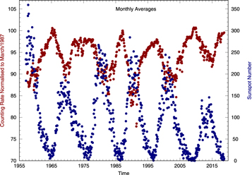
Figure 1. Monthly values of counting rate for the Hermanus NM (normalized to solar minimum conditions in 1987 March) and SSN.
Download figure:
Standard image High-resolution imageSunspots do not cause modulation. They are rather an indication of the time variation of other solar activity parameters such as the solar and heliospheric magnetic fields (HMFs), solar wind velocity, turbulence in the HMF, and episodic disturbances in the heliosphere caused by solar flares, coronal mass ejections, corotating interaction regions, merged interactions regions, and globally merged interaction regions (see, e.g., McDonald 1998, and references therein). These disturbances are listed in increasing time and spatial scale. The aim of cosmic-ray modulation studies is to determine quantitatively how these variables create the propagation conditions that explain the cosmic-ray modulation.
It is important to understand these time variations in detail during the technological era since about 1950, because it allows one to extrapolate solar and heliospheric conditions back into the past in two ways. First, solar activity has been observed for up to 400 yr in several parameters. Figure 2 is a summary of 20 of these parameters and of the period over which they have been observed. The SSN, of which a part is plotted in Figure 3, covers the longest period. It clearly shows the well-known 11 yr activity cycle and the differences from one cycle to the next. Over the past two decades, there has been much debate about different reconstructions of the SSN. There are mainly two sunspot records: the Wolf SSN, and the group SSN (see, e.g., Cliver & Herbst 2018). These two series differ from one another before ≈1885. However, in the past century, they are similar, except for the period of very high solar activity (see Figure 2 of Cliver & Herbst 2018). The use of different reconstructions will lead to different results. However, because our study covers about the last five decades of observations, we only use the Wolf SSN. We consider that the correlations of the force-field parameter with these two sunspot records will not differ from each other.
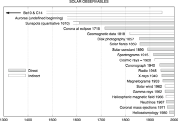
Figure 2. A summary of indicators of solar activity and the periods over which they have been measured. This figure is an update of the figure in Eddy (1976). After 1950 the atmospheric production of the cosmogenic radionuclides 10Be and 14C is heavily influenced by the anthropogenic radionuclides that were produced during the nuclear bomb tests (see, e.g., Muscheler et al. 2016).
Download figure:
Standard image High-resolution image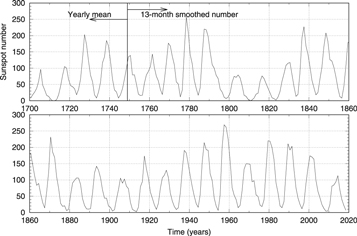
Figure 3. Yearly mean SSN up to 1749 and monthly 13-month smoothed SSN from 1749 up to the present (source: WDC-SILSO; Royal Observatory of Belgium, Brussels).
Download figure:
Standard image High-resolution imageSeveral solar minima have been even quieter than the minimum of 2009/2010, and it is generally accepted from indirect observations that during the Maunder Minimum of 1645–1710, solar activity almost ceased (see, e.g., Riley et al. 2015; Cliver & Herbst 2018, and references therein). These solar and heliospheric variations may therefore allow us to extrapolate the cosmic-ray intensity back for the last 400–500 yr. No systematic solar observations are available before that time.
The second way of extrapolation overcomes this limitation by analyzing the concentration of cosmogenic nuclides that were produced by cosmic-ray induced interactions in the atmosphere (see, e.g., Beer et al. 2012; McCracken & Beer 2015). The well-known 14C that is produced in this process is sequestered in biological material, while 10Be is preserved in polar ice as long as the ice accumulates with time. Time variations in the concentration of these nuclides are a direct indication of the time variation of the cosmic-ray intensity. Steinhilber et al. (2012) have summarized the work in this field during the past 30 yr, from which they inferred the cosmic-ray intensity during the last ≈10,000 yr. From this proxy for the cosmic-ray intensity, the authors deduced that solar activity has not been higher at any time during this period than in the current technological era. The 10Be record extends even farther back, up to 100,000 yr, but the statistical significance, time resolution, and absolute timing become progressively worse.
This second long-term extrapolation is unique. No other similarly measurable quantity older than about 500 yr is known. In view of our quest to understand climate change, it is also uniquely important. Climate changes are due to anthropological and natural causes. Some of the natural variations are in turn induced by solar activity. To disentangle the relative contributions of these two, it is therefore of crucial importance to understand the helioclimate as far back as possible.
This chain of backward extrapolation requires two fields of study. First, our ongoing cosmic-ray modulation studies attempt to describe the cosmic-ray variations due to solar and heliospheric variations in ever greater detail. Second, the quantitative relationship between cosmic rays and cosmogenic nuclides must be better verified, especially during the most recent 60 yr of the technological era. This requires studies of the atmospheric showers of secondary particles caused by cosmic rays, and the transport of these particles in atmospheric convection and dispersion before they settle as readily identifiable components such as 10Be in polar ice (see chapter 13 of Beer et al. 2012). This in turn requires a detailed understanding of the cosmic-ray atmospheric yield function, both experimentally (e.g., Caballero-Lopez & Moraal 2012) and by numerical simulation (Clem & Dorman 2000; Mishev et al. 2013).
This paper contributes to the first category of studies, i.e., to investigate to what extent we understand the long-term cosmic-ray intensity variations over the past four solar cycles in terms of variations of solar and heliospheric parameters.
In Section 2 we summarize the necessary cosmic-ray transport and modulation theory. The diffusion coefficients that appear in the equations depend on the scattering of the cosmic rays in the turbulent HMF. Therefore we consider in Section 3 what information can be gleaned from recent cosmic-ray scattering theories, and what conclusions can be drawn therefrom. Finally, in Section 4 we correlate the observed cosmic-ray modulation with SSN (from www.sidc.be/silso/datafiles and heliospheric parameters from the OMNIDATA (http://omniweb.gsfc.nasa.gov/). These parameters are combined in such a way that they produce our best theoretical estimate of the modulation.
We restrict the cosmic-ray observations to NMs. They alone provide a long-enough stable baseline that now stretches over more than five solar cycles.
2. Cosmic-ray Modulation Theory
The cosmic-ray transport equation for the evolution of the omnidirectional distribution function, f, with time, t, position vector,  , and momentum p is

where  is the solar wind velocity, and the diffusion tensor is given by

This tensor describes a diffusive flux  , where
  and κ⊤ are the diffusion coefficients parallel and perpendicular to the background magnetic field
  . The third term describes particle drift due to the wavy current sheet, as well as due to the gradient and curvature of the background magnetic field. The convective flux
  takes into account the Compton–Getting effect through the coefficient C. The last term of the equation describes adiabatic energy changes. The equation was first derived by Parker (1965), and the details of this and subsequent derivations and its various solutions were reviewed by Moraal (2013). The momentum variable may be changed to rigidity, P, or kinetic energy per nucleon, T, with
  , where A and Z are mass and charge numbers, respectively.
One of the frequently used solutions of the transport equation is the force-field formalism (see, e.g., Caballero-Lopez & Moraal 2004), which assumes steady state, spherical symmetry of the heliosphere, and ignores adiabatic energy changes. Thus, balancing the inward diffusive flux with the corrected outward convective flux, Equation (1) takes the following form:

When C = (1/3)∂lnf/∂lnP is introduced explicitly, the equation becomes a first-order partial differential equation,

with solution f(r, p) = constant = fb(rb, pb) along contours of the characteristic equation dp/dr = pV/(3κ) in (r, p) space. In this approximation the diffusion tensor Equation (2) is reduced to a single scalar coefficient κ. If this diffusion coefficient is separable in the form

the solution of Equation (4) is
where ϕ is called the force-field parameter. The modulation parameter ϕ is a convenient single parameter that describes the modulation as a function of the three variables solar wind speed, diffusion coefficient, and size of the heliosphere. It is important to note, however, that these three parameters cannot be deduced separately from cosmic-ray measurements at a single point in the heliosphere—only their integral effect is known, and therefore the solution contains a limited amount of physics.
The force-field solution is commonly used for rigidities P > 1 GV (in particularly for NM data analysis), with κ2 ∝ P and  . Then the solution of Equation (6) is

so that the force-field parameter ϕ has the physical meaning of a rigidity loss. Because rigidity has the dimensions of potential, it is often called the force-field potential. The assumptions as to the effective diffusion coefficient that make this interpretation possible are highly specific, and as such will form part of the discussion in the next section.
The omnidirectional distribution function, f, is related to the measured cosmic-ray intensity, jT, with respect to kinetic energy per nucleon, T, as jT = p2f. Thus, in terms of intensities, the force-field relationship f(r, P) = fb(rb, Pb) becomes

We apply this formalism to NM observations. These instruments do not measure the distribution function, f, or the related intensity or the particle density in a rigidity interval  , but rather the integral number of counts, N, above a minimum—or cutoff—rigidity, Pc. The relationship between the intensity of primary cosmic rays and the counting rate of an instrument inside the atmosphere is called the atmospheric yield function for that particular instrument. Mathematically, the process is described as follows: the counting rate N(Pc, x, t) of a detector at cutoff rigidity Pc, atmospheric depth x and time t is such that
where ji(P, t) is the spectrum of the primary species i above the atmosphere, and Si(P, x) is the atmospheric yield function due to this species.
Following the procedure described in Section 7 of Caballero-Lopez & Moraal (2012), we can obtain time variations in the force-field parameter from the counting rates that are registered in the NM stations. In particularly, we will compute Δϕ(t) = ϕ(t) − ϕ(1987), because this quantity does not depend on the choice of the interstellar cosmic-ray spectrum.
3. Mean Free Paths from Theory
Assuming that the force-field approach to the solution of the Parker (1965) cosmic-ray transport equation is valid, the connection between historic cosmic-ray intensities and the solar properties they encountered lies in the effective diffusion coefficient that is assumed in this approximation. Establishing such a connection, however, is no simple task. Many theories have been proposed to describe the scattering of cosmic rays in the heliosphere. The most likely candidates for this task, given their reasonable agreement with observations and numerical simulations of cosmic-ray diffusion coefficients, are the quasilinear theory (QLT) of Jokipii (1966), the weakly nonlinear theory (WNLT) of Shalchi et al. (2004b), and the nonlinear guiding center theory (NLGC; or one of its variants; see, e.g., Matthaeus et al. 2003; Shalchi 2006, 2009, 2010; Ruffolo et al. 2012). Shalchi (2009) provides in depth theoretical treatments of most the abovementioned theories. These scattering theories all require as a key input an expression for the power spectrum of the turbulent fluctuations of the HMF. These spectra depend upon basic turbulence quantities, such as the magnetic variance, and various correlation scales. Turbulence power spectra are discussed in detail by, e.g., Batchelor (1970) and Matthaeus et al. (2007), whereas more background on the abovementioned turbulence quantities can be found in, e.g., Matthaeus & Goldstein (1982), Petrosyan et al. (2010), Matthaeus & Velli (2011), and Bruno & Carbone (2013). These basic turbulence quantities have been observed to show a marked dependence on the solar cycle at Earth (see, e.g., Smith et al. 2006b; Burger et al. 2014; Zhao et al. 2018). It follows then that mean free paths derived from these scattering theories would be expected to depend on the solar cycle as well, and several studies have reported such a dependence. Chen & Bieber (1993) find from an analysis of cosmic-ray anisotropies and gradients as observed by means of NMs, that larger mean free paths are associated with solar minima, and smaller mean free paths with solar maxima. The authors also report a mean free path dependence on solar magnetic polarity. Nel (2016) and Zhao et al. (2018) both extensively analyze spacecraft observations, using the turbulence quantities so calculated as inputs for expressions for diffusion coefficients derived from the QLT and NLGC theories. Both authors report that the resulting mean free paths display solar cycle dependences.
The task of choosing which scattering theory to use is also not a simple one, as a decision has to be made as to what theory would yield realistic diffusion coefficients throughout the heliosphere based on observations and test particle simulations that are applicable to a limited number of turbulence scenarios (see, e.g., Giacalone & Jokipii 1999; Qin et al. 2002a, 2002b; Minnie et al. 2007a). On the other hand, observations of the high-energy parallel mean free path, as reported by, e.g., Palmer (1982), Bieber et al. (1994), and Dröge (2000), show significant variations in magnitude on an event-by-event basis, but display essentially the same rigidity dependences. At intermediate energies, these observations display the P1/3 rigidity dependence predicted by magnetostatic QLT, as opposed to the P0.6 rigidity dependence predicted by the WNLT (Shalchi 2009). Numerical simulations of the parallel mean free paths performed by Minnie et al. (2007a) show that WNLT yields results in better agreement with simulated parallel mean free paths than does QLT for a broad range of turbulence levels, with QLT providing reasonable agreement for the relatively low levels of turbulence (see also, e.g., Giacalone & Jokipii 1999) that are expected in the outer heliosphere (see, e.g., Zank et al. 1996; Smith et al. 2001). At high rigidities (above ∼1 GV), the WNLT and QLT results are essentially identical (Shalchi 2009), displaying a P2 rigidity dependence. As to the perpendicular mean free paths, the simulations performed by, e.g., Matthaeus et al. (2003) and Minnie et al. (2007a) show that the NLGC theory provides results in excellent agreement with simulations for a broad range of turbulence conditions, yielding also a relatively flat rigidity dependence that is in qualitative agreement with the observational findings of Palmer (1982). The perpendicular mean free path yielded by WNLT, on the other hand, does not provide results in as good agreement with simulations and observations (Minnie et al. 2007a). From the above, the NLGC theory (or one of the refining theories based on it, such as the extended NLGC (ENLGC) theory of Shalchi 2006) would appear to be the natural choice to make, and would appear to be the best candidate to describe an effective diffusion coefficient, given that the winding angle of the Parker field is very close to 90◦ in most of the heliosphere. This approach, however, requires as an input an expression for the parallel mean free path. This is usually based on results from QLT such as the parametrized expression of Zank et al. (1998) or the analytical work of Teufel & Schlickeiser (2003). The choice of QLT is motivated not only by the relatively reasonable agreement of this parallel mean free path with observations and simulations, but also by the availability of tractable analytical expressions for this quantity.
One such expression, employed in galactic cosmic-ray proton modulation studies by, e.g., Burger et al. (2008) and Engelbrecht & Burger (2013a), Moloto et al. (2018), and based on those derived by Teufel & Schlickeiser (2003) for a slab turbulence power spectrum that has a flat energy-containing range and an inertial range, is given by
where s denotes the spectral index (in absolute value) of the inertial range on the assumed slab turbulence power spectrum with 1 < s < 2 (Teufel & Schlickeiser 2003). This expression is the same as that employed by Nel (2016), and behaves similarly to the Zank et al. (1998) QLT result employed by Zhao et al. (2018). Note that Smith et al. (2006a) report from spacecraft observations a spectral index for the inertial range of −1.63 ± 0.14, although this is a matter of some debate (see, e.g., Forman et al. 2011; Li et al. 2011). The error bars on this value include both the Kolmogorov (1941) value of 5/3 and the Iroshnikov–Kraichnan value of 3/2 (Iroshnikov 1963; Kraichnan 1965). This distinction, however, would mostly affect the rigidity dependence of this mean free path at lower energies that are below those of relevance to this study. Furthermore, kmin = 1/λs the wavenumber corresponding to the turnover scale at which this inertial range commences,  the slab variance, B0 the background HMF magnitude (such as the Parker field), and R = RLkmin, RL being the (maximum) gyroradius. When we take the magnetic field dependence of the Larmor radius into account, this expression displays a B0s dependence for low rigidities, becoming independent of the HMF magnitude at high rigidities. Note that this dependence is only the explicit magnetic field dependence, and that the actual solar cycle dependence of λ∥ would differ due to the solar cycle dependences of the various turbulence quantities such as
  . At the highest energies relevant here, this expression therefore yields the expected P2 rigidity dependence.
Given the complexity of perpendicular mean free path expressions derived from the various scattering theories mentioned above (see, e.g., Shalchi et al. 2010; Engelbrecht & Burger 2013a; Qin & Zhang 2014; Engelbrecht & Burger 2015a, 2015b; Wiengarten et al. 2016), it is difficult to glean information as to their dependence on the HMF magnitude, for example. Shalchi et al. (2004a), however, derive tractable approximate analytical expressions for the perpendicular mean free path from NLGC, assuming a 2D turbulence power spectrum with a flat wavenumber dependence in the energy range, and some inertial range. This expression is also valid for the extended NLGC proposed by Shalchi (2006), and has been used in several modulation studies (Burger et al. 2008; Engelbrecht & Burger 2010; Sternal et al. 2011; Moloto et al. 2018). The expression presented by Burger et al. (2008) for a general ratio of slab to 2D variance is given by
with F2(ν) = 2πC(ν)F1(ν), F1(ν) = 2ν/(2ν − 1), 
![$[{\rm{\Gamma }}(\nu )/{\rm{\Gamma }}(\nu -1/2)]$](https://content.cld.iop.org/journals/0004-637X/883/1/73/revision1/apjab3c57ieqn13.gif) , and ν half the spectral index of the inertial range on the 2D turbulence power spectrum. The subscript "2D" refers to turbulence quantities associated with the 2D turbulence power spectrum, while ν denotes the spectral index of the inertial range on this spectrum. Both the perpendicular and parallel mean free paths discussed here are shown in Figure 4 as functions of rigidity at 1 au, using generic solar minimum turbulence quantity values as inputs, along with the Palmer (1982) consensus ranges. Note that if a turbulence transport model were used to model the basic turbulence inputs in these expressions, the rigidity dependences of these mean free paths would change in the outer heliosphere (see, e.g., Moloto et al. 2018). When we use Equation (10) as input, the perpendicular mean free path at high energies should then display a ∼P2/3 rigidity dependence, and at lower energies a ∼P1/9 dependence.
, and ν half the spectral index of the inertial range on the 2D turbulence power spectrum. The subscript "2D" refers to turbulence quantities associated with the 2D turbulence power spectrum, while ν denotes the spectral index of the inertial range on this spectrum. Both the perpendicular and parallel mean free paths discussed here are shown in Figure 4 as functions of rigidity at 1 au, using generic solar minimum turbulence quantity values as inputs, along with the Palmer (1982) consensus ranges. Note that if a turbulence transport model were used to model the basic turbulence inputs in these expressions, the rigidity dependences of these mean free paths would change in the outer heliosphere (see, e.g., Moloto et al. 2018). When we use Equation (10) as input, the perpendicular mean free path at high energies should then display a ∼P2/3 rigidity dependence, and at lower energies a ∼P1/9 dependence.
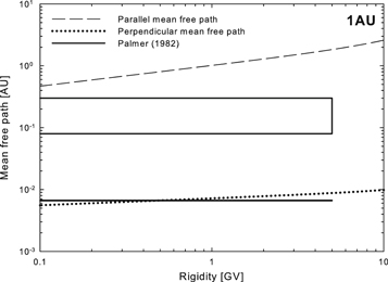
Figure 4. Proton QLT parallel and NLGC perpendicular mean free paths (Equations (10) and (11)) at 1 au as function of rigidity for parameters as discussed in Burger et al. (2008), along with Palmer (1982) consensus values.
Download figure:
Standard image High-resolution imageBoth Nel (2016) and Zhao et al. (2018) report that these parallel mean free paths are smaller during periods of high solar activity and larger during solar minima, with the opposite being true for the resulting perpendicular mean free paths. Zhao et al. (2018) also show that such solar cycle dependences would not be fully accounted for if only the solar cycle changes in the HMF were taken into consideration. These mean free paths also display complicated spatial dependences if turbulence quantities beyond 1 au, yielded by various turbulence transport models (see, e.g., Oughton et al. 2011; Usmanov et al. 2016; Wiengarten et al. 2016; Zank et al. 2017), taking into account observed latitudinal variations of turbulence quantities in the heliosphere (Forsyth et al. 1996; Bavassono et al. 2000a, 2000b; Erdös & Balogh 2005), were used as inputs for the turbulence quantities (e.g., Engelbrecht & Burger 2013a, 2015b; Chhiber et al. 2017; Moloto et al. 2018). Furthermore, mean free paths such as those discussed have, when used in conjunction with turbulence-reduced drift coefficients (see, e.g., Minnie et al. 2007b; Engelbrecht et al. 2017) in 3D stochastic modulation codes, led to computed galactic intensities in reasonable agreement with spacecraft observations at Earth (see, e.g., Engelbrecht & Burger 2013a, 2013b; Qin & Shen 2017) and even for several different solar minima (Moloto et al. 2018). The necessity of taking cosmic-ray drift effects into account, combined with the complicated spatial dependences and the fact that none of the diffusion coefficients described above display a P1 rigidity dependence, implies that a convection–diffusion or force-field approach would not be ideal to describe long-term modulation, and that the assumptions implicit to the effective diffusion coefficient used in these formulations are unrealistic. This latter point would call into question any conclusions drawn as to historic solar parameters from quantities such as the modulation potential.
The aim of this paper is to study the long-term cosmic-ray modulation at Earth, associated with variations in solar parameters. Therefore, we need to consider time and energy dependences of the mean free paths at 1 au. When we assume a Parker field, the magnetic turbulence is purely contained in its N-component (BN, north–south component). According to the analysis in Moloto et al. (2018) and assuming that λs and λ2D display little to no solar cycle dependences (see, e.g., Wicks et al. 2010; Zhao et al. 2018), it follows from Equations (10) and (11) that for low-rigidity cosmic rays, P ≲ 1 GV,

For high-rigidity cosmic rays, P ≳ 1 GV, however,

We should consider Equation (13) when we analyze NM observations. Moreover, we must use the rigidity dependence in λ⊥ in the case of the force-field approximation because the radial mean free path is expected to be dominated by this quantity as a result of the HMF geometry. We note that Equation (5) with diffusion coefficient κ in a separable form is in agreement with the mean free path expressions of Equations (12) and (13) that are obtained from turbulence analysis.
Recently, Burger & Engelbrecht (2018) analyzed the solar dependence of the correlation scale for the N-component of the magnetic field. They found that there appears to be a correlation between correlation length and magnetic variance, as proposed by Matthaeus et al. (1986). When we assume that these quantities would have the same time dependence, the parallel and perpendicular mean free paths for high-energy cosmic rays have the following dependence:

Zhao et al. (2018) analyzed the influence of the solar cycle on turbulence properties, and subsequently also on cosmic-ray diffusion coefficients, using a parallel mean free path similar to Equation (10), and a perpendicular mean free path expression identical to Equation (11). They showed the results for low-rigidity particles (≈0.445 GV). Our Equation (12), as can be seen in panel (B) in Figure 8, behaves in a manner that is in agreement with their mean free path calculations. At these lower energies, the parallel mean free path will be larger at solar minimum than at solar maximum, while the perpendicular mean free path shows very little in the way of a solar cycle dependence. For high energies (panel (C) in Figure 8), Equation (13) shows that parallel mean free path will also be larger during solar minimum than during solar maximum. The perpendicular mean free path shows a minor solar cycle dependence in that it is slightly larger at solar minimum than at solar maximum, but this is again not as clear as the dependence of λ∥. It is the extent of the solar cycle changes that now differs at high energies, and is expected to be larger than that reported by Zhao et al. (2018). Zhao et al. (2018) do not consider the effects on the various mean free paths of a correlation scale that depends on solar cycle because they do not find such a dependence in their analysis of the data, which is different to that employed by Burger & Engelbrecht (2018). An in depth analysis of these differences is beyond the scope of this study, but both possibilities are considered in that which is to follow. If both slab and 2D correlation scales display the same solar cycle dependence as the variance, the high-energy parallel mean free path will still be larger during solar maximum than during solar minimum, but the corresponding perpendicular mean free path would be approximately constant. For the sake of argument, however, if it were assumed that the 2D correlation scale displays a solar cycle dependence but that the slab correlation scale for some reason does not, then

In this case, the parallel mean free path would behave as in Equation (13), but the perpendicular mean free path should display a clearer solar cycle dependence, assuming greater values during solar maximum than during solar minimum. In the next section we present the implications of employing these assumptions as to turbulence properties as inputs for the effective diffusion coefficient for the NM observations of high-energy cosmic rays.
4. Analysis, Results, and Discussion
In this section we analyze the long-term modulation based on the Hermanus NM observations and solar activity parameters registered at Earth. It is a challenging task to maintain the calibration of a NM over many decades. Aging of the proportional counters; changes in the distribution of mass nearby; changes in the geomagnetic field; and electronic drifts, to name just a few, are all potential sources of one percent and greater long-term changes in counting rate. There is a worldwide network of more than 40 NM, and there have been several careful intercomparisons of data from a number of them. We have used the comparisons of Moraal & Stoker (2010) and Oh et al. (2013) to estimate that the long-term errors in the Hermanus data are ∼1%. Table 1 summarizes the intervals used in this work, along with data sources.
Table 1. Data Used in This Work
| Data | Time Interval | Source |
|---|---|---|
| Hermanus NM | 07/1957–10/2018 | http://natural-sciences.nwu.ac.za/neutron-monitor-data |
| OMNIDATA | 07/1966–09/2018 | http://omniweb.gsfc.nasa.gov/ |
| SSN | 07/1957–10/2018 | www.sidc.be/silso/datafiles |
| tilt angle HMF | 05/1976–10/2018 | http://wso.stanford.edu/Tilts.html |
Note. OMNIDATA parameters: HMF component (BR, BT, BN), magnetic field magnitude (B), and solar wind speed (V).
Download table as: ASCIITypeset image
4.1. Data: Time Variations
In Figure 5 we present the monthly averages and 12-month moving averages of the Hermanus counting rate (A), SSN (B), magnitude of the magnetic field (C), solar wind speed (D), and tilt angle of the HMF (E) from 1963 to the end of 2018. Blue (red) shadow bands indicate a two-year interval around solar maximum (minimum) in concordance with SSN. In general, these parameters follow the solar cycle dependence. However, some differences are clear. First of all, the NM counting rate in panel (A) reaches its maximum intensity a few months after the SSN minimum, which should be an indication that the cosmic rays observed at Earth are the result of the overall modulation in the entire heliosphere. Second, the magnitude of the magnetic field (C) shows higher values at solar maximum than at solar minimum, but this relation has no strong correlation. For the solar wind speed at Earth (panel (D)), the solar cycle dependence is not clear, as it is when we analyze its heliolatitude profile (reference of Ulysses). The tilt angle of the HMF presents a very well-defined solar cycle dependence.
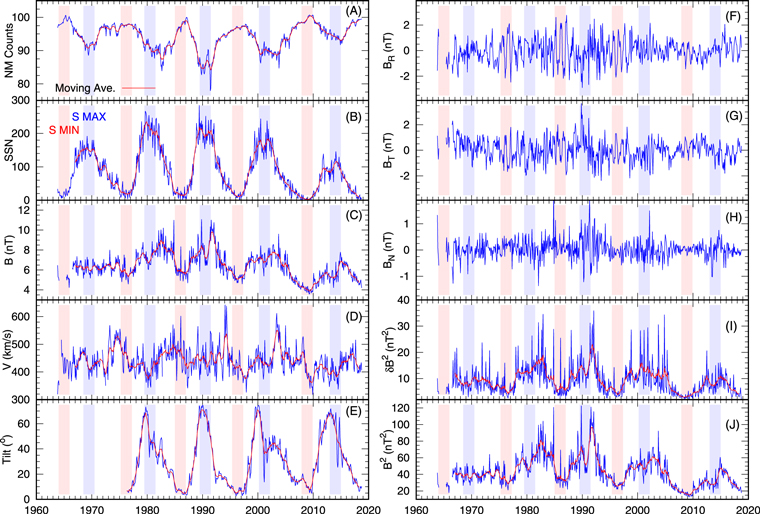
Figure 5. Monthly averages (in blue) and 12-month moving averages (in red) of the Hermanus counting rate (panel (A): normalized to 100% in 1987 March), SSN (panel (B)), magnitude of the magnetic field (panel (C)), solar wind speed (panel (D)), tilt angle of the HMF (panel E), radial component of the magnetic field (BR, panel (F)), azimuthal component (BT, panel (G)), north–south component (BN, panel (H)), variance of B, (δB2, panel (I)), and square of B (panel (J)).
Download figure:
Standard image High-resolution imageThe other parameters that we look at are the magnetic field components and their fluctuations. These are shown in the right panels of Figure 5. These B components do not show a clear solar cycle dependence, except for the variance of the BN component in panel (I) and the square of B in panel (J). This is important because these two quantities will probably influence the cosmic-ray transport through Equations (13) and (14) when long-term modulation is studied. We analyze this in detail in Section 4.4.
4.2. Correlation: NM Counting Rate and Force-field Modulation Parameter
Force-field approximation and scattering results presented in the previous section are used to analyze Hermanus observations. Then we compare our modulation results to the temporal variations of several solar parameters to explain the long-term cosmic-ray variations observed at Earth. We also investigate the role of using different rigidity dependences of the mean free paths in order to validate the force-field approximation for these studies.
The ultimate aim of the paper is to compare these experimental values of the modulation depth calculated from the Equation (6) using the measured values of V from the OMNIDATA, with values of κ (B, δB) as calculated from the scattering theory in Section 3.
We start our analysis with the calculation of the force-field parameter. More precisely, we analyze the variations in this parameter with respect to the modulation level in March 1987. This is because (1) the Hermanus NM counting rate is normalized to that time, and (2) the variations in ϕ do not depend on the interstellar spectrum. For this, we define δϕ(t) = ϕ(t) − ϕ(03/87). The modulation potential ϕ(03/87) is ≈0.407 GV (Caballero-Lopez & Moraal 2004).
As we mentioned before, the analysis of the force-field model is frequently based on the assumption that the diffusion coefficient is proportional to rigidity. In this case, ϕ has the units of GV. For comparison, we compute three cases: (1) the diffusion coefficient (and therefore the mean free path) ∝P, (2) ∝P2/3, and (3) ∝P2. The last two cases are related to the mean free paths in the high-energy regime in Equation (13). These cases lead us to three modulation parameters: δϕ1, in units of GV, δϕ2/3, in units of GV2/3 and δϕ2 in units of GV2.
Many previous works compute the force-field modulation potential (see, e.g., Usoskin et al. 2011, 2017; Ghelfi et al. 2017). These studies have shown that the estimation of this parameter differs depending on the local interstellar spectrum or the energy range that is used to infer it. Recently, Gieseler et al. (2017) proposed a modified force-field modulation potential based on two solar modulation parameters. However, in the NM energy range, their ϕ is equal to the value reported by Usoskin et al. (2011), which is in agreement with the δϕ1 we used here (e.g., Santiago et al. 2018).
We follow the procedure explained in Section 7 of Caballero-Lopez & Moraal (2012). This means that choosing a rigidity dependence of κ2, we solve the left-hand part of Equation (6) and obtain the value of δϕ that reproduces the counting rate according to Equation (9). The results are shown in Figure 6. We see that in all three cases, as expected, δϕ is correlated with the NM counting rate. Moreover, they have very similar time variations. This is because each of them is calculated to fit the rate. These plots may suggest that from the point of view of the force-field model, all three diffusion coefficient dependences on rigidity can be used to reproduce the NM observations. It is also important to note that in Figures 5 and 6 the (unsmoothed) monthly values of δϕ are always smoother that the variations in each of the individual parameters. This clearly reflects the integral nature of the modulation as a function of space and time.
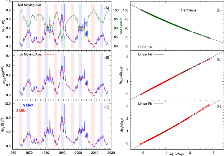
Figure 6. Left panels: monthly averages (in blue) and 12-month moving averages of the Hermanus counting rate (panel (A), right vertical axe), the force-field modulation parameter for diffusion coefficient proportional to rigidity, P (panel (A), or the force-field potential), to P2/3 (panel (B)), and to P2 (panel (C)). Right panels: correlations between the normalized force-field potential δϕ1 and the Hermanus counting rate (panel (D)), the force-field modulation parameter δϕ2/3 (panel (E)), and the force-field modulation parameter δϕ2 (panel (F)). The black line shows the least-squares fit. See text for an explanation.
Download figure:
Standard image High-resolution imageTo quantify the relationship between different parameters, we apply a least-squares fit procedure to their 12-month moving averages. First, we must note that our approximation, to ignore the temporal change term ∂f/∂t in Equation (1), is valid when we use the 12-month sliding averages in our correlations. At 400 km s−1 the solar wind and its embedded magnetic fields propagate out to 100 au in about 430 days, and this is therefore the duration of the "memory" of the system. Beyond this timescale, the temporal effects are lost. However, because of its simplicity, the force-field modulation model has been extensively used to analyze long-term cosmic-ray variations, particularly for studies of high-energy galactic cosmic-ray transport (in the NM energy range) where this approximation is more suitable (see, e.g., Caballero-Lopez & Moraal 2004, and reference therein).
Because the force-field modulation potential δϕ1 is the most commonly used parameter for analyzing the long-term modulation, we correlated all other parameters to this potential. For simplicity, we normalized the modulation parameter to its average value, so all quantities are dimensionless. In the analysis of the counting rate and δϕ1, we assume the relation reported by Usoskin et al. (2017) and Santiago et al. (2018), written here as

where a is the coefficient that must be calculated from the least-squares fit analysis. It is clear that N increases when δϕ1 decreases, and the counting rate decreases when δϕ1 increases. At the same time, this expression gives a counting rate of 100% for δϕ1 = 0, which is the normalization value in March 1987.
For other parameters, we use a linear least-squares fit, with an expression of the form, f(x) = ax + b. Here the independent variable is δϕ1. In Figure 6 (right panels) we plot the correlation between these parameters. The correlation coefficient and the least-squares fit are listed in Table 2. As we see, the correlations are very high, indicating that all three force-field parameters are a good proxy of the NM counting rate. This is not a surprise if we think that for a given time, each of these three parameters must represent the observed modulation depth (N(t)). This very strong relationship between the three force-field modulation parameters allows us to use only δϕ1 as a proxy for the cosmic-ray modulation.
Table 2.
Correlation Coefficient and Least-squares Fit for the Hermanus Counting Rate and the Force-field Modulation Parameters δϕ2/ and δϕ2/3/
 with Respect to the Normalized Force-field Modulation Potential (δϕ1/
 )
)
| Parameter | a | b | Correlation | Variance of |
|---|---|---|---|---|
| Coefficient | Residuals | |||
| Counts | (63714 ± 9)×10−6 | ⋯ | −0.9989 | 4.4 × 10⁻⁴ |
δϕ2/
|
1.070 ± 0.002 | −0.070 ± 0.003 | 0.9988 | 1.2 × 10⁻³ |
δϕ2/3/
|
0.9838 ± 0.0005 | 0.0163 ± 0.0006 | 0.9999 | 6 × 10⁻⁵ |
Note. The NM count fit is according to Equation (16). For the other parameters we used a linear fit.
Download table as: ASCIITypeset image
4.3. Correlation: B, V, SSN, and Tilt Angle of the HMF
After we established that the force-field potential is our reference parameter for the long-term modulation, we explored its relation to other quantities such as the magnitude of the magnetic field, the solar wind speed, the SSN, and the tilt angle of the HMF. These correlations are shown in Figure 7, and the coefficients appear in Table 3. The correlation between δϕ1 and B is often used (see, e.g., Steinhilber et al. 2010, and references therein) to characterize the modulation strength, and it has become a replacement of the traditional correlation with SSN. Comparison of the two plots (panels (A) and (B)) together with the least-squares fit analysis shows that the correlation with B is better than the correlation with SSN. On the other hand, the correlations with V and tilt angle are worse. However, we combine the temporal variations in solar wind speed with the magnetic field fluctuations (described in Section 3) to analyze the validity of the scattering theory in long-term modulation.
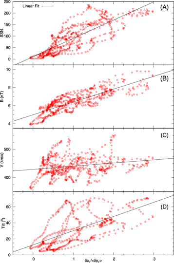
Figure 7. Correlations between the normalized force-field potential δϕ1 and SSN (panel (A)), the magnitude of the magnetic field B (panel (B)), the solar wind speed V (panel (C)), and the tilt angle of the HMF (panel (D)). The black lines show the least-squares fit. See text for an explanation.
Download figure:
Standard image High-resolution imageTable 3.
Correlation Coefficient and Linear Least-squares Fit for the Magnitude of the Magnetic Field, the Solar Wind Speed, the SSN, and the Tilt Angle of the HMF with Respect to the Normalized Force-field Modulation Potential (δϕ1/ )
)
| Parameter | a | b | Correlation | Variance of |
|---|---|---|---|---|
| Coefficient | Residuals | |||
| B | 1.42 ± 0.04 | 4.98 ± 0.05 | 0.8317 | 0.4 |
| V | 11.3 ± 2.0 | 429 ± 2 | 0.2224 | 1095 |
| SSN | 79.5 ± 2.2 | 10.5 ± 2.7 | 0.8212 | 1369 |
| Tilt | 17.7 ± 0.9 | 12.5 ± 1.2 | 0.6353 | 230 |
Download table as: ASCIITypeset image
The correlation coefficients of the regressions of δϕ1 versus SSN and B are 0.83 and 0.82, respectively. We consider these numbers as of secondary importance, however, and place more emphasis on the times and individual epochs where the correlation is good or weak. The best example of this point is solar cycle 20, which lasted from about 1965 to 1975 (see panels (A) and (C) of Figure 5). There is little solar cycle variation in B, but the modulation changes significantly. The anomalous behavior of B in the solar cycle is well known, and it is accepted as real. These space measurements have been confirmed by independent measurements of the so-called inter-diurnal variation of the geomagnetic field by Svalgaard & Cliver (2010).
This poor correlation for one of five cycles suggests that B alone is not a reliable proxy for cosmic-ray modulation. Steinhilber et al. (2010) suggested that the solar wind speed is also necessary to use B as a proxy (see their Equation (3)). The question also arises why it should be. Even the simplified theories of Section 2 do not predict it, and changes in δϕ and B are more likely due to other physical mechanisms. The argument may be that the amount of turbulence in B is a better indicator of κ.
4.4. Correlation: Force-field Potential and Modulation Parameters from Scattering Theory
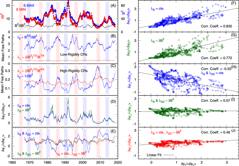
Figure 8 shows the solar cycle dependence of the mean free paths according to Equations (12) (panel (B)) and (13) (panel (C)). The ratio  (black line in panel (A)) shows a solar cycle variation, and this will influence the mean free path variations we present in panels (B)–(E). For low-rigidity cosmic rays, the parallel mean free path displays a well-defined solar cycle variation (in blue), which is higher at solar minimum than at solar maximum, as expected. For the perpendicular mean free path, there is no solar cycle dependence. For high-rigidity cosmic rays, the parallel mean free path is again higher at solar minimum than at solar maximum. The exception of this time variation for the parallel mean free paths is the interval around the solar maximum of 1969 when its value was high. Although the perpendicular mean free path shows a time variation, it is not clear, as for the case of the parallel one. This behavior may indicate that the parallel mean free path will show some correlation with cosmic-ray intensity, while the perpendicular mean free path will have a lack of correlation.
Figure 8. Left panels: 12-month moving averages of the square of B (in blue, panel (A), right vertical axis), magnetic field variance (δB2) (in blue, panel (A)), ratio of the square of B to the magnetic variance (in black, panel (A), left axis); mean free paths for low-rigidity cosmic rays (panel (B)) and high-rigidity ones (panel (C)); variations associated with the modulation parameter ψ∥ (panel (D)), and to ψ⊥ (panel (E)). Right panels: correlations of the normalized force-field potential δϕ1 with the modulation parameter δψ∥ (panels (F) and G), and δψ⊥ (panels (H), (I) and (J)). The black lines show the least-squares fit. See text for an explanation.
Download figure:
Standard image High-resolution image
Now we come to the point: How do these modulation parameters compare with those obtained from scattering theory in Equations (13) and (14)? To answer this question, we first have to rewrite the right-hand side of Equation (6) and normalized its value to that in March 1987. We represent this parameter with a different letter: ψ. It follows as
where the subscript "e" refers to the value at Earth. Now, assuming that V(r, t) = Ve(t), κ1(r, t) = κe(t) r (see, e.g., Moloto et al. 2018), and if we define the averages of δψe over the entire period as
  , then using the relation between diffusion coefficient and mean free path, κ = vλ/3 (v is the particle speed), we can rewrite Equation (17) for the normalized parameter
  as
as

From here all the analysis is referred to the Earth values, therefore the subscript "e" is omitted. The expression for the normalized modulation parameter in Equation (17) must be compared to the normalized values of δϕ for the three cases shown in Figure 6. We consider all cases in Equations (13)–(15), which lead to the normalized modulation parameters δψ∥/ and δψ⊥/
 , for the parallel and perpendicular mean free paths, respectively.
These new quantities are shown in panels (D) and (E) of Figure 8. δψ∥ (panel (D)) shows no difference between the two cases with (and without) solar cycle variations in the slab correlation scale. In general, δψ∥ is larger around solar maximum (or about two years after the maximum) than at solar minimum. At the same time, the variations in δψ⊥ are different for these two cases (blue and green lines). More importantly, none of them shows a higher value at solar maximum than at solar minimum, as we should expect from modulation theory. Because we wish to consider all reasonable options, we also analyzed the case described by Equation (15), where the slab correlation scale does not have solar cycle dependence and the 2D correlation scale does (shown in red, panel (E)). However, it is very similar to the case when both correlation scales are ∝δB2, which is an indication that variations in the slab correlation scale do not significantly contribute to the perpendicular mean free paths either.
As we proceeded with δϕ2 and δϕ2/3, for the correlation between δϕ1 and the parameters δψ∥ and δψ⊥, we used a linear relationship. This is because all these parameters are different estimates of the same physical quantity: the force-field modulation parameter appears in Equation (6).
The right panels of Figure 8 display one of the main results of the paper: the correlations of δϕ1 with different combinations of V, B, and δB2 as determined by our theories in Section 3. The correlation coefficient and the least-squares fit are listed in Table 4. The correlation of δψ∥ with the modulation potential from the force-field model is good: r = 0.83 and 0.77 for the two cases analyzed here. This new modulation parameter δψ∥ combines fluctuations in B2,  , and solar wind speed V. It is relevant to note that this complex parameter includes both modulation model and scattering theory. As we can see from panel (F) in Figure 8, there is a linear relationship between these two parameters, and this means that for long-term modulation, λ∥ in Equation (13) could be a proxy for the effective diffusion coefficient κ as employed in the force-field approach and therefore for the cosmic-ray variations. For the case shown in panel (G), the correlation is worse than in panel (F).
Table 4.
Correlation Coefficient and Linear Least-squares Fit for δψ∥/ and δψ⊥/
 with Respect to the Normalized Force-field Modulation Potential (δϕ1/
 )
)
| Parameter | a | b | Correlation | Variance of |
|---|---|---|---|---|
| Coefficient | Residuals | |||
![${[\delta {\psi }_{\parallel }/\langle \delta {\psi }_{\parallel }\rangle ]}_{{\lambda }_{S}=\mathrm{cte}.}$](https://content.cld.iop.org/journals/0004-637X/883/1/73/revision1/apjab3c57ieqn29.gif)
|
0.87 ± 0.02 | 0.12 ± 0.03 | 0.8343 | 0.15 |
![${[\delta {\psi }_{\parallel }/\langle \delta {\psi }_{\parallel }\rangle ]}_{{\lambda }_{S}\propto \delta {B}^{2}}$](https://content.cld.iop.org/journals/0004-637X/883/1/73/revision1/apjab3c57ieqn30.gif)
|
1.06 ± 0.04 | −0.07 ± 0.04 | 0.7711 | 0.35 |
![$[\delta {\psi }_{\perp }/\langle \delta {\psi }_{\perp }\rangle {]}_{{\lambda }_{2{\rm{D}}}=\mathrm{cte}.}^{{\lambda }_{S}=\mathrm{cte}.}$](https://content.cld.iop.org/journals/0004-637X/883/1/73/revision1/apjab3c57ieqn31.gif)
|
−0.78 ± 0.05 | 1.78 ± 0.06 | −0.5545 | 0.62 |
![$[\delta {\psi }_{\perp }/\langle \delta {\psi }_{\perp }\rangle {]}_{{\lambda }_{2{\rm{D}}}\propto \delta {B}^{2}}^{{\lambda }_{S}\propto \delta {B}^{2}}$](https://content.cld.iop.org/journals/0004-637X/883/1/73/revision1/apjab3c57ieqn32.gif)
|
0.03 ± 0.02 | 0.96 ± 0.02 | 0.0656 | 0.11 |
![$[\delta {\psi }_{\perp }/\langle \delta {\psi }_{\perp }\rangle {]}_{{\lambda }_{2{\rm{D}}}\propto \delta {B}^{2}}^{{\lambda }_{S}=\mathrm{cte}.}$](https://content.cld.iop.org/journals/0004-637X/883/1/73/revision1/apjab3c57ieqn33.gif)
|
0.19 ± 0.02 | 0.81 ± 0.02 | 0.4588 | 0.06 |
Download table as: ASCIITypeset image
In the case of δψ⊥, the correlation is shown in panels (H), (I), and (J) of Figure 8. We see that the correlation coefficient is higher (−0.55) when both correlation scales are independent of time, but it is an anticorrelation, opposite to what it is expected from cosmic-ray modulation. Moreover, the linear fit is very poor. The case with correlation scales ∝δB2 (panel (I)) is uncorrelated with δϕ1, and in the case when only the 2D correlation scale varies with time, δψ⊥ only shows a small correlation with δϕ1. In general, we should say that there is no solar cycle dependence on the perpendicular mean free path, or that it is not as strong as expected. Another possibility is that the solar cycle dependence of the turbulent scale λ2D is not yet fully understood, and therefore its contribution was not correctly taken into account in Equations (13) and (14). This is a point for future analysis.
4.5. Other Considerations beyond the Force-field Approximation
Improvements of the correlations may be sought in other parameters that do not appear in the simplified force-field theory. They are (a) changes in the size of the heliosphere, (b) the effects of gradient and curvature drifts, (c) nonspherically symmetric effects, and (d) episodic effects such as solar flares, coronal mass ejections, corotating interaction regions, merged interactions regions, and globally merged interaction regions.
Changes in the size of the heliosphere are probably not important in modulation variations. The Voyager space mission has indicated that radial gradients are proportional to r−a with 0 < a < 1 (Cummings et al. 1987). This implies from Equation (3) that  . For a = 1, Equation (6) shows that ϕ is proportional to rb if a = 0, and proportional to ln rb if a = 1. There are no indications that rb changes significantly over a solar cycle, while parameters such B and δBN, and therefore κ, can change by a factor of 3.
The role of curvature and gradient drift in the modulation has been emphasized since the theory was properly described by Jokipii et al. (1977). A commonly used measure of the relative importance of this effect is the tilt angle of the wavy neutral sheet that separates the inward- and outward-pointing magnetic fields (Hoeksema 1995). When the tilt is small at solar minimum, drifts should be relatively strong to determine the modulation depth, and when the tilt is large at solar maximum, it should be correspondingly weaker (Potgieter 1993). For this reason, many studies have correlated the modulation with the tilt angle of the wavy neutral sheet. Our current example is shown in Figures 5 and 7. From this, we make the following observations: (a) the correlation is not better than with sunspots; (b) it is significantly worse than the correlation with B2 and  throughout δψ∥ in Figure 8, and (c) there is no 22 yr or double solar cycle effect. The drift theory predicts such an effect because from one 11 yr cycle to the next, the drift directions in the heliosphere should reverse because of the reversing magnetic field. If drifts made a strong contribution, this implies that our correlations, which exclude the effect, should be different during successive solar minima. This effect cannot be seen in any of our correlation figures.
The nonspherically symmetric effects are relevant when we analyze the observations at different positions in the heliosphere. However, the Voyager observations in the outer heliosphere show that the radial intensity gradients dominate the latitudinal gradients (see, e.g., Caballero-Lopez et al. 2004b), therefore we consider the nonspherically effects as the second-order effect in the long-term modulation. Episodic effects such as solar flares, coronal mass ejections, corotating interaction regions, merged interactions regions, and globally merged interaction regions play a relevant role mainly at solar maximum. Most of the larger variations in cosmic-ray intensity at this period are associated with the large Forbush decreases (like in 1991 June). In other words, the effects of large solar events must be considered during the solar maximum epochs.
5. Summary
As we can see from Figure 6 (right panels) and Table 2, the correlation between NM counts and δϕ/ is very good and in agreement with previously reported studies (see, e.g., Usoskin et al. 2017; Santiago et al. 2018). At the same time, we found that different rigidity dependences on the diffusion coefficient give very similar results for the force-field modulation parameter, and all of the three cases analyzed in the present study could explain the NM observations and are very well correlated among each other. We should note that these high correlations are expected from the fact that we used the counting rate to compute the modulation parameter δϕ. We think that δϕ1/
 is more convenient as a reference because it is the most frequently used parameter and is easier to understand because it is a potential. However, the other rigidity dependences (P2 and P2/3) on the mean free paths in Equation (13) also give very good results with the force-field model, and moreover, they are supported by recent scattering theories. Therefore they are very suitable for modulation studies.
Although the long-term cosmic-ray variations are in agreement with solar cycle variations in SSN, the correlation between δϕ and SSN is worse than with the magnitude of the magnetic field B (Figure 7). The relations with the solar wind speed and the tilt angle of the HMF is not good. We consider that the fluctuations in these parameters alone do not explain the long-term modulation and therefore could not be used as a proxy for this type of studies.
One of the main aims of the present work was to investigate how the new insights from scattering theory could be used for long-term modulation, in particular, if we can use them with the simple force-field approximation. Our results show that the solar cycle dependence on the parallel mean free path is well correlated with the force-field modulation potential (and other rigidity dependences) in Equation (6). Therefore it is a good proxy for the effective diffusion coefficient, as subject to the approximations implicit to the force-field approximation, for long-term modulation studies.
The scenario with the perpendicular mean free path fluctuation is different. This parameter (as shown in Equations (13) and (14)) does not show a solar cycle dependence. When we assume that λ2D ∝ δB2, δψ⊥ is not anticorrelated with δϕ, but its correlation is very small. Our conclusion is that because the force-field approximation is an integrated model (Equation (6)), the magnetic field variations at 1 au are changing while fluctuations move away from the Sun, and therefore they cannot properly be taken into account within this cosmic-ray modulation model. All three cases for δψ⊥ analyzed here in the context of the force-field approximation do make a little difference, as opposed to the case where only their rigidity dependences are considered, but this difference leads to a lack of correlations that makes no sense in the light of what is known of the HMF geometry and its effect on cosmic-ray transport, as well as what is seen when 3D modulation codes are used (see, e.g., Engelbrecht & Burger 2015b; Moloto et al. 2018). Therefore, to extract information about modulation-related quantities from historical cosmic-ray data, one needs to take a more sophisticated approach to the Parker transport particle equation (see, e.g., Caballero-Lopez et al. 2004a).
As the main conclusion of this work, we consider that the long-term cosmic-ray modulation is properly described by the force-field modulation model with an effective diffusion coefficient with dependences similar to those of the parallel diffusion coefficients predicted by scattering theory (Equation (13)). With respect to the rigidity dependence on the mean free path, we think that all three cases analyzed here are suitable, ∝P and from scattering theory (∝P2 and ∝P2/3). As an integrated model, the force-field approximation is not able to precisely take into account the effects of 3D particle transport, and thus the effects of variations in the perpendicular diffusion coefficient resulting from changing turbulence quantities are not so great. In the future, it is important to investigate in detail the solar cycle dependence on the turbulence scale of λ2D, and to extend more advanced 3D cosmic-ray modulation codes, such as those of Qin & Shen (2017) and Moloto et al. (2018), to model the long-term modulation of galactic cosmic rays.
R.A.C.L.'s contribution was made during the sabbatical leave supported by a PASPA-DGAPA-UNAM grant. N.E.E.'s contribution is based on research supported in part by the National Research Foundation of South Africa (grant No. 111731). The opinions expressed and conclusions arrived at are those of the authors and are not necessarily to be attributed to the NRF. N.E.E. would like to thank R.A. Burger for valuable discussions on this subject. We acknowledge the use of NASA/GSFC's Space Physics Data Facility's OMNIWeb (or CDAWeb or ftp) service, and OMNI data. This work is dedicated to the memory of Professor Harm Moraal.