


Abstract
We seek to understand the quantitative role of the dominant physical processes (charge-exchange, adiabatic heating, stochastic acceleration) governing the proton distribution in the heliotail using observations of hydrogen energetic neutral atoms (ENAs) from the Interstellar Boundary Explorer (IBEX ). We solve the Parker transport equation for solar wind protons and pickup ions (PUIs) as they propagate from the termination shock (TS) down the heliotail, including charge-exchange between protons and neutral hydrogen atoms as source terms derived from an MHD-fluid and kinetic-neutral simulation of the heliosphere. We compute ENA fluxes at 1 au from the results of the proton transport model and compare them with IBEX observations. We find that, under the assumptions of our model, a stochastic acceleration process is needed to counteract the energy-dependent losses of ∼0.1–5 keV PUIs from charge-exchange to reproduce IBEX data. The power-law velocity dependence of the diffusion coefficient (spectral index γ) is limited to the range 0.67 < γ < 2, and the best fit to IBEX data appears close to γ ∼ 1.25. The diffusion rate ∼1.1 × 10⁻⁸ km2 s−3 (v/v0)1.25 nearly balances the loss of ∼0.1–5 keV PUIs by charge-exchange. Our analysis suggests that cyclotron resonance with two widely known incompressible MHD turbulence: namely, isotropic Kolmogorov and anisotropic Goldreich–Sridhar turbulence, as well as stochastic particle interactions with compressive waves are not by themselves the dominant diffusion mechanisms. However, some intermediate processes may be occurring due to the presence of PUIs.
Export citation and abstract BibTeX RIS
1. Introduction
The Interstellar Boundary Explorer (IBEX; McComas et al. 2009a) is an Earth-orbiting spacecraft that detects neutral atoms (mainly hydrogen) coming from the outer heliosphere (McComas et al. 2009b). These neutral atoms originate from the very local interstellar medium (VLISM; e.g., Möbius et al. 2009; Bochsler et al. 2012; Rodríguez Moreno et al. 2013; also see the review in McComas et al. 2017a) or are produced by charge-exchange between solar wind (SW) ions and interstellar neutral atoms in the inner heliosheath (IHS), creating energetic neutral atoms (ENAs; Gruntman et al. 2001; Heerikhuisen et al. 2008, 2014; Prested et al. 2008; McComas et al. 2009b; also see review in Zank 2015). The hydrogen ENA fluxes observed by IBEX depend on the properties of the plasma and neutral atom populations in different regions of the heliosphere and on how these populations interact (e.g., Zank 1999). For example, ENA observations from look directions just below the nose of the heliosphere show higher intensity compared with the flanks (Schwadron et al. 2011, 2014; McComas & Schwadron 2014), due to a larger energetic pickup ion (PUI) pressure and differences in the plasma flow vectors in different parts of the IHS (Zirnstein et al. 2016a). There is also an enhancement of ENA fluxes from look directions near the heliotail (i.e., downwind of the VLISM inflow direction), due to the greater depth of the ENA source region (e.g., Schwadron et al. 2014; Zirnstein et al. 2016a, 2017).
Figure 1 shows the ENA spectrum at ∼0.01–5 keV observed by IBEX from the downwind direction of the heliosphere. Fuselier et al. (2014) and Galli et al. (2016, 2017) suggest that there may be a rollover in the ENA spectrum below ∼0.1 keV from look directions near the heliotail. However, because the uncertainties in the observed ENA fluxes below ∼0.1 keV are very large (see the lowest three data points in Figure 1), we do not know whether the ENA spectrum rolls over, flattens, or continues to increase at lower energies. Validating this characteristic may help us understand the physical processes governing the evolution of the plasma distribution in the heliotail. Galli et al. (2016) further calculated an ENA source region "thickness" of a few hundred au (220 ±110 au) by converting the ENA fluxes to a line-of-sight partial plasma pressure, then Galli et al. (2017) extended this with a larger data set to find a lower limit of ∼280 au. However, this thickness should not be interpreted as the physical distance from the termination shock (TS) to the heliopause (i.e., physical thickness of the IHS in the downwind direction), but rather the line-of-sight integrated distance at which the majority of ∼0.1–1 keV ENAs are produced. Furthermore, if the ENA spectrum does not roll over, but continues to increase, then the inferred thickness of the ENA source region will be larger.

Figure 1. ENA fluxes from the VLISM downwind direction observed by IBEX. IBEX-Lo (blue) and IBEX-Hi (green) data are weight time-averaged from 2009 to 2012 using the methodology from Galli et al. (2017), and averaged over pixels in ecliptic longitude 48°–96° and latitude −12° to 12°. Note that the three lowest energy data points are consistent with zero flux and have large uncertainties (dashed lines). Therefore, we do not include these three data points in our analyses.
Download figure:
Standard image High-resolution imageOne aspect complicating the observation of low energy ENAs from the heliotail is that the source plasma is receding from us. Global models suggest the plasma flow speed is ∼100 km s−1 close to the TS, decreasing and then leveling out at ∼30 km s−1 beyond ∼400 au from the TS (see Appendix B). Hence, an ENA observed at 50 eV (100 km s−1) would have had an energy between 90 and 210 eV (130 and 200 km s−1) in the plasma frame.
The characteristics of the ENA spectrum from the heliotail also depend on the competing energy-dependent processes affecting the evolution of the proton distribution. Adiabatic heating of PUIs can occur due to, e.g., the compression of the subsonic flow by charge-exchange with interstellar neutral atoms (e.g., Czechowski & Grzedzielski 1995; Khabibrakhmanov & Summers 1996) or external forces from the VLISM, or perhaps via first-order acceleration by compressive turbulence in thermally isolated regions in space, i.e., the "pumping" mechanism (e.g., Fisk & Gloeckler 2014). The charge-exchange cross section is energy-dependent (Lindsay & Stebbings 2005), and the charge-exchange rate increases with energy up to ∼10–20 keV (Zirnstein & McComas 2015, Figure 2). Charge-exchange preferentially removes high-energy protons and replaces them with PUIs at the relative speed of the neutral and plasma populations, which is typically ∼0.1 keV in the heliosheath. Several physical processes have been associated with velocity diffusion, e.g., cyclotron resonant wave-particle interactions with an ambient wave field (e.g., Isenberg 1987, 2005; Chalov et al. 1997, 2003), particle interactions with compressive fluctuations in the SW plasma (e.g., Toptyghin 1980; Bykov & Toptygin 1993; Chalov et al. 2003, 2007; le Roux et al. 2005; Zhang & Lee 2013), acceleration at quasi-perpendicular interplanetary shocks (e.g., Giacalone et al. 1994; Lee et al. 1996; Zank et al. 1996), and acceleration via transit-time damping of compressive fluctuations in co-rotating interaction regions (e.g., Fisk 1976; Schwadron et al. 1996). In the heliotail, however, it is more difficult to determine which type of processes are governing the evolution of the plasma, due to the lack of in situ data. Voyager observations near the front of the heliosphere have shown evidence for compressive turbulence in the heliosheath plasma (Richardson & Burlaga 2013), which may also exist in the heliotail.
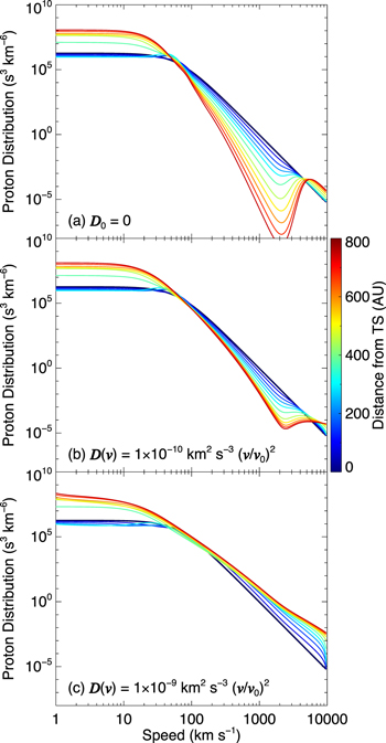
Figure 2. Evolution of the proton distribution assuming three different cases for velocity diffusion: (a) D0 = 0 (no velocity diffusion), (b) D(v) = 1 × 10⁻¹⁰ [km2 s−3] × (v/v0)2, and (c) D(v) = 1 × 10⁻⁹ [km2 s−3] × (v/v0)2. The initial distribution downstream of the TS is plotted in black (kappa distribution, where κ = 1.63). As the distribution evolves, its position is denoted by the color bar.
Download figure:
Standard image High-resolution imageThe physical structure of the heliotail is also a point of contention within the heliosphere modeling community. One model suggests that the heliotail is significantly shorter than the classical comet-like shape originally proposed by Parker (1961), due to the collimation of the SW plasma by the solar magnetic field tension force creating a physical split in the heliotail and its dissipation due to the growth of MHD-plasma instabilities (Opher et al. 2015). A recent analysis of Cassini/INCA data suggests the heliosphere might be spherical, possibly due to compression by a strong external interstellar magnetic field, thereby reducing the length of the heliotail (Dialynas et al. 2017). However, IBEX observations support the idea that the heliotail can be quite long (McComas et al. 2013; Pogorelov et al. 2017; Zirnstein et al. 2017), even though this is not manifested in a high ENA flux from the heliotail as might be expected for such a long column depth. The reason why IBEX does not observe significantly more ∼keV ENAs from the heliotail than the nose is because that energetic protons processed and transmitted across the TS are quickly lost due to energy-dependent charge-exchange, and are replaced by lower-energy PUIs (e.g., Schwadron et al. 2014; Siewert et al. 2014; Zirnstein et al. 2016a, 2017). Second, the single lobe ENA feature observed by IBEX from the heliotail at energies <2 keV and the two-lobed ENA feature observed at ENA energies >2 keV reflects the differences in the thermodynamic properties of the latitudinal-dependent SW (McComas et al. 2013; Zirnstein et al. 2016a). However, while this connection was recently supported by simulations (Zirnstein et al. 2017), simulated fluxes still underestimate the observations by a factor of ∼2–3. Therefore, a more careful study of the PUI evolution in the heliotail may help to better connect the ENA data to the global structure of the heliosphere.
In the following sections, we present a transport model of the proton distribution in the heliotail, by including effects of adiabatic heating by compression of the bulk flow due to charge-exchange; the energy-dependent injection and loss of protons by charge-exchange; as well as stochastic velocity diffusion, and calculate the ENA spectrum at 1 au produced from this model. We compare our model results to IBEX observations and determine the significance of these processes in evolving the proton distribution.
2. Model of Proton Distribution in the IHS
2.1. Transport Equation
We solve the stationary Parker transport equation with charge-exchange source terms in the IHS, under the assumption that the PUIs are advected with the bulk plasma, protons experience adiabatic acceleration and velocity diffusion, and include the production and loss of protons due to charge-exchange with neutral hydrogen:
where v is the proton velocity in the plasma frame, up is the bulk flow speed along the streamline distance coordinate s, fp is the proton distribution function (assumed to be isotropic in the plasma frame), D(v) is the velocity diffusion coefficient,  is the flow divergence term associated with adiabatic energy change, P is the production (source) term due to charge-exchange (photoionization is negligible, and electron-impact ionization is ignored in this study, see Section 2.2), and L is the loss (sink) term due to charge-exchange with neutral hydrogen atoms. The plasma flow speed and neutral hydrogen distribution used to calculate the charge-exchange source terms, both as a function of distance from the TS, are taken from our MHD-plasma/kinetic-neutral simulation of the heliosphere (Zirnstein et al. 2016b).
We ignore the spatial diffusion of PUIs, since the scale size of the heliosphere is much larger than the diffusion scale of ∼keV PUIs, or, equivalently, the diffusion time is much larger than the advection time (see also Fahr & Lay 2000; Fahr & Scherer 2004). We test different velocity diffusion coefficients of the form D(v) = D0 (v/v0)γ, where D0 is the diffusion rate amplitude, γ is the velocity spectral index, v is the particle speed, and v0 = 1 km s−1 is a normalization velocity, and D0 and D have units of km2 s−3. For the majority of the study, the parameters D0, v0, and γ are held constant through the IHS. However, in Section 4.1.2 we relax this assumption and allow D0 to change with distance to test the effects of a varying diffusion rate on ENA fluxes at 1 au.
2.2. Charge-exchange Source Terms
Following, e.g., Malama et al. (2006), we assume that the proton distribution function is isotropic in the plasma frame. The charge-exchange production and loss terms are given by
where the rates of ionization (η, β) are
where σex is the energy-dependent, charge-exchange cross section from Lindsay & Stebbings (2005). Charge-exchange and photoionization are included in the heliosphere simulation; however, at distances beyond the TS (≳100 au from the Sun) photoionization is practically negligible, so we ignore its effects when solving Equation (1). If electrons in the IHS have a significant thermal speed (e.g., Fahr et al. 2015), they may contribute to the ionization of neutral hydrogen in the heliosheath (e.g., Gruntman 2015). However, the only in situ observations of electrons in the IHS suggest the electron temperature downstream of the TS is insignificant (Richardson 2008; Richardson et al. 2008), and thus, ineffective for impact ionization. Therefore, we ignore electron-impact ionization in our calculations, though this effect could be included in future studies.
It is challenging to solve the proton transport equation, even one as simple as Equation (1), due to the computationally intensive integrals in Equations (2) and (3). This is why most global models of the heliosphere make assumptions for the proton distribution function (e.g., isotropic Maxwell–Boltzmann or kappa distribution) when computing the charge-exchange source terms in the MHD equations (e.g., Pauls et al. 1995; Heerikhuisen et al. 2008; Izmodenov et al. 2009; Opher et al. 2009; Pogorelov et al. 2016). However, in reality the proton distribution function in space plasmas is not Maxwell–Boltzmann, and is more kappa-like (e.g., Livadiotis 2015), although in the presence of charge-exchange is not necessarily a kappa distribution (e.g., Zirnstein & McComas 2015). Due to the large charge-exchange mean free path of neutral hydrogen in the heliosphere (e.g., Baranov & Malama 1993), the total neutral hydrogen distribution function in the IHS is also not Maxwell–Boltzmann and not likely to be isotropic; however, the majority of the neutral hydrogen density in the heliotail is from hydrogen atoms that originate in the VLISM or outer heliosheath (OHS). Models show that the velocity distributions of neutral atoms from the VLISM and OHS separately are close to Maxwell–Boltzmann (e.g., Izmodenov 2001; Heerikhuisen et al. 2006a); thus, we assume that the loss rate β in Equation (3) can be approximated by

with relative interaction speed (e.g., Pauls et al. 1995)
where nH is the local neutral hydrogen atom density, vth,H is the neutral thermal speed, and uH is the neutral bulk flow speed. Equation (4) represents a sum over the different neutral hydrogen species (i) which come from either the VLISM or the OHS. With this simplification, and the assumptions that the proton distribution function is isotropic in the plasma frame and the charge-exchange cross section is a slowly varying function of energy (Lindsay & Stebbings 2005), the loss term in Equation (2) is simplified to be
Equation (6) sums over neutral hydrogen atoms from the VLISM and OHS separately. The double integral in Equation (6) can be solved analytically, yielding
As stated earlier, the proton distribution is not Maxwell–Boltzmann, and while it is assumed to be a kappa distribution at the TS, under the action of charge-exchange the proton distribution does not necessarily remain kappa-like deeper into the heliotail (e.g., Zirnstein & McComas 2015; however, see Fahr et al. 2016 for a kappa-based model of IHS protons). In addition, velocity diffusion mechanisms and adiabatic heating will also change the shape of the distribution. To avoid making erroneous assumptions for the form of the proton distribution, we integrate the production rate of protons numerically using Equation (3) directly. Therefore, Equation (1) can now be written as
where P is solved by numerically integrating the production term in Equation (2), and the loss term L from Equation (2) has been solved analytically.
Global models of the heliosphere indicate that the neutral hydrogen density in the heliotail within ∼1000 au of the Sun is nearly constant, even slightly decreasing then increasing, as a function of distance from the Sun (e.g., Müller et al. 2008), and is dominated by neutral atoms from the VLISM and the OHS (e.g., Heerikhuisen et al. 2006a). Therefore, we utilize the results of a 3D, single-fluid MHD simulation of the heliosphere (Zirnstein et al. 2016b), which is coupled by charge-exchange to neutral hydrogen atoms solved using a Monte-Carlo approach (e.g., Heerikhuisen et al. 2006a, 2006b; Heerikhuisen & Pogorelov 2010) for our production and loss terms. We use the 6D phase space neutral hydrogen distribution produced by the simulation in the downwind direction of the simulated heliosphere as input for the charge-exchange production source term P in Equation (8).
2.3. Method of Solution—Finite Difference Method
We solve Equation (8) using an explicit, finite differencing scheme with a sufficiently small time-step such that the solution remains stable. Details on the methodology are described in Appendix A. We choose this method, rather than an implicit scheme (i.e., Crank–Nicolson method; e.g., le Roux & Ptuskin 1998; le Roux et al. 2007) or solving stochastic differential equations (e.g., Fichtner et al. 1996; Chalov et al. 2003; Senanayake et al. 2015), for its numerical simplicity in solving Equation (8). Velocity space can be solved in parallel on a multi-node computer cluster. Since the majority of the computation, for our purposes, is actually in the calculation of the nested production integral in Equation (3), this method of solution is sufficient compared to using an implicit scheme on a single computer node.
2.4. Initial Proton Distribution Downstream of the TS
For the proton distribution downstream of the TS, we assume the initial proton distribution function fp,0 is described by a kappa distribution (isotropic in the plasma frame) with initial density np,0, temperature Tp,0, and kappa index κp,0, written in the following form (e.g., Livadiotis & McComas 2013):
where  . We assume that the proton distribution processed by the TS is represented by a kappa distribution with kappa index slightly greater than 1.5 (e.g., Livadiotis et al. 2011), which is supported by other models (e.g., Fahr et al. 2014) and Voyager observations (Decker et al. 2005). The initial values for the parameters in Equation (9) are shown in Table 1, where np,0 and Tp,0 are based on our 3D MHD/kinetic simulation of the heliosphere (Zirnstein et al. 2016b). The plasma flow speed up and neutral hydrogen distribution fH as a function of distance from the TS are prescribed properties in our model and are taken from the results of the same heliosphere simulation mentioned previously. More details of this can be found in Appendix B. Note, however, that we also test different values for κp,0 in Section 4.1.3.
Table 1. Initial Parameters for the Proton Distribution Downstream of the TS
| Parameter | Value |
|---|---|
| Density, np,0 (cm−3) | 0.0017a |
| Temperature, Tp,0 (K) | 1.9 × 10⁶a |
| Kappa index, κp,0 | 1.63b |
Notes.
aDensity and temperature are taken from our MHD simulation (Zirnstein et al. 2016b). bKappa index taken from Voyager 1 observations downstream of the TS (Decker et al. 2005).Download table as: ASCIITypeset image
For the purposes of this study, we focus on the transport of protons down the heliotail including charge-exchange, adiabatic heating, and stochastic acceleration based on a single initial proton distribution (Equation (9)). In future studies, other distributions will be tested, e.g., multiple Maxwell–Boltzmann or filled-shell distributions (e.g., Vasyliunas & Siscoe 1976; Zank et al. 2010; Zirnstein et al. 2014, 2015, 2017), distributions based on more complex variations of PUI transport and processing in the supersonic SW (e.g., Isenberg 1987; Chalov et al. 1995, 1997; Schwadron et al. 1996; le Roux & Ptuskin 1998; Schwadron 1998; Fahr & Lay 2000; Fahr et al. 2007; Wu et al. 2016; Zank 2016), as well as distributions derived from particle-in-cell simulations of acceleration at the TS (e.g., Matsukiyo & Scholer 2014; Yang et al. 2015; Kumar et al. 2018).
Models of PUI transport should also be compared directly with observations of PUIs in the supersonic SW made by New Horizons' Solar Wind Around Pluto (SWAP) instrument (McComas et al. 2008, 2017b; Randol et al. 2012, 2013), which are the only direct observations of PUI distributions beyond ∼5 au from the Sun. McComas et al. (2017b) analyzed the interstellar hydrogen and helium PUI distributions from ∼20 to 38 au from the Sun, and found that the functional form of the isotropic, filled-shell distribution from Vasyliunas & Siscoe (1976) can be used to quantify the interstellar hydrogen and helium PUI distributions in the supersonic SW at ∼20–40 au from the Sun, but that the parameters of the distribution are not realistic most of the time in the vicinity of shocks or compressional waves. For the purposes of this paper, however, our model assumptions are reasonable based on our current knowledge of the proton distribution downstream of the TS at high energies from the Voyager spacecraft (e.g., Decker et al. 2005) and the inference that PUIs are likely heated and accelerated to higher energies at the TS (e.g., Zank et al. 1996, 2010; Richardson 2008; Yang et al. 2015; Kumar et al. 2018).
3. Results: Evolution of the Proton Distribution in the Heliotail
Figure 2 shows examples of the proton distribution as a function of distance from the TS down the center of the heliotail, where the initial distribution is defined by Equation (9) and parameters from Table 1. As one can see, the initial distribution fp,0 is a kappa distribution downstream of the TS, whose initial slope at high energies is given by  .
.
First, in the absence of velocity diffusion (Figure 2(a)), for the first ∼300 au from the TS the distribution does not change significantly at low speeds (<100 km s−1 ), except for a slight increase at ∼50 km s−1 in the plasma frame, which is approximately the relative injection speed for new PUIs (the flow speed is ∼70 km s−1 on average for the first 300 au, and the neutral hydrogen flow speed is ∼20 km s−1 in the same direction). However, after ∼400 au from the TS, the plasma slows and compresses (see Appendix B), resulting in an increased density, adiabatic heating, and injection of PUIs at lower speeds. At higher speeds (up to ∼3000 km s−1 ), energy-dependent charge-exchange removes a significant number of protons. At even higher speeds (>3000 km s−1 ), however, the charge-exchange cross section drops significantly (Lindsay & Stebbings 2005), reducing the chance for charge-exchange to occur. At these energies, heating by adiabatic compression occurs after 400 au from the TS.
When stochastic acceleration is included at a relatively low amplitude (Figure 2(b)), particles are accelerated to higher energies, partially countering the loss of ∼100–3000 km s−1 particles by charge-exchange. A stronger diffusion rate (Figure 2(c)) that is more efficient at accelerating particles to higher energies can counteract the charge-exchange loss rate. As we will show in Section 4, stochastic acceleration turns out to be a critical ingredient in the model in order to reproduce IBEX ENA observations.
4. Results: ENA Fluxes at 1 au and Comparison with IBEX Observations
In this section, we compute the line-of-sight integrated ENA flux at 1 au and compare the results to IBEX observations. The method for calculating ENA fluxes at 1 au can be found in many past studies (see e.g., Gruntman et al. 2001; Fahr & Scherer 2004; Zirnstein et al. 2013). As in our previous work (Zirnstein et al. 2013, 2015, 2017 and references therein), we smooth the model ENA spectrum over energy using a Gaussian function with full-width at half-maximum ΔE/E = 0.7, in order to approximately emulate the energy response function of the IBEX-Lo (Fuselier et al. 2009) and the IBEX-Hi (Funsten et al. 2009) sensors.
The results of the model for a variety of diffusion coefficient parameters are shown in Figure 3. We compare to IBEX data extracted from a group of pixels centered on the VLISM downwind flow direction. We statistically combine data from pixels between ecliptic longitude 48° and 96° and latitude −12° and 12°) using the methodology from Galli et al. (2017). The data have been corrected for background sources (see Galli et al. 2017 for details), transformed to the solar inertial frame, and corrected for the survival probability of ENAs inside 100 au (similar to our model).
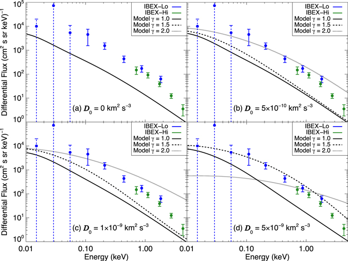
Figure 3. Comparison of model ENA fluxes at 1 au to IBEX observations for different diffusion coefficient parameters. Both the model and data are extracted from the VLISM downwind direction, i.e., the center of the heliotail.
Download figure:
Standard image High-resolution imageThe data are also weight-averaged over time from 2009 to 2012 to provide sufficient statistics and excludes the possible time-dependent fluxes found by Galli et al. (2017) after 2012. We model ENA fluxes from the VLISM downwind direction, i.e., the center of the angular range of the IBEX data.
4.1. Role of Velocity Diffusion in the Heliotail
Our first comparison to the data is for the case where there is no stochastic acceleration (D0 = 0). In this case, our modeled fluxes are lower than the data at all energies. We note that this discrepancy exists in our previous model of ENA fluxes from the heliotail when only charge-exchange effects are included (Zirnstein et al. 2017).
Figure 3 also shows model ENA fluxes when velocity diffusion was included for a range of diffusion spectral indices (1 ≤ γ ≤ 2) and diffusion coefficient amplitudes (0 ≤ D0 ≤5 × 10⁻⁹ km2 s−3). In general, more particles appear at higher energies when either D0 or γ increases, but the slope of the ENA spectrum depends strongly on the diffusion spectral index. As D0 increases for low γ (<1.5), ENA fluxes at low energies increase slightly, producing a steep ENA spectrum. However, as γ increases (>1.5), particles diffuse to higher energies, producing a significantly flatter spectrum. It might appear that there is a partial degeneracy in the diffusion coefficient parameters when comparing to IBEX data, so that we may be able to reproduce IBEX observations with a larger D0 and smaller γ, or smaller D0 with larger γ. However, this is not the case, and in Section 4.1.1, we will show how the range of likely diffusion coefficients can be narrowed down by performing a reduced chi-square analysis with IBEX data.
4.1.1. Velocity Diffusion Coefficient in the Heliotail Scales as ∼v1.25
Figure 4 shows the reduced chi-square values for a range of D0 when 0.67 ≤ γ ≤ 2. The results show that the "best-fit" diffusion spectral index lies 1.25. The reason for this is demonstrated in the right panel of Figure 4. For the case where the diffusion scales with velocity as ∼v0.67 or lower, the model ENA spectrum overestimates several of the low energy observations, indicating that this type of diffusion is not sufficient to diffuse particles to >1 keV energies. Similarly, the results for a diffusion rate scaling as ∼v2 or higher overestimates the diffusion of particles to higher energies and underestimates the flux at lower energies, creating an ENA spectrum that is too flat compared to IBEX observations. Thus, the diffusion spectral index lies in the range 1 ≲ γ ≲ 1.5, and it appears most likely to be close to γ ∼ 1.25 with D0 ∼ 10−8 km2 s−3. Figure 5 shows how the proton distribution evolves with distance through the heliotail when the diffusion coefficient D(v) = 1.125 × 10⁻⁸ km2 s−3 (v/v0)1.25. Comparing Figure 5 to the first panel in Figure 2, the rate of diffusion appears to nearly balance the loss of protons by charge-exchange in the speed range ∼100–1000 km s−1, which encompasses the IBEX ENA energy range.
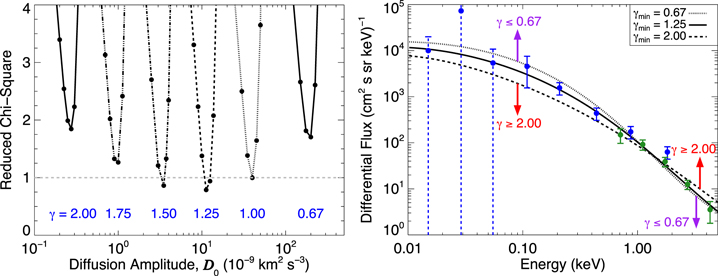
Figure 4. Left panel: reduced chi-square values for a range of diffusion amplitudes (D0) for 0.67 ≤ γ ≤ 2. Right panel: best-fit ENA flux results for γ = 0.67, 1.25, and 2 (i.e., D0 that produce minimum reduced chi-square for each γ). Note that as the spectral index γ increases ≳2 or decreases ≲0.67, the model ENA fluxes at 1 au cannot reproduce the observed low and high ENA fluxes simultaneously.
Download figure:
Standard image High-resolution image
Figure 5. Evolution of the proton distribution in the heliotail assuming the "best-fit" diffusion rate from Figure 4, D(v) = 1.125 × 10⁻⁸ km2 s−3 (v/v0)1.25.
Download figure:
Standard image High-resolution image4.1.2. Velocity Diffusion Rate May Slowly Vary with Distance from the TS
In this section, we relax our assumption that the diffusion rate remains constant for hundreds of au through the heliotail. The diffusion rate will most likely decrease as a function of distance from the TS if the acceleration mechanism is of solar origin and the amplitude of, e.g., magnetic fluctuations, dissipate with time. In Figure 6, we show different examples of the evolution of the diffusion rate: (1) D0 decreasing linearly with distance such that D0 = 0 at 800 au, (2) D0 decreasing linearly such that D0 = 0 at 400 au, and (3) D0 increasing linearly with distance such that D0 = 0 at the TS. We also show an example where D0 remains constant through the heliotail. For all cases, we assume γ = 1.25, and normalize D0 such that the average D0 over the simulation range is equal to 1.125 × 10⁻⁸ km2 s−3.
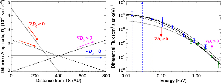
Figure 6. Left panel: diffusion rate amplitude as a function of distance from the TS, for four different cases (increasing diffusion rate—magenta, decreasing diffusion rate—red, or no change—blue). Their normalizations are chosen such that they have the same average diffusion rate over the 800 au simulation domain, 1.125 × 10⁻⁸ km2 s−3. Right panel: ENA fluxes at 1 au for the diffusion rate trends from the left panel.
Download figure:
Standard image High-resolution imageAs one can see, the model ENA spectra for the cases where D0 is constant and D0 decreases linearly at a slow rate (reaching D0 = 0 at 800 au) compare well to the data over all energies. However, when D0 decreases more quickly (the case where D0 = 0 at 400 au from the TS), the resulting ENA spectrum underestimates the observations at low energies.
It is also possible the diffusion rate increases with distance from the TS if (1) turbulence from the VLISM permeates the heliotail and increases the rate of diffusion (but still results in the same diffusion spectral index γ ∼ 1.25), or (2) the heliotail develops large-scale instabilities that may transfer turbulent energy to smaller scales. Figure 6 shows an example where D0 increases linearly with distance, with the same average diffusion amplitude as the other examples. It appears that a moderately fast increase in diffusion with distance from the TS results in an ENA spectrum that overestimates the data at high ENA energies. Therefore, we conclude that it is possible the diffusion coefficient decreases slowly with distance, and the average diffusion coefficient amplitude D0 can still be approximately 10−8 km2 s−3.
4.1.3. Dependence on the Proton Distribution Kappa Index at the TS
So far, we have modeled the proton distribution in the heliotail under the assumption that its initial kappa index κp,0 = 1.63. While this may be true for the distribution measured by Voyager 1 (Decker et al. 2005), it may be different in other locations. In this section, we briefly test how well the model ENA spectrum compares to IBEX observations if κp,0 is allowed to vary. Figure 7 shows model results for κp,0 = 1.51, 2, and 10. As one can see, for the diffusion coefficient D(v) = 1.125 × 10⁻⁸ km2 s−3 (v/v0)1.25, the model where κp,0 = 1.51 produces less flux at the highest energies compared to κp,0 = 2 and 10, similar to the results for κp,0 = 1.61 (see Figure 4, right panel). It appears that the results are not significantly sensitive to κp,0, at least for the diffusion coefficient we have derived, but it appears that a kappa index less than ∼2 is most consistent with the observations at the highest energies. In a future study, we will explore in more detail how κp,0 and other forms for the initial proton distribution depend on the velocity diffusion coefficient.

Figure 7. Comparison of IBEX observations and model ENA fluxes for different κp,0. We assume D(v) = 1.125 × 10⁻⁸ km2 s−3 (v/v0)1.25.
Download figure:
Standard image High-resolution image4.2. No Rollover in the ENA Spectrum from the Heliotail below ∼0.1 keV
It was suggested by Fuselier et al. (2014) and Galli et al. (2016) that the ENA spectrum from the heliotail may roll over at energies <0.1 keV. Our results suggest that the ENA spectrum does not roll over below ∼0.1 keV, although it may flatten (see, e.g., Figure 3). The reason for this behavior is that low energy PUIs are continually injected into the heliotail plasma from charge-exchange with neutral hydrogen propagating into the heliotail, and these PUIs are accelerated to higher energies. These PUIs eventually become ENAs that are observable by IBEX. A rollover in the ENA spectrum would suggest that IBEX could detect ENAs originating from the peak of the IHS proton distribution—but our results show this is not the case. One of the key factors for this is that we can only observe signatures of PUIs with an energy above ∼5–25 eV in the plasma frame, corresponding to flow speeds in the range ∼30–100 km s−1 (see Figure 5). Our results are still consistent with the analyses of Galli et al. (2016, 2017), who derived a maximum flux of ∼104 ENA/[cm2 s sr keV] at ENA energies <50 eV in the downwind hemisphere, and are consistent with the estimated upper limit of neutral hydrogen fluxes in the heliotail based on Lyα observations from the Hubble Space Telescope (Wood & Izmodenov 2010; see also Fuselier et al. 2014).
5. Discussion and Conclusion
In this paper, we seek to understand the dominant physical processes (charge-exchange, adiabatic heating, stochastic acceleration) governing the energy distribution of protons in the heliotail, and to understand their connection in forming the ENA spectrum from ∼0.05 to 5 keV observed by IBEX. To do this, we model the ENA spectrum from the VLISM downwind direction by solving the isotropic Parker transport equation for protons in the heliotail, including charge-exchange source terms and adiabatic heating derived from an MHD-plasma/kinetic-neutral simulation of the heliosphere, as well as velocity diffusion which we implement as a free parameter in order to fit to IBEX ENA observations.
Using IBEX ENA observations from the heliotail, we find that there is likely a form of energy diffusion of ∼0.1–5 keV protons in the heliotail. Without diffusion in energy, the model ENA fluxes underestimate the data by a factor ∼2–3 over all energies due to the fast rate of removal of high-energy protons by the energy-dependent, charge-exchange process. Therefore, the significant removal of high-energy protons (at energies <10 keV) by charge-exchange, the injection of low energy PUIs (∼0.1 keV), as well as moderate acceleration of low energy PUIs to higher energies are fundamental processes occurring in the IHS.
We find that the diffusion rate's spectral index lies in the range 1 ≲ γ ≲ 1.5, where a diffusion rate with amplitude ∼1.1 × 10⁻⁸ km2 s−3 that scales approximately as ∼v1.25 is most consistent with IBEX observations. For diffusion mechanisms with velocity dependences γ < 1, the resulting ENA spectrum becomes too steep compared to IBEX-Lo observations. Thus, our analysis suggests that an isotropic Kolmogorov turbulence (the power spectrum scaling as k−5/3), which gives a velocity diffusion rate scaling as v2/3 (e.g., Isenberg 1987) if the interaction of particles with the turbulent eddies is predominantly via cyclotron resonance, is likely not the primary diffusion mechanism for ∼0.1–5 keV PUIs in the heliotail. On the other hand, an anisotropic turbulence where the power spectrum along the local mean magnetic field is much steeper (e.g., Goldreich & Sridhar 1995; Boldyrev 2006; Kumar et al. 2017) produces a steeper dependence of the diffusion rate on v. For instance, an incompressible anisotropic turbulence may give D(v) ∝ v2 as suggested by Eichler (2014). But, our results suggest this is too steep to reproduce IBEX observations. It is possible, however, that the presence of PUIs alters the magnetic field turbulence in the heliotail. For example, if the anisotropic turbulence power is enhanced parallel to the magnetic field due to the presence of PUIs and the parallel power spectrum becomes flatter, then this may result in a lower diffusion spectral index. Moreover, there are also other commonly used mechanisms that, by themselves, produce diffusion coefficients that are too steep to reproduce IBEX data, such as stochastic particle interactions with large-scale fluctuations or compressive waves, which yield a diffusion coefficient D(v) ∝ v2 (e.g., Toptyghin 1980; Bykov & Toptygin 1993; Chalov et al. 1997, 2003; Chandran 2003; le Roux et al. 2005; Zhang 2010; Fahr et al. 2012; Zhang & Lee 2013).
Based on our analysis, there is not a rollover in the ENA spectrum below ∼0.1 keV, although the ENA spectrum may slightly flatten. ENAs that are observed by IBEX below ∼0.1 keV originate from low energy PUIs that were partially accelerated, possibly via stochastic diffusion. Galli et al. (2017) recently provided an updated analysis of low energy IBEX observations from the heliotail direction from 2009 to 2017. They show a potential rollover may still exist below ∼0.1 keV, and they also found a significant increase in 0.1–0.2 keV ENA fluxes compared to previous years, which may be a time-dependent effect. In a future study, we can compare our model to this updated data set, which may suggest a change in the diffusion coefficient or the initial conditions of the proton distribution function downstream of the TS.
The loss of ∼1–10 keV protons by charge-exchange steepens the PUI distribution function at energies below 10 keV and produces a bump in the distribution function at ∼50–100 keV (a few thousand km s−1, see Figure 2). The modified distribution function may be susceptible to various plasma instabilities, e.g., bump-in-tail instability. A quantitative study of these instabilities is beyond the scope of this paper. Nonetheless, the velocity diffusion of PUIs may directly be impacted if the instabilities can grow additional magnetic turbulence to a level comparable to the existing turbulence at a rate faster than the advection rate of SW plasma. Under such a scenario only the physical interpretation of the diffusion coefficient is modified since the velocity diffusion we derive is an independent component of our phenomenological model, which serves to adjust the PUI distribution function in order to reproduce the IBEX ENA observations. Moreover, regardless of not fully understanding the physical mechanism behind the acceleration of PUIs in the IHS, we are able to characterize the diffusion coefficient in future models of the IBEX ENA spectrum.
The authors thank the anonymous referee for valuable comments on the paper. E.Z. and J.H. acknowledge support from NASA grant NNX16AG83G. This work was also carried out as part of the IBEX mission, which is part of NASA's Explorer program. R.K. was partially supported by the Max-Planck/Princeton Center for Plasma Physics and NSF grant AST-1517638. E.Z. acknowledges helpful discussions with Jakobus le Roux. The work reported in this paper was performed at the TIGRESS High Performance Computing Center at Princeton University which is jointly supported by the Princeton Institute for Computational Science and Engineering and the Princeton University Office of Information Technology's Research Computing department.
Appendix A: Solving the Parker Transport Equation
In order to solve Equation (8), we first write it in natural logarithm space:
where w = ln(v). This yields a straightforward way to solve the transport equation with logarithmically spaced speed bins. We solve for speeds in the plasma frame ranging from 1 to 10,000 km s−1 (or ∼0.005–522 keV), where the speed bin sizes range from ∼0.03 to 300 km s−1, respectively.
We solve Equation (11) using an explicit, "forward-time, central-difference" method, which requires a sufficiently small step size Δs to remain stable. Thus, Equation (11) becomes (e.g., Press et al. 2002):
where n is the spatial (or time) step index (sn), j is the velocity step index (wj), Δs = sn+1 − sn, Δw = wj+1 – wj, Dj+1/2 =(Dj+1 + Dj)/2, Dj–1/2 = (Dj + Dj–1)/2, wj+1/2 = (wj+1 + wj)/2, and wj-1/2 = (wj + wj–1)/2. The production term P is solved by numerically integrating Equations (2) and (3). We solve Equation (12) using Equations (2), (3), (6), and (7) as a function of distance s = 0 to 800 au from the TS. The step size, Δs, is chosen such that it globally satisfies the stability condition, which is approximately given by (e.g., Press et al. 2002)
Appendix B: Simulation Properties in the Heliotail
A zeroth order estimate of the divergence of the plasma flow in the IHS, in the presence of charge-exchange, gives  , where β is the rate of charge-exchange and α is the adiabatic index (e.g., Czechowski & Grzedzielski 1995; Khabibrakhmanov & Summers 1996; Florinski et al. 2004). This term is negligible over small distances from the TS (Zirnstein & McComas 2015; Zirnstein et al. 2016a), but not over longer distances. However, we can calculate the flow divergence directly from our 3D MHD simulation, which self-consistently couples to neutral hydrogen through charge-exchange source terms. We find that the flow divergence in our simulation is much more complicated than the zeroth order assumption (see Figure 8). In fact, it is likely even more complicated in reality when the plasma flow velocity is changing over time due to short and long-term changes in the SW. Therefore, we smooth the MHD-derived divergence term, interpolate it to our spatial grid, and use it when solving the flow divergence term in Equation (12).

Figure 8. Proton bulk flow speed (left) and flow divergence (right) as a function of distance from the TS down the center of the heliotail, from an MHD-plasma and kinetic-neutral simulation of the heliosphere (Zirnstein et al. 2016b). Note that the flow divergence is erratic due to statistical noise from the charge-exchange source terms. Therefore, we smooth the results, and use the smoothed version (blue line) in our transport model of the proton distribution function.
Download figure:
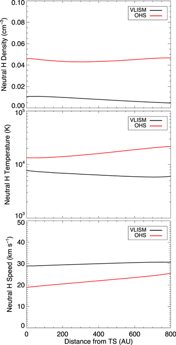
Standard image High-resolution imageThe neutral hydrogen density, temperature, and bulk flow speed from two different populations derived from our simulation of the heliosphere are shown in Figure 9. We account for neutral hydrogen originating from the pristine VLISM and the OHS in the charge-exchange source terms in Equation (11). Figure 9 shows that the density of neutral hydrogen from the OHS is higher than those from the VLISM, and it is practically constant in the heliotail (up to at least ∼1000 au from the Sun). The temperature of neutral hydrogen from the OHS is also higher, since they originate from VLISM protons that were compressed and heated at the bow shock/wave ahead of the heliosphere. Consequently, this means that neutral hydrogen atoms from the OHS are slower than those from the VLISM. While other studies show more significant changes to the neutral H populations beyond ∼1000 au from the Sun (e.g., Izmodenov & Alexashov 2003), the majority of ENAs observed at 1 au originate within a few hundred au of the TS.
Figure 9. Neutral hydrogen (H) density (top panel), temperature (middle panel), and flow speed (bottom panel) as a function of distance from the TS down the center of the heliotail, from an MHD-plasma and kinetic-neutral simulation of the heliosphere (Zirnstein et al. 2016b). We include neutral hydrogen from the VLISM and OHS in the charge-exchange source terms in our model.
Download figure:
Standard image High-resolution image