


Abstract
Comet C/2011 W3 (Lovejoy) is the first sungrazing comet in many years to survive perihelion passage. We report ultraviolet observations with the Ultraviolet Coronagraph Spectrometer (UVCS) spectrometer aboard the Solar and Heliospheric Observatory satellite at five heights as the comet approached the Sun. The brightest line, Lyα, shows dramatic variations in intensity, velocity centroid, and width during the observation at each height. We derive the outgassing rates and the abundances of N, O, and Si relative to H, and we estimate the effective diameter of the nucleus to be several hundred meters. We consider the effects of the large outgassing rate on the interaction between the cometary gas and the solar corona and find good qualitative agreement with the picture of a bow shock resulting from mass loading by cometary neutrals. We obtain estimates of the solar wind density, temperature, and speed, and compare them with predictions of a global magnetohydrodynamic simulation, finding qualitative agreement within our uncertainties. We also determine the sublimation rate of silicate dust in the comet's tail by comparing the visible brightness from the Large Angle Spectroscopic Coronagraphs with the Si iii intensity from UVCS. The sublimation rates lie between the predicted rates for olivines and pyroxenes, suggesting that the grains are composed of a mixture of those minerals.
Export citation and abstract BibTeX RIS
1. Introduction
A family of comets following similar orbits that pass extremely close to the surface of the Sun was recognized in the 1880s (Kirkwood 1880; Kreutz 1888), and they are now known as Kreutz sungrazers. Marsden (2005) reviews their history, and Sekanina & Chodas (2007) discuss the dynamics of nucleus breakup that could account for the distribution of sungrazers. More than 2600 of these sungrazers have been discovered in images from the Large Angle Spectroscopic Coronagraphs (LASCO) (Breuckner et al. 1995) aboard the Solar and Heliospheric Observatory (SOHO) satellite. Biesecker et al. (2002) and Knight et al. (2010) have examined their light curves, which peak at around 11 R☉ (R☉ = 0.00465 au) because dust grains reach such high temperatures close to the Sun that they vaporize rapidly. A comprehensive review of comets near the Sun is given by Jones et al. (2018).
The Ultraviolet Coronagraph Spectrometer (UVCS) aboard the SOHO satellite (Kohl et al. 1995, 1997) has observed several sungrazing comets in the past (Raymond et al. 1998; Uzzo et al. 2001; Bemporad et al. 2005; Ciaravella et al. 2010; Giordano et al. 2015) as well as a few ordinary comets near the Sun (Raymond et al. 2002; Povich et al. 2003). By far the brightest UV line is Lyα. It is formed when H2O photodissociation produces H atoms, which form an expanding cloud that resonantly scatters Lyα photons from the solar disk. The intensities provide estimates of the outgassing rates, which in turn give estimates of the nucleus diameter. Two of the sungrazers showed C iii and Si iii lines, which permitted estimates of the carbon and silicon abundances. It was also possible to determine coronal parameters from the observations. The Lyα line width and the expansion rate of the H i cloud give the coronal proton temperature along the comet trajectory, and the decay time of the Lyα brightness is the H i ionization time, giving the coronal electron density. Unlike most remote sensing measurements, these comet observations probe the coronal conditions at points along the comet trajectory, rather than giving average quantities along the line of sight (LOS).
Comet Lovejoy (C/2011 W3) was discovered by Terry Lovejoy on 2011 November 27. It was the brightest sungrazing comet observed in recent years, and its orbit was predicted well in advance (Lovejoy & Williams 2011), facilitating observations with UVCS. Its unusually large nucleus survived perihelion passage, though it broke up 1.6 days after perihelion (Sekanina & Chodas 2012). It was observed by the AIA instrument aboard the Solar Dynamic Observatory in the low corona, the second comet detected by AIA after Comet C/2011 N3 (Schrijver et al. 2012). Its emission in the EUV bands of AIA was dominated by lines of oxygen (Bryans & Pesnell 2012). It was also detected by the XRT and SOT instruments on the Hinode spacecraft. The AIA and XRT observations are discussed by McCauley et al. (2013), and Downs et al. (2013) used the AIA observations to investigate the structure of the coronal magnetic field. Raymond et al. (2014) extended the analysis of the AIA images to investigate the small-scale density structure of the corona and the pickup ion (PUI) behavior of the oxygen produced by the comet.
This paper concentrates on UV spectra and white light images of Comet Lovejoy obtained with the UVCS and LASCO instruments aboard the SOHO satellite during ingress at heliocentric distances between 2 and 10 R☉. Comet Lovejoy requires more complicated analysis than the other sungrazers observed by UVCS, because the high mass loss rate severely disturbs the ambient corona. We obtain estimates of the outgassing rate and size of the comet nucleus and the relative abundances of H, N, O, and Si. We also estimate the coronal densities and compare the densities, observed Doppler shifts, and line widths with those expected from the density and solar wind speeds predicted by the Magnetohydrodynamic (MHD) Algorithm outside a Sphere (MAS) global MHD model of the corona. In addition, we make a first attempt to determine the sublimation rate of silicate grains in the tail by comparing the visible light brightness and the intensity of the Si iii emission line.
2. Observations
2.1. UVCS
The UVCS instrument observed several sungrazing comets (Bemporad et al. 2007). The instrument is described by Kohl et al. (1995, 1997). Briefly, the 42' slit can be placed at any position angle around the Sun and at any height between 1.5 and 10 R☉. As with other comet observations, we placed the UVCS slit at a position determined from the predicted orbit of the comet, let the comet drift across the slit, then moved the slit to a lower height. We used the LYA channel to cover the spectral range 1200–1245 Å with the 100 μm slit, which provides about 140 km s−1 resolution. Figure 1 shows the slit positions superposed on LASCO C2 and C3 images of the comet.
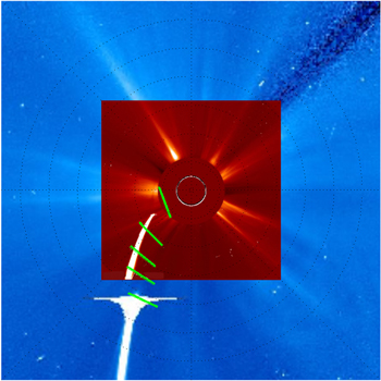
Figure 1. UVCS slit positions for the five observations of Comet Lovejoy. Positions and observing intervals are given in Table 1. Note that the trajectory of the nucleus passes closer to the center of the slit than does the dust tail in this image.
Download figure:
Standard image High-resolution imageThe slit positions and observing times were chosen to provide some exposures before the comet arrived and to cover the fading of the Lyα emission after the passage of the comet. However, the comet arrived somewhat before the predicted times, and a delay in the availability of near real time commanding caused the observing sequence to start late. Therefore, we had fewer exposures than desired before the peak comet brightness. A list of the observations is provided in Table 1. The start and stop times for the observations at each height are given in the first two columns, and the third column gives the time when the comet crossed the slit. The crossing times, which are 15–20 min earlier than those used to plan the observations, are based on an updated ephemeris. The fourth column gives the apparent distance from Sun center in the plane of the sky, RPOS, and the fifth column is the actual distance, R, including the displacement along the LOS based on the comet's orbit. Henceforth we will use the value of R to refer to each crossing of the slit. The heights refer to the lower edge of the UVCS slit, while the upper edge is 28'' higher. All times are UT on 2011 December 15 and 16. Table 1 also gives the position angle of the UVCS slit (degrees E of N), the comet speed, Vcom, the line-of-sight speed, VLOS, the radial speed, VR, and the phase angle according to the comet ephemeris.
Table 1. UVCS Slit Positions
| tstart | tstop | tcross | RPOS | R | PA | Vcom | VLOS | VR | ϕ |
|---|---|---|---|---|---|---|---|---|---|
| 16:26 | 18:38 | 16:46 | 8.37 | 9.98 | 144.8 | 202 | 139 | 129 | 56 |
| 18:39 | 20:04 | 18:46 | 6.92 | 8.02 | 139.9 | 226 | 153 | 135 | 60 |
| 20:07 | 21:34 | 20:14 | 5.71 | 6.36 | 134.4 | 251 | 168 | 141 | 64 |
| 22:21 | 23:11 | 21:53 | 4.14 | 4.32 | 125.0 | 289 | 194 | 156 | 73 |
| 23:14 | 00:16 | 23:34 | 2.00 | 2.08 | 100.0 | 449 | 215 | 278 | −74 |
Download table as: ASCIITypeset image
The radiometric calibration of UVCS was determined in the laboratory before launch, then tracked through 2005 by observing an ensemble of stars that passed within a few degrees of the Sun during the course of the year (Gardner et al. 2002; Valcu et al. 2007). We used an observation of the star Theta Oph at 7.6 R☉ immediately prior to the comet observations and observations of the star Rho Leo between 3.1 and 8.0 R☉ from 2011 August to determine the calibration to apply to the observations of Comet Lovejoy. The radiometric calibration should be accurate to 15% or better.
The UVCS detectors had lost spatial resolution by the time of the Comet Lovejoy observations, in that counts from groups of eight rows were collapsed into single rows. We were therefore unable to measure the spatial extent of the comet emission. The detector also showed signs of degradation at the center of the Lyα line at some spatial positions. We corrected for that weaker response based on the Lyα profiles at 2 R☉ before the comet arrived, making the assumption that the intrinsic profile was the same at all positions, fitting Gaussians to the wings of the lines, and using the ratio of the fit to the measured count rate at line center. This correction is probably accurate to about 20%.
Figures 2 and 3 show two of the spectra. The first is the average of three exposures from 23:33:24 to 23:39:32 UT on December 15, when the comet crossed the slit at 2.1 R☉ minus the pre-comet background. The second is the average of 18 spectra from 23:29:36 to 00:16:44 UT after the comet had left the slit minus the average of nine spectra taken before the comet arrived. In this spectrum the oxygen has had time to reach the O4+ ionization state, and the background-subtracted Lyα is not as bright as when the comet was in the slit, so the O v] line in the wing can be better seen. The coronal Lyα line does not subtract off perfectly because it is Doppler shifted to the red due to the disturbance caused by the comet.
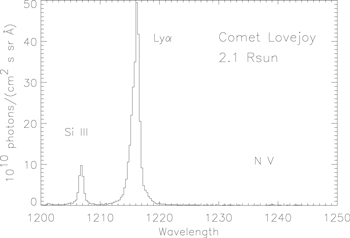
Figure 2. UVCS spectrum at 2.1 R☉ showing the Lyα and Si iii lines. This is the sum of three exposures of 120 s near peak Lyα brightness minus the average of nine exposures before the comet arrived.
Download figure:
Standard image High-resolution image
Figure 3. UVCS spectrum at 2.0 R☉ showing the N v and O v] lines along with the background coronal Lyα. This is the average of 18 exposures covering the time over which the lines brightened and faded away minus the average of nine exposures before the comet arrived.
Download figure:
Standard image High-resolution imageThe brightest spectral line is H i Lyα. Figures 4 through 6 show the time behavior of the Lyα intensity, line centroid, and line width for the crossings at 10, 8, 6.4 and 2.1 R☉. The data from the first part of the crossing at 4.14 R☉ are missing due to a telemetry loss, making the interpretation ambiguous, and we will not consider that crossing further. Because the comet arrived a little earlier than predicted and our observing sequence began later than predicted due to late acquisition of real-time commanding, we barely caught the peaks of the emission at 8 and 6.4 R☉. We caution that the apparent degradation of the detector near the line center means that both the centroids and widths should be treated with care. We have normalized the velocity scale to zero during the exposures at 2.1 R☉ before the comet arrived, but there is some possibility that the velocity differed from zero. The behavior shown is qualitatively correct, but both velocity shifts and line widths contain systematic errors that we have no solid way to determine. We estimate uncertainties of 20% in intensity and 50 km s−1 for line centroid and width, but we cannot verify these estimates.
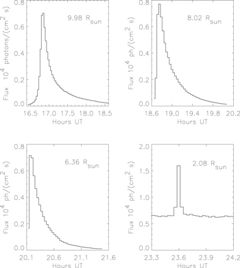
Figure 4. Lyα fluxes as a function of time for the four times that Comet Lovejoy crossed the UVCS slit. The fluxes are given in  at Earth. Systematic uncertainties in the intensities are estimated to be 15%–20%.
Download figure:
Standard image High-resolution image
Figure 5. Lyα velocity centroids as a function of time for the four times that Comet Lovejoy crossed the UVCS slit. The relative velocities at each height are reliable, but there may be some systematic velocity offset, Δ, as large as 50 km s−1.
Download figure:
Standard image High-resolution image2.2. LASCO
The optical brightness of the tail of Comet Lovejoy can be used to determine the amount of dust for comparison with the Si emission observed by UVCS. We processed all the LASCO C3 full-resolution (1024 × 1024) images taken at the same time as the UVCS observations at the upper heights following the procedures described in Knight et al. (2010) and subtracted a background based on the observations taken on 2011 December 14–17. The data were subpixelized and intensities from the region corresponding to the UVCS slit were extracted. The brightness was used to estimate the total surface area of dust grains within the UVCS aperture using the formula
where Δ is the distance to the comet, R is the distance of the comet from the Sun, A is the albedo, S(ϕ) is the dust scattering phase function compiled by D. Schleicher7
for phase angle ϕ, the term −26.74 is the apparent V magnitude of the Sun, mtot is the magnitude of the visible tail within the UVCS slit, and F is a factor to account for fraction of the light measured by LASCO that arises from Na i emission and any other mechanisms other than dust scattering (Jewitt 1991). We take a canonical value for the albedo A of 0.04, and the F is taken to be 1.16 for C3 observations with the clear filter (Knight et al. 2010). Close to the Sun, organic material will have evaporated, and the remaining silicates could have a higher albedo. For instance, pure silicate grains could have an albedo around 0.4 (Draine & Lee 1984). Overall, the estimates of adust are probably good to a factor of a few because of the uncertainties in A and F, but the relative values at different heliocentric distances should be more reliable. Values for the magnitude and grain surface area at times corresponding to UVCS observations are given in Table 2. The table also includes the Si outgassing rates,  , and sublimation timescales for 0.2 μm spherical grains, τ0.2, computed from the sublimation rate of Si determined from the UVCS spectra (see Sections 6.2 and 7.2).
Table 2. LASCO Tail Magnitudes and Grain Surface Areas
| R | Time | mtot | adust |

|
τ0.2 |
|---|---|---|---|---|---|
| (R⊙) | (UT) | (1013 cm2) | (1028 s−1) | (s) | |
| 9.98 | 17:18 | 3.61 | 1.9 | 0.99 | 1170 |
| 17:30 | 3.14 | 2.9 | 1.1 | 1530 | |
| 17:54 | 2.53 | 5.2 | 1.1 | 2800 | |
| 18:18 | 3.10 | 3.1 | 0.73 | 2560 | |
| 8.02 | 18:54 | 2.52 | 3.9 | 3.3 | 730 |
| 19:06 | 1.37 | 11.0 | 1.7 | 3840 | |
| 19:18 | 2.11 | 5.6 | 1.6 | 2110 | |
| 19:30 | 2.01 | 6.2 | 1.4 | 2670 | |
| 19:54 | 2.07 | 5.8 | 0.76 | 4550 | |
| 6.36 | 20:18 | 8.17 | 0.02 | 7.4 | 1 |
| 20:30 | 4.73 | 0.38 | 3.6 | 63 |
Download table as: ASCIITypeset image
An important caveat is that we have observations with LASCO C2 and the orange filter at the 6.36 R☉ crossing, and they give a significantly higher dust effective area than the C3 observations. We choose the C3 observations for consistency with the measurements at larger heights and because the orange filter used for C2 means that a higher fraction of the emission is attributed to Na i line emission, adding to the uncertainty.
3. MHD Model of the Solar Corona and Wind
To help contextualize and interpret these observations, we use a global 3D MHD simulation of the ambient coronal conditions from 1 to 20 R☉ during Comet Lovejoy's perihelion passage. The calculation was done with the MAS code (Lionello et al. 1998, 1999, 2001) using a "thermodynamic" MHD energy equation (Lionello et al. 2009), which includes parallel electron heat conduction, optically thin radiative losses, and an empirical coronal heating term. The solar wind acceleration is modeled using the Wentzel–Kramers–Brillouin approximation for the propagation of low-frequency Alfvén waves (Jacques 1977), the energies of which are empirically scaled to provide reasonable wind solutions at 1 au. This code can realistically model solar conditions at a given time by using full Sun maps (or models) of the photospheric magnetic field to specify the radial component of the magnetic field at the inner boundary of the model. A parameterized heating rate, which has been empirically chosen to mimic observed coronal and solar wind properties, is used in the thermodynamic equations, and the system is relaxed in time to develop a steady-state corona and solar wind.
The solar wind properties from such models depend strongly on both the hydrodynamic wind model, which influences where and how the plasma is heated and accelerated, and the 3D structure of the large-scale magnetic field, which largely determines regions of slow and fast wind. As such, the densities, temperatures, and flow velocities depend both on model parameterization (for which more advanced multi-dimensional implementations are being explored; van der Holst et al. 2014; Lionello et al. 2014; Oran et al. 2015) and on limitations and uncertainties inherent to specifying full-Sun boundary conditions from Earth-based LOS magnetic field measurements (e.g., Riley et al. 2014; Linker et al. 2017).
The particular MAS calculation that we use was originally developed to study the low-coronal signatures of Comet Lovejoy's perihelion. Details on the model setup and comparisons to low-coronal EUV imaging observations are given in Downs et al. (2013). Their analysis included a comparison of magnetic field models to the observed tail motion and a timescale analysis based on coronal densities along the orbital path. This simulation was also used by Raymond et al. (2014) as part of a more detailed analysis of the tail striations and the implied coronal density contrast. For this work, we sample the 3D MHD simulation data at each location along the orbit that was observed by UVCS, and use the temperature, density, flow, and magnetic field properties to better understand what we see.
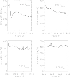
Figure 6. Lyα line widths as a function of time for the four times that Comet Lovejoy crossed the UVCS slit. The line widths have not been corrected for the instrumental width, which for the 100 μm slit used is about 140 km s−1. We estimate the systematic uncertainty to be about 50 km s−1.
Download figure:
Standard image High-resolution imageTable 3 shows the values of density, solar wind speed, and the components of the velocity along a radial vector and along the LOS at the positions where the UVCS observed the comet. Figures 7 and 8 show the magnetic field lines on which those points lie and the density structure of the corona. It is apparent that during the 10 R☉ observation, the model predicts that the comet was in the fast wind, the 2 R☉ point in a closed field region, and the other three points in closed field or slow wind regions. We will compare the predictions with the observations in Section 7.1.
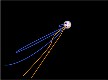
Figure 7. Magnetic field lines encountered when the comet crossed the UVCS slit as predicted by the MAS code. Each small sphere indicates the position of a comet crossing. Blue field lines are closed and orange field lines are open.
Download figure:
Standard image High-resolution image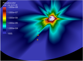
Figure 8. Densities encountered where the comet crossed the UVCS slit as predicted by the MAS code. This is a slice through the model with a viewing geometry perpendicular to the orbital plane.
Download figure:
Standard image High-resolution imageTable 3. Predicted and Observed Solar Wind Parameters
| R | nMAS | nUVCS | TMAS | TUVCS | B | Vwind | VLOS | VUVCS | θ |
|---|---|---|---|---|---|---|---|---|---|
| (R⊙) | (cm−3) | (cm−3) | (MK) | (MK) | (0.01 G) | (km s−1) | (km s−1) | (km s−1) | (°) |
| 2.10 | 1.8 × 10⁶ | 2.4 × 10⁶ | 1.43 | 1.6 | 8.37 | 2.4 | 0.15 | 0 | 54 |
| 6.36 | 2.3 × 10⁴ | 5.9 × 10⁴ | 1.15 | 0.77 | 5.71 | 223 | −99.5 | −110 | 25 |
| 8.02 | 1.7 × 10⁴ | 2.4 × 10⁴ | 1.22 | 0.47 | 4.14 | 326 | −169 | −150 | 19 |
| 10.0 | 2.3 × 10³ | 7.5 × 10³ | 1.33 | 0.36 | 2.00 | 475 | −271 | −135 | 17 |
Download table as: ASCIITypeset image
4. Analysis
In this section we present an overview of the nature of the UV emission lines and a summary of the relevant atomic rates, followed by a more detailed discussion of the Lyα intensity, velocity centroid and line width, and estimates of the outgassing rate and coronal parameters. We then turn to the lines of nitrogen, oxygen, and silicon.
4.1. Nature of the UV Emission
Hydrogen is mainly produced by photodisocciation of water, which flows from the comet at a few km s−1. The photodissociation produces H atoms with random velocities of 8–24 km s−1. These atoms form a slowly expanding spherical cloud that moves with the comet, and we refer to them as first-generation neutrals (Giordano et al. 2015). This is shown schematically in Figure 9, which indicates the different populations of neutrals from their initial production through charge transfer with coronal protons or PUIs.
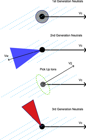
Figure 9. Schematic diagram of the distributions of first-, second-, and third-generation neutrals. The first generation is formed by photodissociation of water, the second generation by charge transfer between first-generation atoms and coronal protons, and the third generation is formed by charge transfer between first- or second-generation atoms and pickup ions. The diagram for the pickup ions indicates the ring distribution of velocity around the magnetic field direction.
Download figure:
Standard image High-resolution imageThe H atoms produce Lyα photons by collisional excitation, and they scatter Lyα photons from the solar disk. The photoexcitation tends to dominate because the Lyα emission from the disk is very bright. Because the first-generation neutrals move with the comet, the scattering is reduced by Doppler dimming (also known as the Swings effect), which becomes more severe as the comet accelerates toward the Sun. Because the first-generation cloud is fairly small due to its small expansion speed, and because it moves with the comet, it crosses the UVCS slit quickly, and it should be bright for only a few exposures. Even for smaller sungrazers than Lovejoy, the first-generation cloud is somewhat optically thick in Lyα, making it difficult to interpret the Lyα intensity without a sophisticated model.
Most of the neutral atoms undergo charge transfer with coronal protons before being ionized. There is little momentum transfer in the charge exchange process, and the resulting population of neutrals has a velocity distribution similar to that of the coronal protons. We refer to these neutrals as second-generation neutrals. They form a cloud that moves at the solar wind speed and expands with the thermal speed of the coronal protons, of order 100–150 km s−1. As the solar wind accelerates away from the Sun, Doppler dimming becomes more severe. Thus the Doppler dimming changes in the opposite sense from the behavior of the first-generation Doppler dimming as the comet moves toward the Sun, and first-generation emission is stronger far from the Sun, while second-generation emission dominates at smaller radii.
In the limit where the comet does not severely disturb the corona, each first-generation neutral that becomes ionized, whether by electron collisions, photoionization, or charge transfer, turns into a PUI (Moebius et al. 1985). The PUIs preserve their velocity component parallel to the magnetic field, while the perpendicular component initially becomes gyromotion around the field. The resulting ring beam in velocity space is highly unstable, and it quickly turns into a bispherical shell in velocity space (Williams & Zank 1994; Isenberg & Lee 1996). On a longer timescale, the PUIs scatter into a Maxwellian distribution. Oxygen PUIs show up as the striations seen in AIA images of comet Lovejoy close to the Sun (Downs et al. 2013; McCauley et al. 2013; Raymond et al. 2014). When PUI protons undergo charge transfer with either a first- or second-generation neutral, they form a population of neutrals with the PUI bulk velocity parallel to the field and quasi-isotropized gyrovelocity. These third-generation neutrals have a distinct spatial and velocity signature in UVCS observations of comet C/2002 S2 (Giordano et al. 2015), but the huge outgassing rate of comet Lovejoy may produce a bow shock at the heights of the UVCS observations, preventing the formation of a clear third-generation population.
The first-, second- and third-generation neutrals all have different sensitivities to Doppler dimming, and the interpretation of the observations in terms of outgassing rate and coronal density depends on which population dominates the emission. The three populations produce different velocity signatures, so we can attempt to sort them out.
The emission in the N, O, and Si lines is also produced by a combination of collisional excitation and photoexcitation, but the balance is different than for Lyα for several reasons. The disk emission is much fainter in these lines, and they have smaller velocity widths, so Doppler dimming is more severe. Moreover, the O v] intercombination line has a very small scattering cross section. Thus the collisional excitation component is relatively much stronger than in the case of Lyα. Another consideration is that it takes a relatively long time for atoms to be ionized up to and through the observed ionization states compared to the ionization time of hydrogen (see Section 4.2).
The N, O, and Si lines arise from ions, which cannot cross the magnetic field. They can become PUIs, as discussed above, or they may be confined to a magnetically isolated ion tail. An ion tail is in fact visible in the LASCO images, for instance in the C3 images around 22:00 UT on December 15. We will use the observed Doppler shifts to estimate the velocities, and hence the Doppler dimming, that affects the emission from these ions.
The oxygen and nitrogen arise from volatiles, while the silicon arises from sublimation of dust grains. In the 2–10 R☉ range considered here, solar radiation heats the grains to such high temperatures that vaporization dominates over collisional sputtering. The sublimation time for 1 μm grains changes drastically over this range of heights, from about 1 s at 2 R☉ to hours at 10 R☉, depending on the particular silicate mineral (Kimura et al. 2002). This is apparent from the disappearance of the bright tail seen in LASCO images as the comet approaches the Sun (Sekanina & Chodas 2012). Thus we expect the Si iii line to reveal essentially all the silicon from the evaporating comet at 2 R☉, while at 10 R☉ we see a fraction of the silicon coming off the comet, and we see silicon from the long dust tail as it crosses the slit.
4.2. Atomic Processes
Only a few atomic processes govern the observed emission lines, though their interplay is complex. We summarize them in turn, then give the number of photons produced by each atom in the observed line as it is ionized through the particular ionization stage.
Charge transfer, qct. A hydrogen atom produced by photodissociation can experience charge transfer, giving up its electron to a passing proton. This is a resonant process, so the cross section is large and strongly forward peaked (Schultz et al. 2008). Thus most of the H atoms from the comet undergo this process, and the newly formed neutrals have a velocity distribution similar to that of the coronal protons. The charge transfer rate is high because the velocity that enters is the relative speed of the comet with respect to the ambient plasma.
Collisional ionization, qion. Ionization by electron impact is somewhat slower than charge transfer. Under ionization equilibrium conditions it is balanced by recombination, but here we are looking at ions normally found at temperatures far below the temperature of the corona. Thus each ion spends a time 1/ in the ionization state observed. At a temperature of 106.2 K, the values of qion for H i, Si iii, N v, and O v are 2.88 × 10⁻⁸, 1.12 × 10⁻⁸, 1.30 × 10⁻⁹, and 2.03 × 10⁻⁹ cm3 s−1, respectively (Scholz & Walters 1991; Dere 2007). Photoionization and ionization by proton impact are slow in comparison.
Collisional excitation, qcoll. The ions are also excited by electron impact, typically at rates much higher than the ionization rate, though the intercombination line O v] has a relatively small excitation rate and Si iii has a relatively high ionization rate. We use Scholz & Walters (1991) for Lyα, and rates from CHIANTI version 7 (Landi et al. 2012) for the other lines.
Photoexcitation, qrad. Photons from the solar disk can scatter off cometary atoms or ions into our LOS. The scattering cross section is proportional to the oscillator strength of the transition, and we adopt the solar Lyα flux from TIMED/SEE (Woods et al. 2005). For Si iii and N v we scale the fluxes of Vernazza & Reeves (1978) by a factor of 1.31 to account for the higher level of solar activity indicated by the Lyα flux. The O v] intercombination line has a very small oscillator strength, so photoexcitation of that line is negligible.
The photoexcitation is complicated because it depends on the Doppler shift relative to the Sun and on the line width (Doppler dimming). Both the shift and width can change drastically over time even at a single height. In the following analysis we use the measurements shown in Figures 5 and 6, along with the comet trajectory, to determine the ratio of radial to LOS velocity. We use the Si iii and N v line widths measured at 2 R☉ to compute the rates of photoexcitation. The direction of motion of the Si iii and N v ions is determined by the local magnetic field, and we use the field structure from the MAS model described above to relate the observed Doppler shift to the Sunward component of velocity needed for the Doppler dimming calculation. The dilution of the solar radiation is determined by the distance from the Sun.
Photoionization, qphoto. Photoionization contributes only 2% to the H i ionization rate at 2.1 R☉, but that increases to 15% at 10 R☉ because the density falls off more rapidly with distance than does the radiation field. We scale the photoionization rate computed by Raymond et al. (1998) with the dilution factor and a factor of 1.3 due to the increased level solar activity. The photoionization rates for the other species can be neglected.
Photons/atom. It takes a time 1/( ) for an atom or ion to be ionized, where the collisional term is proportional to the electron density. During that time it is excited at a rate (
 ). Thus, the atom or ion produces
photons before it is ionized. Because the Lyα absorption profile is complicated by the presence of a bow shock, the Doppler dimming that determines qrad varies with time at each height. We use the measured Doppler shift and the angle between the LOS and the radial vector from the comet to the Sun to estimate radial velocity and the measured line width to determine the Doppler dimming for each exposure. The Si iii, N v, and O v] lines appear later because of their finite ionization time and, because they are relatively faint, we sum several exposures after the comet crossed the slit. We adopt the densities from the MAS model and later show that the model densities are consistent with the observations.
Table 4 shows the number of photons per atom at 2 R☉, assuming a density of  . For Lyα we determined a radial velocity of 179 km s−1. At the larger heights, the number of Lyα photons per H atom varies as the line width and centroid change, but it is typically on the order of 0.1 to 1. The numbers of photons per atom for the other lines are similar to the values at 2 R☉, but it should be kept in mind that the ionization times are longer than the times that UVCS spent at each of the upper heights, so not all the photons are captured.
Table 4. Photons per Atom at Log T = 6.2
| Line |

|

|
qrad | Nphotons |
|---|---|---|---|---|
| Lyα | 0.0518 | 0.0551 | 1.17 | 21.7 |
| Si iii | 0.0387 | 0.264 | 0.077 | 8.8 |
| N v | 0.00127 | 0.00431 | 0.001 | 38.7 |
| O v] | 0.00217 | 0.00151 | 0 | 0.69 |
Download table as: ASCIITypeset image
4.3. Bow Shock
As a comet moves through the solar wind or corona, the material it produces becomes trapped on the magnetic field lines along with the ambient plasma, and the resulting mass loading accelerates the ambient material toward the comet velocity. If the outgassing rate is high and the speed of the comet relative to the coronal gas exceeds the fast mode speed, a bow shock can form (Gombosi et al. 1996; Jia et al. 2014). The outgassing rate of Comet Lovejoy is enormous, but the Alfvén speed in the corona can exceed even the free-fall speed near the Sun, so it is not obvious whether or not a bow shock will form. While a bow shock offers a plausible interpretation for the variations in intensity, LOS velocity, and line width of Lyα at the upper three heights (see below), we have basically just one exposure at 2 R☉, and therefore little information. At that height the comet is moving at 450 km s−1, while the fast mode speed according to the MAS model is only 190 km s−1. However, the observed centroid shift of 105 km s−1 corresponds to a speed of only 125 km s−1 when the angle between the comet trajectory and the LOS is taken into account. Thus the existence of a bow shock at 2.1 R☉ is not established.
At the nose of a bow shock, the plasma is compressed and heated, and the bulk velocity equals the comet velocity. At 2.1 R☉, the plasma at the tip of the bow shock should be compressed and heated by about a factor of 2 for the known comet speed and fast mode speed. In the wings, the compression and heating are smaller, and the plasma has velocity components both along and perpendicular to the comet trajectory. The Lyα emission from such a structure is complicated because charge transfer takes place both in the shocked plasma and outside the bow shock, and the temperature and speed depend on distance from the comet as mass loading gradually affects the flow (Gombosi et al. 1996).
One measure of the importance of a bow shock is the standoff distance from the comet nucleus given by equating the ram pressure of the coronal gas,  where Vrel is the the dot product of Vcom and Vwind, and the ram pressure of the cometary gas
  ). This is 700, 1700, 4300, and 11,000 km at 2.1, 6.36, 8, and 10 R☉, respectively. The standoff distance can be compared with the distance that a first-generation neutral travels before a charge transfer event,
  . Note that this distance is smaller than the classical mean free path by a factor
  because the speed of the ambient gas streaming past the comet determines the charge transfer rate. The ratio of charge transfer length scale to standoff distance is around 0.1 at 2.1 R☉, about 1 at 6.36 and 8 R☉, and about 10 at 10 R☉. Thus the bow shock should strongly affect the Lyα emission at all but the 10 R☉ crossing.
5. Interpretation of Lyα
We first consider the Lyα emission, since that line is the brightest and gives the most detailed diagnostic information about the comet outgassing rate and the interaction with the solar wind and corona.
5.1. Lyα Intensities
Figure 4 shows the observed Lyα intensity in  . At the upper heights there is a sharp rise to a narrow peak followed by a more gradual decline. At 2.1 R☉, the hydrogen is so rapidly ionized that Lyα is bright for just one exposure, with fainter emission during the exposures before and after. The coronal background level of about
  in a 168'' segment of the 100 μm (28'') wide UVCS slit is normal for 2.1 R☉.
The emission before the steep rise originates in the hydrogen cloud that expands from the nucleus, providing some emission before the nucleus itself reaches the slit. After the peak, most of the emission is from neutrals that have undergone charge transfer, so they share the velocity distribution of the coronal plasma. In previous UVCS observations of sungrazing comets, the nuclei were small enough that it was possible to treat the neutral hydrogen they produced as test particles, and the decay time could be identified with the ionization timescale (Raymond et al. 1998; Uzzo et al. 2001; Bemporad et al. 2005). However, Comet Lovejoy produced far more water, and it severely disturbed the ambient medium. It probably created a bow shock at the larger heights, so that the velocity and temperature varied strongly with position in the region near the comet. The primary emission mechanism for Lyα is scattering of Lyα photons from the solar disk, which is sensitive to Doppler dimming (Noci et al. 1987). The chromospheric Lyα emission profile is about 200 km s−1 wide. The radial component of the solar wind speed is predicted to be 475 km s−1 for the 9.98 R☉ crossing (Section 3), while the radial component of the comet speed is 129 km s−1 at that height (Table 1). Therefore, the wind is quite faint, while hydrogen at the comet speed, either directly produced by photodissociation of water or in the stagnation region near the tip of the bow shock, is less severely Doppler dimmed. Thus, after the comet passes and the speed gradually returns to the undisturbed solar wind speed, Doppler dimming becomes more severe, and the intensity decline depends upon both the ionization rate and the rate of change of Doppler dimming.
5.2. Lyα Velocity Centroids
Figure 5 shows the observed velocity centroids at the same four heights. Negative values indicate velocity toward the Earth, while positive means away from the Earth. As mentioned above, the absolute velocity scale is somewhat uncertain, but the relative values should be reliable.
The variations in velocity make qualitative sense. Initially the emission seen upstream of the comet comes from a mixture of atoms moving at the solar wind speed and atoms moving with the comet. The actual situation is more complicated, in that when neutrals are ionized they mass load the wind, slowing it down in the comet frame. When the comet reaches the slit, the emission is dominated by atoms at the comet speed, and afterwards the average speed shifts back toward the solar wind speed. Thus at 9.98 R☉, the first velocity measured is about −70 km s−1, intermediate between the projected wind speed of −200 km s−1 and the projected comet speed of 140 km s−1. Ten to twenty minutes later, when atoms near the comet speed dominate, the measured speed is +75 km s−1, and as time goes on the speed declines to near −150 km s−1.
We note, however, that in a broad hydrogen atom velocity distribution, those atoms at small absolute radial velocities scatter more photons than those at high velocities, creating a bias in the velocity centroid toward low absolute velocities. This has little effect for phase angles near 90°, but it becomes more severe for smaller phase angles. For the orbit of comet Lovejoy, the phase angle decreases toward the upper heights. A simple estimate of the importance of this effect can be obtained by multiplying the chromospheric Lyα profile by a Gaussian with a shift of the outflow speed and the width of the Lyα profile. For phase angles around 60° like those of the upper heights observed by UVCS, line widths of around 250 km s−1 and outflow speeds of around 250 km s−1, the LOS velocity is about 1/3 of the outflow speed, due to both the purely geometrical cos(ϕ) factor and the additional bias toward lower absolute velocities due to the overlap between the emission and absorption profiles. The effect is somewhat less severe for the 2 R☉ crossing because of the higher line width. At the most extreme values of the Doppler shift, the contribution of collisional excitation becomes relatively more important.
5.3. Lyα Velocity Widths
Figure 6 shows the observed velocity widths at the four heights. The line width is complicated because different components can contribute to the emission. Using the 9.98 R☉ widths as an example, the broad widths in the first exposures result from the summation of photons from H atoms from the comet that have penetrated upstream without interaction (positive LOS speeds) and photons from neutrals moving with the wind after charge transfer (negative LOS speeds). When the comet reaches the slit, the component of cool atoms moving with the comet dominates, and the line width drops to roughly the instrumental width. After the comet has passed, a mixture of the two components, along with emission from H atoms formed by charge transfer in the bow shock, produces a large line width once more. At still later times, the line width declines to that of the solar wind.
As with the velocity measurements, the stronger illumination of the H atoms at lower absolute radial velocities and weak illumination of the faster atoms biases the line width toward smaller values. As with the interpretation of the velocity centroids, it is difficult to estimate the magnitude of this effect from the observations themselves.
5.4. Outgassing Rates
To determine the outgassing rates, we use the Doppler dimming determined from the Lyα velocity shifts and widths and the measured intensities for each exposure to determine the number of H atoms in the UVCS field of view for each exposure. For the upper heights, we take the first exposure after the intensity settled into an exponential decay and use that decay rate with the time since the comet crossed the slit to estimate  . We include a factor of about 2 to account for the H atoms that are ionized before they can become second-generation neutrals. Table 5 shows the outgassing rates for H at each height. From the outgassing rate we can determine the effective diameter of the comet nucleus by assuming that all the energy of solar radiation falling on the sunward surface of the comet goes into vaporizing ice. These estimates are also shown in Table 5, but they are not consistent. We believe that the 2.1 R☉ estimate is most reliable, because the line width is larger than the velocity shift, making the number of photons per atom less sensitive to the details of the Doppler dimming. The estimates at the larger heights are more sensitive to the velocity centroid, which as mentioned earlier is uncertain due to the degradation of the UVCS detector and to the factor used to convert the observed LOS velocity to the radial velocity that determines Doppler dimming.
Table 5. Outgassing Rate and Effective Diameter
| R |

|
Diameter |
|---|---|---|
| (R⊙) | (s−1) | (m) |
| 2.10 | 2.0 × 1031 | 220 |
| 6.36 | 1.0 × 1030 | 180 |
| 8.02 | 2.0 × 1030 | 334 |
| 10.0 | 3.6 × 1030 | 540 |
Download table as: ASCIITypeset image
5.5. Coronal Density
In previous studies of sungrazing comets we were able to assume that the comet did not disturb the coronal gas and that a single number characterized the number of Lyα photons per second scattered by each generation of neutrals. In the case of comet Lovejoy, the large variations in Lyα centroid and line width at all but the lowest height show that the corona is strongly perturbed and that the decline in intensity is at least partly due to changes in Doppler dimming. We attempt to correct for the latter effect by using the line centroid and width for each exposure to compute the Doppler dimming factor and the corresponding number of H atoms for each exposure. The comet's orbit is used to infer the radial velocity of the first-generation gas from the observed LOS velocity, and the Doppler dimming factors are computed with a code provided by S. Cranmer (2008, private communication).
At the larger heights, the derived hydrogen densities drop rapidly at first, probably because the coronal gas is compressed by the bow shock and because the cometary gas itself increases the density, but also because the effect of Doppler dimming becomes more severe as the hydrogen cloud approaches the solar wind velocity. About half way through the exposure sequence at each of the three larger heights, the intensity decline settles into an exponential decay, and we use the timescales of those decays and the ionization rates from Section 4.2 to estimate the densities. These are shown in Table 3 along with those predicted by the MAS MHD model.
6. Interpretation of Si iii, N v, and O v] Lines
Si iii, N v, and O v ions are the other products of comet outgassing that are observed in the UVCS band. The major differences from H i emission are that the Si must be liberated from dust grains and that the timescales for ionization to and through the N v and O v ionization states are relatively long.
The lifetime of a 1 μm grain at 2 R☉ is of order 1 s because the equilibrium temperature exceeds 2000 K (Kimura et al. 2002). Therefore, the sublimation time makes little difference. However, at 10 R☉, it ranges from hundreds of seconds to many hours, depending upon minerals that make up the grains, so the Si iii emission comes from silicates sublimated from dust in the tail and dissociated. Moreover, the ionization time of Si iii at the low density at 10 R☉ is hours. Figure 10 shows the intensities of Si iii λ1205 and Lyα as a function of time for the 9.98 R☉ crossing, and the difference between Si iii and Lyα is readily apparent.
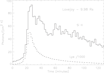
Figure 10. Temporal behavior of Si iii emission at 10 R☉ with scaled Lyα emission shown for comparison. The Si iii emission persists much longer than the Lyα, because it arises from dust in the comet's tail as it evaporates and because of the long ionization timescale.
Download figure:
Standard image High-resolution imageThe ionization timescales to reach N v and to pass through it are 3.8 × 10⁸/ne and 7.6 × 10⁸/ne s, respectively, assuming log T = 6.2. For an assumed density of  at 2.1 R☉ (see below), we would expect N v emission to extend from about 200 to 600 s after the comet passes. Figure 11 shows the N v emission for the 2.1 R☉ crossing. The observed flux peaks at about 370 s after the comet passes through the slit, which agrees well with the predicted ionization times.

Figure 11. N v λ1238 flux at 2.0 R☉ as a function of time. The average of the first nine exposures has been subtracted as coronal background, and the exposure where Lyα peaks is indicated by the dashed lines.
Download figure:
Standard image High-resolution image
6.1. Si iii and N v Line Widths
As discussed above, the Lyα line width varies from exposure to exposure. The Si iii and N v lines are fainter, so we consider the 2.1 R☉ crossing and sum the seven exposures brightest in N v to measure the line width. Gaussian fits give widths of 205 and 181 km s−1 (FWHM) for Si iii and N v, respectively. That suggests that when Si and N atoms are released from the comet and ionized, a substantial fraction of the comet's speed becomes gyro motion about the magnetic field. From the comet's trajectory and the magnetic field orientation predicted by the MHD model discussed below, we expect that 384 km s−1 of the comet speed will become gyro motion. That should isotropize to some extent to form a bispherical distribution (Williams & Zank 1994; McCauley et al. 2013) with a line width of order 240 km s−1. Some of the energy is lost to generation of Alfvén waves, and Coulomb collisions with protons will slow the Si2+ and  ions on timescales of 2280 and 290 s, respectively (Downs et al. 2013), so collisions will have little effect on the Si ions during their ionization time, but will slow the N ions significantly. Overall, the line widths are consistent with the predictions, though a larger difference between the Si iii and N v lines due to Coulomb collisions might have been expected.
6.2. Elemental Abundances
From the intensities of the H i, N v, O v], and Si iii lines and the numbers of photons per atom listed in Table 4, we can determine the relative abundances of H, N, O, and Si. We use the crossing at 2.1 R☉ because the O v] line is not detectable at the larger heights, the ionization timescale for N is large at the larger heights, and Si is liberated from grains rapidly at 2.1 R☉ but slowly at the larger heights.
During the 2.1 R☉ crossing, the H i and Si iii lines only appeared in three exposures, 23:33:24 to 23:39:32 UT, while the N v and O v] lines peaked several exposures later and faded away toward the end of the observing sequence. We sum the H i and Si iii photon fluxes observed during the three peak exposures and the N v and O v] fluxes from 23:39:36 UT to 00:16:44 UT to obtain relative fluxes in the Lyα, N v, O v], and Si iii lines of 1:0.0095:0.024:0.070. We divide by the numbers of photons per atom in Table 4 to obtain H: N: O: Si abundance ratios (by number) of 1:0.005:0.86:0.18.
The oxygen abundance would be 0.5 if the H and O arose from H2O, and it would be higher if SiO2 contributed significant oxygen. We can estimate the SiO2 contribution if we assume that all the Si detected by UVCS comes from SiO2, or at least from minerals with about the same ratio of Si to O. The Si:H ratio of 0.18 given above implies an O:H ratio of 0.86, in remarkable agreement with the derived O abundance. However, that must be fortuitous, because the O v] fluxes are very difficult to measure due to blending with Lyα, and we estimate the uncertainty to be a factor of 1.5.
7. Discussion and Comparison with Other Work
7.1. Comparison of Coronal Parameters with MAS Model Predictions
The coronal densities determined from UVCS are compared with those from the MAS model in Table 3. The densities from the UVCS range from 1.3 times the MAS density at 2.1 R☉ to three times the MAS density at 10 R☉. This could be a result of the bias in the velocity measurements that would lead to an underestimate of the severity of Doppler dimming, which would become a larger factor at larger heights. It is apparent from Figure 8 that the comet positions at the upper heights lie on fairly steep density gradients. Therefore, a small shift in longitude, as was suggested by comparison of the magnetic field directions inferred from AIA with the MAS model (Raymond et al. 2014), might account for the differences between the UVCS and MAS densities. However, with the exception of the 10 R☉ crossing the differences probably lie within the uncertainties of the UVCS determinations due to the systematic uncertainty in the velocity centroids and the approximate treatment of the Doppler dimming.
Table 3 also compares the LOS components of the solar wind velocity predicted by the MAS model with the Doppler shifts measured by the UVCS. At 2.1, 6.4 and 8 R☉, the agreement is quite good. At 10 R☉ the velocities differ by a factor of 2. A shift in longitude that gave a higher predicted density would give a lower predicted VLOS, in agreement with Table 3, so that explanation is consistent with both the density and velocity comparisons. However, the bias toward lower velocities due to the overlap of the absorption profile with the disk emission profile discussed in Section 4.2 is most severe at 10 R☉ both because of the higher wind speed and the lower phase angle, so that is also likely to play a role.
Table 3 also lists the temperatures predicted by the MAS model and determined from the UVCS line widths long after the comet's passage. From Figure 6, it is clear that the line width at 2.1 R☉ is well determined, and those at the other heights seem to be approaching constant values. However, the systematic uncertainty in the line width due to the detector degradation could be quite significant. It would affect the narrower lines more strongly than the wider lines. For instance, if the line widths were underestimated by our estimated uncertainty of 50 km s−1 at the 10 and 8 R☉ crossings, the temperatures would be increased to 0.64 and 0.77 MK. These values are still below the MAS predictions, but are not unreasonable in comparison with typical temperatures measured at 1 au. Overall, the agreement for the most reliable measurement is encouraging, but the derived temperatures at the upper heights are probably underestimates.
Of course another possibility is that the solar wind densities are simply underestimated in the MAS model and/or flow speeds are overestimated. This may occur if the model solar wind is accelerated too much or too quickly in this region of the inner heliosphere. More sophisticated models of the fast solar wind include treatments for wave reflection and/or dissipation (e.g., Cranmer et al. 2007; Verdini & Velli 2007; Chandran & Hollweg 2009), and these treatments influence the hydrodynamic profiles as a function of distance. Such techniques are beginning to make their way into multi-dimensional MHD models (Usmanov et al. 2012; Lionello et al. 2014; van der Holst et al. 2014), and to be tested by sensitive plasma diagnostics, such as frozen in charge states (e.g., Landi et al. 2014). This suggests that such single-point estimations of plasma conditions as a function of distance (as provided by Comet Lovejoy), while subject to measurement uncertainty, may be useful in constraining solar wind models in the future.
We should also mention that this MAS run used a single-fluid approximation for electrons and protons in the MHD calculation. Extending the model to use a multi-fluid or multi-temperature treatment with variable partitioning of heat between protons and electrons would also influence the modeled temperature of the proton population as a function of height.
7.2. Grain Sublimation Rates in the Tail
The UV spectra show strong Si iii emission well after the comet passes through the UVCS slit, and it probably arises from sublimation of silicate grains in the comet tail. If so, the combination of LASCO and UVCS data provides the possibility of measuring the sublimation rates of dust grains at the high temperatures expected close to the Sun. From the visible light brightness, an assumed albedo, and an assumed fraction of the brightness due to dust scattering, we find the total area of dust grains within the UVCS aperture listed in Table 2. The production rates of silicon are determined from the Si iii intensities and the number of photons per atom. The ratio of these numbers, along with an assumed density of  , gives the sublimation rate in cm s−1, and we use that to determine the sublimation times for a 0.2 μm grain listed in Table 2.
Kimura et al. (2002) give theoretical predictions for the lifetimes of 0.2 μm silicate grains. They consider both amorphous and crystalline olivines and pyroxenes, but the crystallization times for both minerals are under 10 s at the heliocentric distances observed here, so we only consider the crystalline forms. Figure 4 of Kimura et al. (2002) gives sublimation times for olivines of about 2 and 300 s at 8 and 10 R☉, respectively, which are smaller than the timescales in Table 2 and the roughly 2 hr timescale for the fading of Si iii emission at 10 R☉ seen in Figure 10. On the other hand, Figure 4 of Kimura et al. (2002) shows sublimation times for crystalline pyroxenes exceeding 104 s at heliocentric distances above 5.5 R☉. Thus at first glance, neither mineral matches the observations. On the most basic level, the similarity, or even modest increase, of τ0.2 between 10 and 8 R☉ does not match expectations of more rapid sublimation as the grains get closer to the Sun. However, the drastic drop in sublimation time between 8 and 6.36 R☉ is similar to the steep curves in the Kimura et al. (2002) sublimation times.
There are several major caveats to this comparison. On the observational side, there is a delay between the grain sublimation and the observation of Si iii emission due to the ionization time. While this is only a few seconds at 2 R☉, it is on the order of half an hour at the upper heights. In general, taking this delay into account would roughly double the sublimation timescales. We have also assumed an albedo of 0.04, but it could be up to 10 times larger. That would mean a smaller total dust area and a larger sublimation rate. It is also important to note that LASCO C2 images with the orange filter give larger grain surface areas than those we derived from the C3 images (Section 2.2). The C2 values would give sublimation times an order of magnitude larger than those in Table 2, but still smaller than the lifetimes at larger heights, and intermediate between the Kimura et al. (2002) predictions for olivines and pyroxenes. A potentially fundamental problem is that the Si iii might reside in an ion tail rather than the dust tail. Such an ion tail is visible in some LASCO images, but we have no means to quantify its elemental or ionic composition. Another potential complication is that after the comet passes through the slit, the dust in the tail at later times no longer lies along the orbit, but at larger distances. That would tend to increase the lifetime.
On the theoretical side, Kimura et al. (2002) assume that the grains are aggregates of smaller (70, 100, or 150 nm) particles of pure olivine or pyroxene composition. Their calculations show that the olivine grains are about 200 K hotter than the blackbody temperature at 12 R☉, while the pyroxene grains are about 300 K cooler than the blackbody temperature. The sensitivity of the sublimation rate to the grain temperature presumably accounts for the great differences in sublimation times. If the grains were aggregates of both olivines and pyroxenes, they would presumably have an intermediate temperature and sublimation time, and that would be in line with our observations. Furthermore, Kimura et al. (2002) show that the equilibrium grain temperature peaks at sizes around 0.2 μm, and olivine grains of that size sublimate rapidly at around 11 R☉, in agreement with LASCO observations. On the other hand 1 μm grains are a few hundred K cooler and sublimate far more slowly. The sublimation rate depends exponentially on the temperature, and a distribution of grain sizes could give a broad distribution of lifetimes. A properly chosen distribution of olivine grains might be able to match both the fading observed at 11–12 R☉ (Biesecker et al. 2002; Knight et al. 2010) and the lifetimes that we obtain at smaller heights.
7.3. Nucleus Diameter
The diameter of the nucleus should shrink by tens of meters as it approaches from 10 R☉ and passes through perihelion. We estimate the diameters at four heights during ingress and compare them with those estimated from other observations at earlier and later times. The size of the nucleus can also be estimated from the outgassing rate with the assumption that all the energy of the sunlight absorbed by the nucleus goes into sublimating ice. The albedo is generally taken to be small, and we assume 0.04. Equation (4) of Bemporad et al. (2005) gives the effective area of the nucleus, which implies an effective diameter if it is spherical. Table 5 gives the diameters obtained with this method. Aside from uncertainty in the outgassing rate, there are two other concerns about this approach. If the comet fragments, the absorbing area becomes much larger, and the diameter will be overestimated. On the other hand, if the coma blocks a large fraction of the light that would otherwise strike the comet, the diameter will be underestimated. It is also possible that the dark crust of the comet is blown off by high pressures under the surface as the comet heats up during the approach to perihelion, and that could expose a surface with higher albedo, again leading to an underestimate of the diameter.
There are a few other estimates for the size of Comet Lovejoy. Gundlach et al. (2012) estimated a diameter of 1 km at 12 R☉ by comparing the visual brightness with those of other sungrazers at that heliocentric distance. McCauley et al. (2013) used the total amount of oxygen lost during the egress observation of Comet Lovejoy by AIA to estimate a diameter of 363 m. There were outbursts during the AIA observations, quite likely corresponding to increases in the effective surface area due to fragmentation, and the 363 m estimate comes from a time when it was relatively bright (McCauley et al. 2013). Sekanina & Chodas (2012) estimated a diameter of 150–200 m when the comet disintegrated 1.6 days after perihelion. We can also obtain an estimate by using the outgassing rate of 1032.5 s−1 measured by McCauley et al. (2013) early in the egress and Equation (4) of Bemporad et al. (2005). That leads to a diameter of 500 m, but the outgassing rate corresponds to a brightness peak and probably results from some fragmentation, so the average diameter would be smaller.
Our diameter estimates of 540 and 334 m at the upper two heights are compatible with the diameters estimated during egress and at breakup, but the diameters near 200 m obtained for the 2.1 and 6.36 R☉ crossings seem to be too small. That suggests that we have underestimated the outgassing rates at these heights or that the coma shields the nucleus from solar radiation. The optical depth of the Lyα cloud is likely to be the problem at 2.1 R☉. Even the cloud of second-generation neutrals should have an optical depth of order unity in Lyα at the radius of a few times 109 cm where ionization becomes important. That will reduce the number of photons scattered by each atom and lead to an underestimate of the outgassing rate and the nucleus diameter. It would also lead to an underestimate of the ratios of H to N, O and Si.
7.4. Elemental Abundances
McCauley et al. (2013) used AIA observations of Comet Lovejoy shortly after perihelion to estimate the elemental abundance ratios C:O = 0.006 and Fe:O = 0.05. Combining these with the the estimates from Section 6.4, we find H:C:N:O:Si:Fe = 1:0.005:0.005:0.86:0.18:0.04. The very low abundances of C and N suggest that a only a small fraction of the volatile elements were incorporated into the comet during formation or that volatiles had been lost during previous perihelion passages or during the approach to perihelion.
Two other sungrazers show Si iii emission in UVCS spectra. Ciaravella et al. (2010) observed comet C/2003 K7 at 3.37 R☉. A re-examination of the spectra indicates that the blend of C iii and Si iii lines is dominated by Si iii, in which case the Si:H ratio is about 0.04. Bemporad et al. (2005) used the UVCS spectra of comet C/2001 C2 at 4.98 R☉ to estimate Si:H ∼0.05. Both these values are below the ratio Si:H = 0.18 derived above from our observation at 2.1 R☉. For the density derived by Bemporad et al. (2005) from the decay of the Lyα intensities, the Si iii ionization time for comet C/2001 C2 is 3000 s, so about half of the Si emission would have been missed in the 2200 s UVCS observation after the slit crossing, and the Si:H ratio should be increased to at least 0.10. The density is not well determined for comet C/2003 K7. The UVCS observation lasted only 700 s, but the ionization time is expected to be around 100 s for typical streamer densities at 3.4 R☉. However, for fast wind densities a significant amount of Si emission might have been missed. Overall, we think that the higher Si abundance estimated for Comet Lovejoy is more reliable, but it is also possible that the dust-to-gas ratio differs among the Kreutz comets.
Comet Lovejoy may be different from the previously observed Kreutz comets due to their different sizes. Ground-based observational evidence suggests (e.g., Ye et al. 2014) that the small Kreutz comets are not active far from the Sun, perhaps because they are depleted of accessible volatiles (H2O, CO, CO2). Lovejoy was observed as an active comet at those distances. Thus, the small sungrazers may not be releasing Si-bearing grains into a tail until nearly at the Sun, while Lovejoy had already produced a substantial population of grains. Thus, the small comets may be more indicative of the bulk Kreutz composition since everything is being produced essentially instantaneously, while Lovejoy may be biased by older, larger grains remaining near the nucleus. On the other hand, it is possible that the small comets had lost volatiles and are less representative.
8. Summary
We observed the sungrazing Comet C/2011 W3 (Lovejoy) with the UVCS spectrometer and the LASCO coronagraph. We obtained local (as opposed to LOS-averaged) estimates of the coronal density, temperature, and outflow speed at four points where the comet crossed the UVCS slit. The observations are in qualitative agreement with our understanding of the interaction between the comet and the corona and with coronal plasma parameters predicted by the MAS MHD code (Downs et al. 2013), but our estimates are uncertain at the 30% to factor of 2 level.
We also estimated the size, outgassing rate, and elemental composition of the comet. The size and composition are compatible with other estimates, again at the factor of 2 level. Finally, we estimated the sublimation rate of silicate grains by comparing the white light intensity from LASCO with the Si iii intensity from UVCS. There are many uncertainties in this comparison, but the rates are very different from those of either 0.2 μm olivine or pyroxene grains predicted by Kimura et al. (2002), although they are compatible with a mixture of the two minerals or a range of grain sizes.
Unlike the low corona, where EUV observations provide reasonable constraints on the simulated density and temperature distributions, it remains challenging to observationally vet such models in the extended corona (2–20 R☉) where a good fraction of the solar wind heating and acceleration takes place. Because each sungrazing comet effectively samples the corona at a series of points, rather than giving integrated values along the LOS, these comets offer a unique opportunity to test our hydrodynamic prescriptions for the solar wind. The dramatic changes in Lyα intensity, velocity centroid, and line width show that the comet strongly affects the corona at the larger heights observed, presumably by way of a bow shock. More detailed analysis of those changes will require an MHD model that incorporates a separate neutral population, along the lines of the models of Gombosi et al. (1996) and Jia et al. (2014).
Some of this work was begun at the workshop "The Science of Near-Sun Comets" led by G. Jones at the International Space Science Institute (ISSI) in Bern, Switzerland in 2014–2015. M.K. was supported by NASA Outer Planets Research grant NNX13AL02G. K.B. was supported by the NASA Sungrazer Project, NASA grant NNG12PP90I. We thank G. Jones for helpful comments.
Facility: SOHO - Solar Heliospheric Observatory satellite (UVCS, LASCO).