


Abstract
We report on ephemerides for the satellites of Pluto based on the large set of astrometric measurements. Our orbit fit yielded the following masses with 1σ uncertainties: GMPluto = 869.3 ± 0.4 km3 s−2, GMCharon = 106.1 ± 0.3 km3 s−2, GMNix = 1.50 ± 0.52 × 10⁻³ km3 s−2, GMHydra = 2.01 ± 0.27 × 10⁻³ km3 s−2, corresponding to the densities of ρPluto = 1.853 ± 0.004 g cm−3, ρCharon = 1.705 ± 0.006 g cm−3, ρNix = 0.88 ± 0.31 g cm−3, and ρHydra = 1.21 ± 0.19 g cm−3. Masses of Kerberos and Styx remain unconstrained, and it is unlikely that we will be able to measure them even if we obtain abundant 1 mas precision astrometry during the next 20 yr. We summarize the results of orbit integration in terms of osculating and precessing ellipse model mean elements. All satellites reside in near-circular orbits, and Kerberos and Styx have 0.4 deg and 0.3 deg inclinations with respect to Charon's orbit plane. The nodal regression periods for Kerberos and Hydra are ∼9 and ∼14 yr respectively. We found that Charon's orbit pole can be approximated as: R.A. = 133.0073 + 0.0036T deg, and decl. = –6.2449 + 2.5 × 10⁻⁵T deg, where T is Julian centuries from the epoch J2000, based on 5000 yr of orbit integration.
Export citation and abstract BibTeX RIS

Original content from this work may be used under the terms of the Creative Commons Attribution 4.0 licence. Any further distribution of this work must maintain attribution to the author(s) and the title of the work, journal citation and DOI.
1. Introduction
In 2015, NASA's New Horizons mission investigated the Pluto system. Stern et al. (2018) summarized what was known about the system before the mission, what was learned during the flyby, and how future exploration of the Kuiper Belt may look like. The Pluto system has five satellites: Charon, Styx, Nix, Kerberos, and Hydra. The largest satellite, Charon, orbits Pluto with ∼6.4 days period, and the pair is tidally locked. The rest of the satellites form a continuous sequence of near-resonant orbits (1:3:4:5:6) with respect to the Pluto–Charon orbital period. Pluto and Charon have a high mass ratio, ∼0.12 (Buie et al. 2006; Tholen et al. 2008; Brozović et al. 2015), and the planet is only about twice the size of Charon (1188.3 km versus 606 km radii Stern et al. 2018). The leading theory for the origin of the Pluto–Charon binary is a giant impact (McKinnon 1989; Canup 2005). The small satellites presumably formed from the leftover debris (Stern et al. 2006), and many numerical studies attempted to elucidate how the collisionally interacting debris evolved over time (Canup 2011; Youdin et al. 2012; Kenyon & Bromley 2014; Walsh & Levison 2015; Canup et al. 2021). The detailed knowledge of the satellites' masses and orbits is a prerequisite for any dynamical model, but the small satellites' astrometry was sparse and their orbits were not well constrained until recently. Weaver et al. (2006), Tholen et al. (2008), Beauvalet et al. (2013) reported on orbits and order-of-magnitude constraints on the masses of Nix and Hydra based on very limited data. Brozović et al. (2015) reported a substantial set of Hubble Space Telescope (HST) astrometry on all small satellites (including Kerberos and Styx), and their JPL's PLU043 ephemeris were used by the New Horizons Optical Navigation Team (Pelletier et al. 2016).
The latest orbit fit for all satellites except Charon was published by Porter & Canup (2023). The authors reduced an extensive set of the HST astrometry with respect to the stars in Gaia DR2 catalog (Gaia Collaboration et al. 2018), and they also reduced the astrometry obtained with the New Horizons Long Range Reconnaissance Imager (LORRI). This resulted in hundreds of measurements of Nix, Hydra, Kerberos, and Styx over more than a decade, 2005–2019. Porter & Canup (2023) fit this data with orbits numerically integrated with a high-order Runge–Kutta–Nystom adaptive time step integrator and Markov chain Monte Carlo estimation process for seven free parameters per satellite (position, velocity, and mass). The system mass and Charon's mass and orbit were not fit, but instead JPL orbit solution PLU055 (Jacobson et al. 2015) was used. Porter & Canup (2023) was the first study to show clear sensitivity for masses of Nix and Hydra (GMNix = 0.0017 ± 0.00035 km3 s−2, GMHydra = 0.0020 ± 0.0002 km3 s−2), where GM is mass multiplied by the Newtonian gravitational constant G. Masses of Kerberos and Styx remain unconstrained, but it is reasonable to assume that they have similar density, ∼1 g cm−3, as Nix and Hydra.
Our goal was to fit all satellites of Pluto simultaneously in order to keep all the masses and the barycenter location self-consistent. Fitting Charon's orbit represents the largest challenge because of the various types of measurements that start with photograpic plates from 1965 and end with Gaia absolute astrometry from 2019. The current astrometric data set is significantly larger than what was used in Brozović et al. (2015). We used all available astrometry of Nix, Hydra, Kerberos, and Styx, including some Hubble data on Nix and Hydra that were not rereduced by Porter & Canup (2023
2. Methods
2.1. Astrometric Data
Charon's astrometry is listed in Table 1. Harrington & Christy (1980) reported on position measurements of Charon with respect to Pluto that predate its discovery in 1978 (Christy & Harrington 1978). Pluto and Charon were not fully resolved in the photographic plates, but it was possible to measure the image elongation and orientation and express Charon's position relative to Pluto in terms of position-angle Δθ and separation Δρ. These early observations had measurement uncertainties of ∼150 miliarcseconds (mas). Soon after its discovery, Charon was also observed via speckle interferometry from several large telescopes around the world (Bonneau & Foy 1980; Baier et al. 1982; Hege et al. 1982; Hetterich & Weigelt 1983; Hege & Drummond 1984; Baier & Weigelt 1987; Beletic et al. 1989). In 1984 and 1985, Beletic et al. (1989) reported 56 speckle interferometric measurements of Charon's separation from Pluto in terms of R.A. projected onto a tangential plane ( ) and decl. (Δδ).
Table 1. Charon Astrometric Observations
| Time Span | Type | Points | rms | Type | Points | rms | References |
|---|---|---|---|---|---|---|---|
| (mas) | (mas) | ||||||
| 1965 Apr–1979 Apr | ρΔθ | 23 | 105 | Δρ | 12 | 146 | Harrington & Christy (1980) |
| 1980 Jun–1984 Feb | ρΔθ | 2 | 18 | Δρ | 2 | 83 | Hege et al. (1982), Hege & Drummond (1984) |
| 1980 Jun | ρΔθ | 5 | 15 | Δρ | 5 | 29 | Bonneau & Foy (1980) |
| 1981 Apr | ρΔθ | 2 | 11 | Δρ | 2 | 22 | Hetterich & Weigelt (1983) |
| 1981 Apr–1983 Jul | ρΔθ | 8 | 41 | Δρ | 8 | 82 | Baier et al. (1982), Baier & Weigelt (1987) |
| 1984 May–1985 May |

| 56 | 87 | Δδ | 56 | 73 | Beletic et al. (1989) |
| 1991 Aug–1993 Aug | Sample | 28 | 11 | Line | 28 | 15 | Null et al. (1993), Null & Owen (1996) |
| 1992 May–1993 Aug |

| 60 | 3 | Δδ | 60 | 3 | Tholen & Buie (1997), Buie et al. (2012) |
| 1992 Feb–1992 Mar |

| 80 | 30 | Δδ | 80 | 12 | Young et al. (1994) |
| 1998 Mar | α | 5 | 14 | δ | 5 | 15 | Olkin et al. (2003) |
| 2002 Jun–2003 Jun |

| 384 | 3 | Δδ | 384 | 2 | Buie et al. (2006), Buie et al. (2012) |
| 2005 May | ρΔθ | 2 | 24 | Δρ | 2 | 8 | Weaver et al. (2006) |
| 2005 Jun |

| 45 | <1 | Δδ | 45 | <1 | B. Sicardy et al. (2006, personal communication) |
| 2005 Jul | α | 1 | 4 | δ | 1 | 4 | Herald et al. (2020) |
| 2006 Apr |

| 1 | 11 | Δδ | <1 | 6 | Sicardy et al. (2006) |
| 2006 Feb |

| 10 | 3 | Δδ | 10 | 3 | Brozović et al. (2015) |
| 2007 Mar–2007 Jun |

| 215 | 3 | Δδ | 215 | 3 | Buie et al. (2012) |
| 2008 Jun |

| 1 | 1 | Δδ | 1 | <1 | Sicardy et al. (2011) |
| 2010 Apr–2010 Sep |

| 95 | 3 | Δδ | 95 | 2 | Brozović et al. (2015) |
| 2010 Apr–2010 Sep |

| 240 | 3 | Δδ | 240 | 2 | Buie et al. (2012) |
| 2011 Jun |

| 2 | <1 | Δδ | 2 | <1 | B. Sicardy et al. (2015, personal communication), |
| 2011 Jun–2011 Sep |

| 104 | 3 | Δδ | 104 | 2 | Brozović et al. (2015) |
| 2012 Jun–2012 Jul |

| 548 | 2 | Δδ | 548 | 2 | Brozović et al. (2015) |
| 2012 Jul | ρΔθ | 1 | 4 | Δρ | 1 | 1 | Howell et al. (2012) |
| 2014 Jul | Sample | 74 | 81 | Line | 74 | 105 | Pelletier et al. (2016), Thompson et al. (2016) |
| 2015 Jan–Feb | Sample | 75 | 39 | Line | 75 | 53 | Pelletier et al. (2016), Thompson et al. (2016) |
| 2015 Apr–Jul | Sample | 379 | 126 | Line | 379 | 158 | Pelletier et al. (2016), Thompson et al. (2016) |
| 2014 Sep–2019 Nov | AL | 232 | 1.4 | AC | 232 | 142 | Tanga et al. (2023) |
Note. Summary of Charon's optical astrometry. We list the time of observations, type of measurement, number of astrometry points, and the rms of the residuals. Note that Pelletier et al. (2016) and Thompson et al. (2016) are the New Horizons optical navigation data obtained as the spacecraft was approaching the system.
Download table as: ASCIITypeset image
Charon's orbit was constrained with lightcurves during the Pluto–Charon mutual event season that lasted from late 1984 until late 1990 (Tholen et al. 1987). There were 64 lightcurves reported: 15 from Palomar (Buratti et al. 1995), 39 from Maunakea Observatory (Tholen 2008), and 10 from McDonald Observatory (Young 1993; Young & Binzel 1993). These lightcurves are available on NASA Planetary Data System Small Bodies Node. 1
Null et al. (1993) and Null & Owen (1996) used the HST Wide Field Camera to measure absolute positions of Pluto and Charon as "Samples" and "Lines" in camera coordinates. The goal was to detect Pluto's barycentric motion and to estimate the individual masses and bulk densities. We used Gaia DR3 reference stars (Tanga et al. 2023) to re-point these images. Buie et al. (2012) reported more relative measurements ( and Δδ) of Charon. These HST measurements were originally obtained by Tholen & Buie (1997), but Buie et al. (2012) rereduced and corrected them for the center-of-light and center-of-body offset based on an early model for Pluto's albedo.
Young et al. (1994) used Maunakea's Observatory 2.2 m telescope on six nights in 1992 February to demonstrate that it is "... possible to perform precise astrometry of Pluto and Charon from large, ground-based telescope using PSF fitting techniques." Their observations were successful, but the ground-based astrometry remains sparse to this day. During the several decades of followup, Charon's astrometry has been predominantly obtained with the HST. Most of these measurements were relative observations (Buie et al. 2006, 2012; Weaver et al. 2006; Brozović et al. 2015), but Olkin et al. (2003) reported five absolute measurements (α, δ) that were important for early Pluto/Charon mass-ratio determination (0.122 ± 0.008).
B. Sicardy et al. (2006, personal communication) reported relative astrometry of Charon derived from adaptive optics observations (NACO/VLT at Paranal) from 2005. One more point was obtained in 2006 as Hydra was followed up from the same site (Sicardy et al. 2006). The last ground-based measurement with speckle interferometry (ρΔθ, Δρ) was obtained by Howell et al. (2012).
Stellar occultations yield high-accuracy measurements of Charon's position. Sicardy et al. (2011) reported a Pluto and Charon occultation of the same star on 2008 June 22. Two more Charon occultation points (2011 June 4 and 23) were reported by B. Sicardy via personal communication. We also used the 2005 July 11 stellar occultation reported by Herald et al. (2020).
The New Horizons Optical Navigation Team reported Charon's astrometry (Pelletier et al. 2016; Thompson et al. 2016) based on raw images that are publicly available on NASA Planetary Data System (see footnote 1) archive. There were more than five hundred measurements of the absolute position of Charon from 2014 July 19 to 2015 July 15. The close approach occurred on 2015 July 14.
The Gaia space telescope detected Charon in the instances when its location was at least 0.25 mas away from Pluto in the scan direction (AL direction; Tanga et al. 2023). We identified 31 transits with Charon observations in the Gaia FPR. 2 The data from different transits are at least 90 minutes apart and the transits span 14 separate dates from 2014 to 2019; 23 out of 31 transits occurred in 2019. Gaia astrometry is reported in bursts of 6–10 α and δ measurements that are 5 s apart. The α and δ uncertainties have values of hundreds of mas and the measurements have high correlations (>0.99999). The correlation of α and δ measurements is a result of coordinate transformation from the original (uncorrelated) AL (along the scan) and AC (across the scan) measurements (Gaia Collaboration et al. 2018). A recent press release by the Gaia project 3 stated that this is only a preliminary data reduction, and that Pluto and Charon data will get fully reduced in Gaia DR5 release.
The measurements of small satellites' positions are listed in Tables 2–5. Most of them were obtained with the HST. There were a few more measurements obtained with NACO/VLT and Magelan I Baade telescopes (Fuentes & Holman 2006; Sicardy et al. 2006). Porter & Canup (2023) reprocessed most of the HST data with respect to the stars in the Gaia DR2 catalog, and these measurements are of especially high quality. Furthermore, Porter & Canup (2023) also reduced the New Horizons LORRI 4 × 4 optical images, and reported hundreds of measurements obtained during two months prior to the closest approach. The measurements in Porter & Canup (2023) were reported relative to the JPL DE430 planetary ephemeris location of the Pluto system barycenter (Folkner et al. 2014). Utilizing the HST or New Horizons astrometry requires knowledge of spacecraft position at each observation time. The reconstructed trajectory files for the spacecraft are available from NASA's Navigation and Ancillary Information Facility website (Acton 1996).
Table 2. Nix Astrometric Observations
| Time Span | Type | Points | rms | Type | Points | rms | References |
|---|---|---|---|---|---|---|---|
| (mas) | (mas) | ||||||
| 2002–2003 |

| 11 | 17 | Δδ | 11 | 12 | Buie et al. (2006) |
| 2005 |

| 2 | 2 | Δδ | 2 | 2 | Porter & Canup (2023) |
| 2006 |

| 3 | <1 | Δδ | 3 | 2 | Porter & Canup (2023) |
| 2006 |

| 2 | 136 | Δδ | 2 | 121 | Fuentes & Holman (2006) |
| 2007 |

| 16 | 2 | Δδ | 16 | 2 | Porter & Canup (2023) |
| 2010 |

| 10 | 1 | Δδ | 10 | 2 | Porter & Canup (2023) |
| 2011 |

| 6 | 1 | Δδ | 6 | <1 | Porter & Canup (2023) |
| 2012 |

| 6 | <1 | Δδ | 6 | <1 | Porter & Canup (2023) |
| 2013 |

| 12 | <1 | Δδ | 12 | <1 | Porter & Canup (2023) |
| 2014 |

| 11 | <1 | Δδ | 11 | <1 | Porter & Canup (2023) |
| 2015 |

| 40 | <1 | Δδ | 40 | <1 | Porter & Canup (2023) |
| 2018 |

| 13 | <1 | Δδ | 13 | <1 | Porter & Canup (2023) |
| 2019 |

| 9 | <1 | Δδ | 9 | <1 | Porter & Canup (2023) |
Note. Summary of Nix's optical astrometry and fit residuals. Note that Fuentes & Holman (2006) from 2006 are ground-based observations. The rest is the HST astrometry (Porter & Canup 2023).
Download table as: ASCIITypeset image
Table 3. Hydra Astrometric Observations
| Time Span | Type | Points | rms | Type | Points | rms | References |
|---|---|---|---|---|---|---|---|
| (mas) | (mas) | ||||||
| 2002–2003 |

| 11 | 10 | Δδ | 11 | 12 | Buie et al. (2006) |
| 2005 |

| 2 | <1 | Δδ | 2 | <1 | Porter & Canup (2023) |
| 2006 |

| 1 | 32 | Δδ | 1 | 11 | Sicardy (2006, personal communication) |
| 2006 |

| 2 | 135 | Δδ | 2 | 88 | Fuentes & Holman (2006) |
| 2006 |

| 3 | <1 | Δδ | 3 | 1 | Porter & Canup (2023) |
| 2007 |

| 16 | <1 | Δδ | 16 | <1 | Porter & Canup (2023) |
| 2010 |

| 10 | <1 | Δδ | 10 | <1 | Porter & Canup (2023) |
| 2011 |

| 6 | <1 | Δδ | 6 | <1 | Porter & Canup (2023) |
| 2012 |

| 6 | <1 | Δδ | 6 | <1 | Porter & Canup (2023) |
| 2013 |

| 12 | <1 | Δδ | 12 | <1 | Porter & Canup (2023) |
| 2014 |

| 11 | <1 | Δδ | 11 | <1 | Porter & Canup (2023) |
| 2015 |

| 40 | <1 | Δδ | 40 | <1 | Porter & Canup (2023) |
| 2018 |

| 13 | <1 | Δδ | 13 | <1 | Porter & Canup (2023) |
| 2019 |

| 9 | <1 | Δδ | 13 | <1 | Porter & Canup (2023) |
Note. Summary of Hydra's optical astrometry and fit residuals. Note that Fuentes & Holman (2006) and B. Sicardy et al. (2006, personal communication) from 2006 are ground-based observations. The rest is the HST astrometry (Porter & Canup 2023).
Download table as: ASCIITypeset image
Table 4. Kerberos Astrometric Observations
| Time Span | Type | Points | rms | Type | Points | rms | References |
|---|---|---|---|---|---|---|---|
| (mas) | (mas) | ||||||
| 2005 |

| 2 | <1 | Δδ | 2 | 1 | Porter & Canup (2023) |
| 2006 |

| 3 | <1 | Δδ | 3 | <1 | Porter & Canup (2023) |
| 2010 |

| 10 | 2 | Δδ | 10 | <1 | Porter & Canup (2023) |
| 2011 |

| 6 | 1 | Δδ | 6 | 1 | Porter & Canup (2023) |
| 2012 |

| 6 | <1 | Δδ | 6 | <1 | Porter & Canup (2023) |
| 2013 |

| 10 | <1 | Δδ | 10 | <1 | Porter & Canup (2023) |
| 2014 |

| 8 | <1 | Δδ | 8 | <1 | Porter & Canup (2023) |
| 2015 |

| 32 | 1 | Δδ | 32 | 1 | Porter & Canup (2023) |
| 2018 |

| 13 | 2 | Δδ | 13 | 1 | Porter & Canup (2023) |
| 2019 |

| 8 | 2 | Δδ | 8 | 1 | Porter & Canup (2023) |
Note. Summary of the astrometry for Kerberos and fit residuals.
Download table as: ASCIITypeset image
Table 5. Styx Astrometric Observations
| Time Span | Type | Points | rms | Type | Points | rms | References |
|---|---|---|---|---|---|---|---|
| (mas) | (mas) | ||||||
| 2010 |

| 6 | 3 | Δδ | 6 | 5 | Porter & Canup (2023) |
| 2011 |

| 5 | 2 | Δδ | 5 | 5 | Porter & Canup (2023) |
| 2012 |

| 4 | 1 | Δδ | 4 | 2 | Porter & Canup (2023) |
| 2013 |

| 5 | 2 | Δδ | 5 | 4 | Porter & Canup (2023) |
| 2014 |

| 5 | 2 | Δδ | 5 | 2 | Porter & Canup (2023) |
| 2015 |

| 16 | 2 | Δδ | 16 | 2 | Porter & Canup (2023) |
| 2018 |

| 6 | 3 | Δδ | 6 | 2 | Porter & Canup (2023) |
| 2019 |

| 8 | 3 | Δδ | 8 | 2 | Porter & Canup (2023) |
Note. Summary of the astrometry for Styx's and fit residuals.
Download table as: ASCIITypeset image
All astrometric observations were processed with models for the observables from Murray (1983), Nautical Almanac Office (1987), Riedel et al. (1990), and Seidelmann (1992). Relative measurements of a satellite's position with respect to Pluto are affected by the planet's surface albedo distribution. Observers most often report center of light as opposed to center-of-body astrometry. This predominantly refers to Charon's astrometry, but it also affects a few measurements of Nix and Hydra reported in 2006 (Fuentes & Holman 2006). Some early HST data on Charon (Null et al. 1993; Null & Owen 1996) were already corrected with an albedo model for the surface of Pluto (Buie et al. 1992), so we kept these measurements in their original format. Otherwise, we used the Buratti et al. (2017) albedo map to correct the astrometry (Young & Binzel 1993; Olkin et al. 2003; Fuentes & Holman 2006; Sicardy et al. 2006; Weaver et al. 2006; Howell et al. 2012; Brozović et al. 2015). This albedo map was also used in Porter & Canup (2023) to remove the scattered light from Pluto in their data reduction.
2.2. Orbital Model
Our orbit model is based on equations of motion and variational equations described in Peters (1981). This approach has been used repeatedly for the construction of numerically integrated ephemerides for satellites of outer planets, e.g., Jacobson & Owen (2004), Jacobson et al. (2012), and Brozović et al. (2015, 2020). The equations are formulated in the Cartesian coordinates with the Pluto system barycenter at the origin and referenced to the International Celestial Reference Frame (ICRF). We used Barycentric Dynamical Time (TDB) in order to remain consistent with the JPL ephemerides convention.
The model includes external perturbations from the Sun, Jupiter, Saturn, Uranus, and Neptune. JPL planetary ephemeris DE440 (Park et al. 2021) was used to provide positions and the masses of the Sun and planets, see Table 6 for the values and sources of the masses. The integration uses variable order, variable step size Gauss–Jackson method. The integration step is controlled by the maximum acceptable error on the components of satellites' velocity vectors ( km s−1). The largest time step was set to 1800 s.
Table 6. Dynamical Constants
| Constant | Value | References |
|---|---|---|
| Jovian system GM (km3 s−2) | 126712761.8414 | JUP365 |
| Saturnian system GM (km3 s−2) | 37940584.8418 | Park et al. (2021) |
| Uranian system GM (km3 s−2) | 5794556.4000 | Park et al. (2021) |
| Neptunian system GM (km3 s−2) | 6836531.6409 | Brozović et al. (2020) |
| Sun GM (km3 s−2) | 132713233263.3514 | Park et al. (2021) |
Note. List of the external perturbers and their masses used in the fit. JPL JUP365 ephemeris is available on NAIF website: https://naif.jpl.nasa.gov/naif/.
Download table as: ASCIITypeset image
We used a weighted least-squares algorithm in order to estimate our model's dynamical parameters (Lawson & Hanson 1974; Tapley et al. 2004). We estimated the starting epoch Cartesian state vector and GM for each satellite, system GM, and additional observational model parameters. We also applied camera pointing biases to the New Horizons astrometry. We included observer dependent position-angle biases for the early speckle interferometric data. We applied biases in R.A. and decl. in Olkin et al. (2003) to account for the error in the absolute position of the Pluto system barycenter. We used a bias for some relative measurements that had the albedo model applied (Young et al. 1994; Brozović et al. 2015) and for the B. Sicardy et al. (2006, personal communication) points. These additional parameters yield more conservative fit results because they absorb potential systematic errors and help inflate the overall orbital uncertainties.
3. Results
3.1. State Vectors and Residuals
Table 7 lists ICRF Cartesian coordinates and velocities relative to the Pluto system barycenter for each satellite. We list high-precision state vectors, so they can be used as starting states for any future studies that involve orbit integration. Table 1 contains postfit residual statistics for Charon for ground-based and the HST observations. The root-mean-square (rms) of the residuals is consistent with measurement uncertainties reported by observers. The residuals range from coarse, ∼100 mas for the photographic plates of Harrington & Christy (1980) to <1 mas for the latest Gaia astrometry (Tanga et al. 2023).
Table 7. State Vectors for the Satellites of Pluto for PLU060 Solution
| Satellite | Position (km) | Velocity (km s−1) |
|---|---|---|
| Charon | 1294.898257234724 | 0.1454169209117114 |
| 3752.330500580489 | 0.1296974100920635 | |
| 17005.43941754189 | −0.03971683172210958 | |
| Styx | −30520.02248137261 | 0.02282041510217215 |
| −26611.57624235862 | 0.04308397332308175 | |
| 12163.42941751980 | 0.1466220342172855 | |
| Nix | 9046.010082185421 | 0.1004196207525389 |
| 15238.22083948846 | 0.08653117164114708 | |
| 45575.71781390853 | −0.04802500972712307 | |
| Kerberos | 23562.50425832867 | 0.07933849058330816 |
| 28373.80607614666 | 0.06295028831203255 | |
| 44574.91064501760 | −0.08169691001834066 | |
| Hydra | −43338.49591056207 | −0.03742047408774844 |
| −43651.16694668883 | −0.01834944312760025 | |
| −20473.07290530275 | 0.1157852389287494 | |
Note. Positions (x, y, z) and velocities (vx , vy , vz ) are given in the ICRF Cartesian coordinates relative to the Pluto system barycenter. The epoch for the state vectors is 2013 January 1 TDB.
Download table as: ASCIITypeset image
Figure 1 shows Dunbar & Tedesco (1986) model fits to the Pluto–Charon mutual events lightcurves reported in Tholen (2008). This model is applicable to complex observing geometries where occultations and eclipses occur at the same time. Figure 1 demonstrates that we were able to model lightcurves throughout the changing observing geometry from 1986 to 1989. Lightcurves continue to be the source of high-quality astrometry for the pre-Hubble era. Figure 2 shows residuals for the New Horizons optical astrometry. The New Horizons LORRI CCD has image size 1024 × 1024 pixels with 1 02 pixel−1 (Porter & Canup 2023). Charon was unresolved in the early images and all residuals are at subpixel level. The last cluster of data, starting on April 9 and ending on July 14, resolved Charon from ∼570 km pix−1 to ∼2 km pix−1. The rms of the residuals for the last 9 points obtained within 24 hr from the closest approach was on the order of 3 km.

Figure 1. Representative lightcurves for the Pluto–Charon mutual events observed from Maunakea 1986–1989 (Tholen 2008). Solid lines show model fits. Index 1 refers to Pluto and index 2 to Charon. We mark the type of an event as O for an occultation and E for an eclipse.
Download figure:
Standard image High-resolution imageThe final set of astrometry for Charon was obtained by Gaia. We show the fit residuals in Figure 3. Charon is an extended body ∼50 mas across that has non-uniform albedo distribution. If we do not model any systematic biases, such as center-of-light, center-of figure offsets, the rms of the AL residuals is 1.84 mas, with a mean of 0.16 mas (Figures 3(A) and (B)). The albedo model from Buratti et al. (2017) reduced the rms to 1.39 mas and the mean to 0.04 mas (Figures 3(C) and (D)).
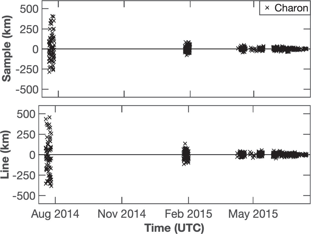
Figure 2. The Sample and Line residuals for Charon astrometry obtained by New Horizons optical navigation. The residuals were scaled by the spacecraft's distance from the Pluto system in order to express the statistics in kilometers. The rms of the residuals for three clusters of data, 2014 July, 2015 January–February, and 2015 April–July are: 167, 38, and 14 km for Sample and 217, 51, and 16 km for Line. Alternatively, the residuals in angular units are: 81, 39, and 126 mas for Sample and 105, 53, and 158 mas for Line. The same residuals in pixels are: 0.079, 0.038, and 0.123 for Sample and 0.103, 0.052, and 0.154 for Line. The resolved images of Charon occur after 2015 April and the last cluster of data has rapidly changing conversion factor for kilometers per pixel.
Download figure:
Standard image High-resolution imageWe also investigated how the correction to Pluto's planetary ephemeris influenced the residuals. We applied a linear correction to JPL's DE440 using the solution covariance as a priori (R. Park 2024, private communication). This reduced the rms for Gaia residuals to 1.05 mas with a mean of −0.26 mas (Figures 3(E) and (F)). This fit did not involve any albedo or other center-of-light, center-of-figure offsets. The planetary ephemeris correction appeared to compensate for all biases, at least to ∼1 mas level. This result is troubling, because it shows that without high-fidelity albedo model the correction to planetary orbit could be incorrect. DE440 was central to our analysis, because this orbit solution for the Pluto's system barycenter was used for the New Horizons navigation, and any changes to this solution would require a full set of Pluto's astrometry in addition to the correction implied by the Gaia astrometry of Charon. Any overhaul of planetary ephemerides is beyond the scope of this work and it also needs further verification of Gaia data on Pluto and Charon in Gaia DR5. After all, Gaia astrometry of Charon is a small portion of a long data arc and an extensive set of observations that we use in our fit. Our Gaia data set is currently dominated by the 2019 astrometry that was not part of the Gaia DR3 release and it is possible that some of these transits will get rereduced. We can clearly state that Gaia-reported submas level uncertainties in AL direction are overly optimistic. As a result of this investigation, we used only albedo-corrected Gaia astrometry (Figures 3(C) and (D)) in our final orbit fit, achieving 1.4 mas residuals.
Tables 2 through 5 contain postfit residual statistics for Nix, Hydra, Kerberos, and Styx. We subdivided Porter & Canup (2023) astrometry into years, so that we can check for any year-to-year changes in the rms. The HST data were processed to an exceptionally high quality, and we were getting ∼1 mas fit correspondence for all but Styx. This is not surprising considering that Styx is the most challenging to measure among the four satellites.
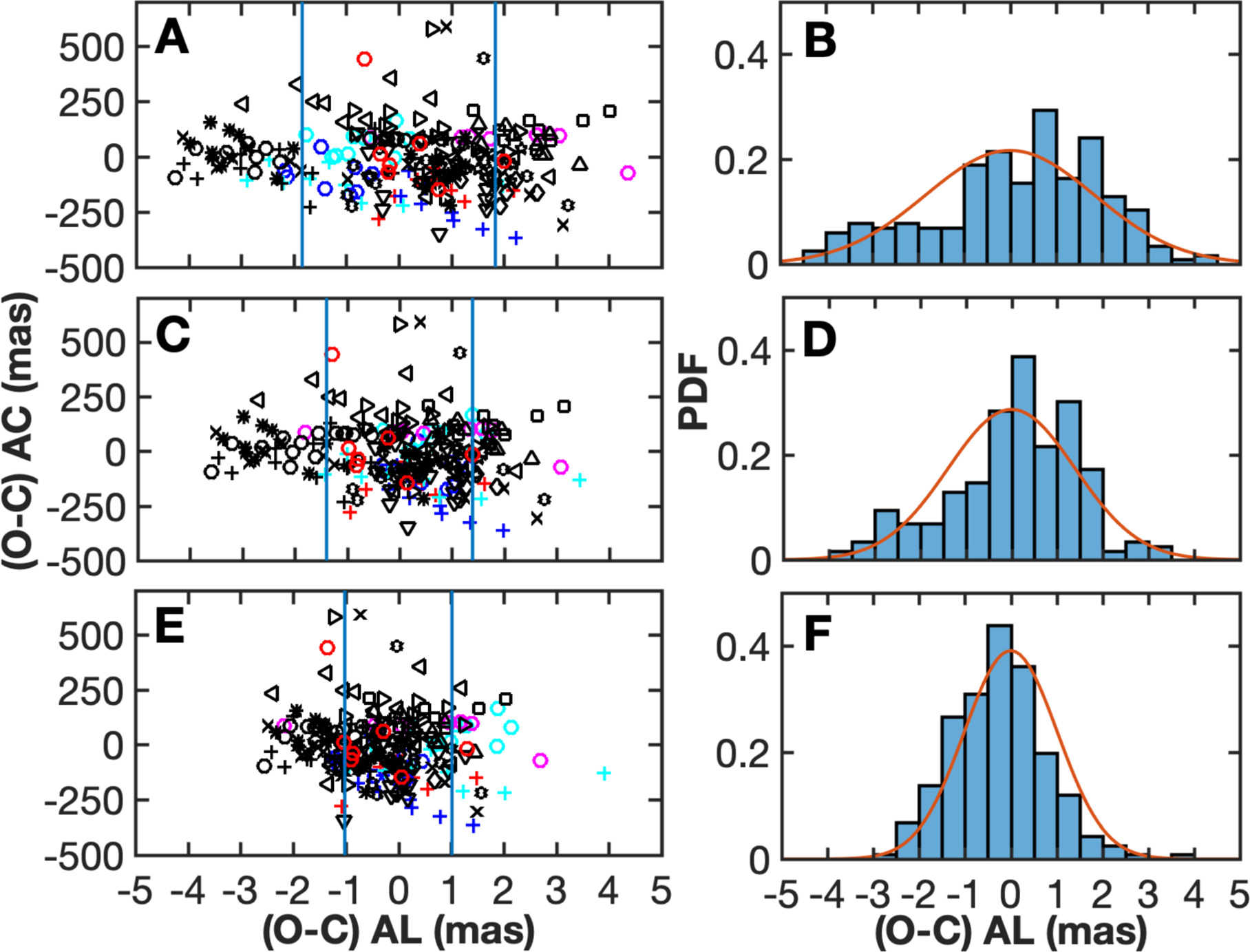
Figure 3. Residuals in AL and AC for Gaia Charon data. Different symbols and colors mark 27 Gaia transits of the object. Red, blue, cyan, magenta, and black color represent transits from 2014, 2015, 2017, 2018, and 2019. Vertical blue lines mark the 1σ of the AL residuals. (A) and (B) show residuals without albedo or planetary ephemeris biases applied. Distribution of AL residuals (232 measurements) is compared to a probability density function (PDF) for a normal distribution with zero mean (in red). (C) and (D) show the residuals for the fit with the albedo model from Buratti et al. (2017). (E) and (F) show the residuals for the fit with the corrected planetary ephemeris.
Download figure:
Standard image High-resolution imageFigure 4 shows New Horizons residuals converted to kilometers for the small satellites. Porter & Canup (2023) noted that physical resolution of the LORRI 4 × 4 (256 × 256 pixels) images is 408 pix−1 that corresponds to few thousands kilometers per pixel resolution in 2015 February and a few hundred kilometers per pixel resolution in early July. This means that the small satellites all fit within a single pixel. The weighted rms of the residuals (reduced χ2) for all New Horizons astrometry are ∼0.6, suggesting that the data were weighted slightly conservatively. We were reluctant to tighten the data weights beyond what is reported in Porter & Canup (2023), because at this level, the residuals are dominated by systematics, such as camera pointing, location of Pluto's barycenter relative to spacecraft, reduction procedure, etc.

Figure 4. Residuals for Nix, Hydra, Kerberos, and Styx astrometry obtained by New Horizons and reduced by Porter & Canup (2023). The X, Y coordinates are relative separations of the satellite and Pluto's system barycenter on the tangent plane in R.A. and decl. direction. It is equivalent to  and Δδ. The residuals were scaled by the spacecraft distance from the Pluto system in order to have kilometers as a unit. The rms of the residuals are (19, 42) km, (21, 25) km, (34, 42) km, (31, 32) km for Nix, Hydra, Kerberos, and Styx respectively. In angular unites these correspond to (131, 130) mas, (106, 114) mas, (170, 193) mas, and (206, 235) mas. For LORRI 4 × 4 images, the pixel size corresponds to 408 pix−1.
Download figure:
Standard image High-resolution image3.2. Masses
The system mass and masses of satellites were estimated together with other dynamical parameters. We obtained the following 1σ errors from the covariance of the solution: GMsys = 975.41 ± 0.09 km3 s−2 and GMCharon = 106.10 ± 0.14 km3 s−2 (Table 8). The masses agree within their statistical errors with Brozović et al. (2015). We note that Brozović et al. (2015) inflated the formal 1σ for the system and mass of Charon from GMsys = 975.2 ± 0.2 km3 s−2, GMCharon = 105.90 ± 0.3 km3 s−2 to GMsys = 975.2 ± 1.5 km3 s−2, GMCharon = 105.9 ± 1.0 km3 s−2 in order to account for potential systematic errors in the data. Our new mass estimates, obtained with a significantly more astrometry, remained consistent with Brozović et al. (2015) even within their formal bounds. We tested our results with different data weighing schemes and found that the all mass changes remained well within 3σ. It is still possible that there are some unmodeled sources of error in the data, for which we scaled the solution uncertainties by a factor of two: GMsys = 975.4 ± 0.2 km3 s−2 and GMCharon = 106.1 ± 0.3 km3 s−2. From here, the uncertainty on the mass of Pluto is GMPluto = 869.3 ± 0.4 km3 s−2 and the ratio of Charon's and Pluto's masses is mc /mp = 0.1220 ± 0.0003. We note that Null & Owen (1996) mass ratio of 0.124 ± 0.008 and Olkin et al. (2003) mass ratio of 0.122 ± 0.008 were already very close to the current estimate.
The masses of the small satellites were unconstrained by the data at the time Brozović et al. (2015) was published (JPL ephemeris PLU043). However, this did not affect the quality of the orbit fits, as the New Horizons Optical Navigation Team confirmed (Pelletier et al. 2016). We ran a comparison between PLU043 ephemeris and the orbital solution presented here (PLU060) for the time of the New Horizons flyby on 2015 July 14. The orbit difference for Charon was 2 km in radial and along the track directions and 5 km in out of plane direction. For Styx, Nix, Kerberos, and Hydra the maximum difference was always along the track: 244 km, 47 km, 106 km, and 81 km, respectively.
The new astrometry published in Porter & Canup (2023) allowed for mass determinations of Nix and Hydra, GMNix = 0.0017 ± 0.0003 km3 s−2 and GMHydra = 0.0020 ± 0.0002 km3 s−2. Our fit yields very similar values and error bars: GMNix = 0.0014 ± 0.0005 km3 s−2 and GMHydra = 0.0020 ± 0.0003 km3 s−2. We use a much larger set of parameters in the fit (over 200 including various biases) than Porter & Canup (2023) who fit only 28 parameters. Inclusion of more parameters inflates the covariance of the solution, so it is expected that our formal statistics differs. We also used a completely different orbit-fitting procedure, so it is encouraging to see that two very different methods give consistent results.
Our fit found no sensitivity for the masses of Kerberos and Styx. Section 3.2 shows that the formal fit 1σ uncertainties are  and
and  . These are factors of ∼4 and ∼13 larger than what Porter & Canup (2023) reported for their upper bounds. In order to keep our model physically realistic, we imposed 1 g cm−3 density requirement on the satellites, which yielded GMKerberos = 6 × 10⁻⁵ km3 s−2 assuming 6 km radius, and GMStyx = 4 × 10⁻⁵ km3 s−2 assuming 5.25 km radius (Porter et al. 2021). We compared the nominal orbit solution with the one where both satellites were kept massless, and we noted that the most significant effect was ∼3 km downtrack change in the orbit of Hydra. This was for the time span for which we have astrometry, 2005–2020. In other words, Kerberos and Styx are so small, that they introduce negligible perturbations on the rest of the system, at least over the period of time for which we have the data.
Table 8. Satellite Masses
| Object | Brozović et al. (2015) | Porter & Canup (2023) | Current Work |
|---|---|---|---|
| GM (km3 s−2) | GM (km3 s−2) | GM (km3 s−2) | |
| System | 975.5 ± 1.5 {0.2} | ⋯ | 975.4 ± 0.2 {0.09} |
| Pluto | 869.6 ± 1.8 | ⋯ | 869.3 ± 0.4 |
| Charon | 105.9 ± 1.0 {0.3} | ⋯ | 106.1 ± 0.3 {0.12} |
| Nix | (3.0 ± 2.7) × 10−3 | (1.75 ± 0.35) × 10−3 | (1.50 ± 0.52) × 10−3 |
| Hydra | (3.2 ± 2.8) × 10−3 | (2.01 ± 0.20)×10−3 | (2.01 ± 0.27) × 10−3 |
| Kerberos | (1.1 ± 0.6) × 10−3 | <0.05 × 10⁻³ | <0.17 × 10⁻³ |
| Styx | <1.0 × 10⁻³ | <0.03 × 10⁻³ | <0.33 × 10⁻³ |
Note. Comparison between the past and current mass estimates. The error values in the curly brackets for the system mass and the mass of Charon are the formal 1σ uncertainties from the solution covariance. These values were inflated by a factor of ∼2 to provide more conservative bounds. The fit showed no sensitivity to masses of Styx and Kerberos that were held fixed at 0.04 × 10⁻³ km3 s−2 and 0.06 × 10⁻³ km3 s−2 respectively (equivalent to density of 1 g cm−3).
Download table as: ASCIITypeset image
Table 9 compares current densities with the last two orbit fits for the Pluto system. The values for Pluto and Charon in Brozović et al. (2015) are consistent with the current work. Similarly, densities for Nix and Hydra are consistent with Porter & Canup (2023). The density limits for Nix and Hydra were not well constrained in Brozović et al. (2015) because of the order-of-magnitude masses and sizes estimates. We can tentatively put an upper bound of 2.8 g cm−3 (1σ) on the density of Kerberos, but the mass/density of Styx is cannot be constrained with the current data.
Table 9. Satellite Densities
| Object | Brozović et al. (2015) | Porter & Canup (2023) | Current Work |
|---|---|---|---|
| ρ (g cm−3) | ρ (g cm−3) | ρ (g cm−3) | |
| Pluto | 1.89 ± 0.6 [1.854 ± 0.005] | ⋯ | 1.853 ± 0.004 |
| Charon | 1.72 ± 0.02 [1.702 ± 0.017] | ⋯ | 1.705 ± 0.006 |
| Nix | <1.68 [<3.36] | 1.03 ± 0.20 | 0.88 ± 0.31 |
| Hydra | <0.88 [<3.62] | 1.22 ± 0.15 | 1.21 ± 0.19 |
| Kerberos | ⋯ | <2.03 | <2.8 |
| Styx | ⋯ | <2.20 | ⋯ |
Note. Comparison between past and current density estimates. Brozović et al. (2015) densities were calculated based on different diameters. We list in brackets the densities calculated with sizes from Stern et al. (2018) for Pluto and Charon (radii of 1188.3 ± 0.8 km and 606.0 ± 0.5 km) and from Porter et al. (2021) for Nix and Hydra (diameters of 36.5 ± 0.5 km and 36.2 ± 1.0 km). The upper bound on the density of Kerberos was calculated by adopting GM = 0.00017 (km3 s−2) from Table 8 and D = 12 km.
Download table as: ASCIITypeset image
3.3. Mean Elements
We summarize 400 yr (from 1800 January 1 to 2200 January 1) of orbit integration by calculating mean values of the elements a, e, i, and P of the osculating ellipse associated with the integrated orbit. The outline of the procedure can be found in Smart (1960), page 58. The Cartesian states were sampled once per day during this interval. Osculating period is the average sidereal period calculated from instantaneous values of  . The error bars in Table 10 reflect variations in two-body elements, as opposed to the fit uncertainties. Charon's orbit is nearly circular and its osculating period varies less than 0.2 s. The small satellites are strongly perturbed by Charon and by each other to some extent, hence their osculating elements vary in time. Styx and Nix move in the same plane as Charon, while Kerberos and Hydra have small inclinations, 0.4 deg and 0.3 deg, respectively. Figure 5 shows small variations in the osculating ellipse elements for Kerberos.
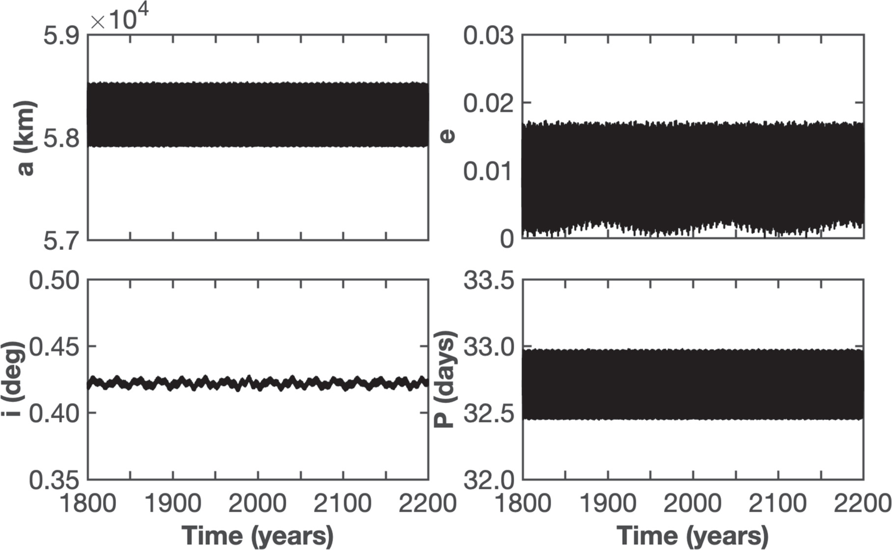
Figure 5. Osculating Keplerian elements for Kerberos from 1800 to 2200.
Download figure:
Standard image High-resolution imageTable 10. Mean Keplerian Osculating Orbital Elements for the Satellites of Pluto
| Element | Charon | Styx | Nix | Kerberos | Hydra |
|---|---|---|---|---|---|
| a(km) |

|

|

|

|

|
| e |

|

|

|

|

|
| i (deg) | ⋯ |

|

|

|

|
| P (days) |

|

|

|

|

|
Note. We list mean osculating elements where a is the semimajor axis, e is the eccentricity, i is the inclination with respect to Charon's orbit pole (see Section 3.4), and P is the orbital period. Elements for Charon are Plutocentric and elements for the small satellites are barycentric. The upper and lower bounds are based on sampling 400 yr of orbit integration (from 1800 January 1 to 2200 January 1) once per day.
Download table as: ASCIITypeset image
An alternative way to descriptively summarize integrated orbits is to apply a precessing ellipse theory as in Jacobson & Owen (2004). We sampled 400 yr of orbit integration once per day and used these positions as "measurements." The objective was to find a single set of six Keplerian elements and three rates that minimize rms of the residuals projected along the track, in radial, and out of plane directions. The optimization procedure used the least-squares method. The resulting precessing ellipse captures secular behavior of the integration, while the periodic terms are not modeled (Figure 6). The true position of Kerberos can be ∼500 km different along the track than what a simple analytical theory predicts. However, on average, the ellipse model is good. Table 11 summarizes the results. The nodal regression period for Kerberos is ∼3300 days, and it is ∼5100 days for Hydra, similar to its apsidal precession period.
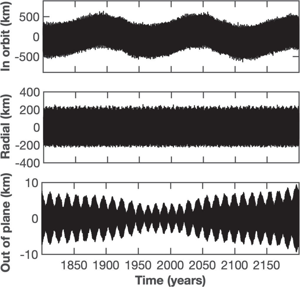
Figure 6. In orbit, radial, and out of plane differences between the integrated orbit and precessing elliptical orbit for Kerberos. Charon's orbit plane defines the reference plane.
Download figure:
Standard image High-resolution imageTable 11. Mean Precessing Ellipse Model Orbital Elements for the Satellites of Pluto
| Element | Charon | Styx | Nix | Kerberos | Hydra |
|---|---|---|---|---|---|
| a (km) | 19595.764 | 42410 | 48689 | 57749 | 64719 |
| e | 1.61 × 10⁻⁴ | ⋯ | ⋯ | ⋯ | 0.006 |
| i (deg) | ⋯ | ⋯ | ⋯ | 0.42 | 0.28 |
| n (deg day−1) | 56.362530 | 17.855 | 14.484 | 11.191 | 9.424 |
| P (days) | 6.387222 | 20.16 | 24.85 | 32.17 | 38.20 |
 (deg day−1) (deg day−1) | 2.5 × 10⁻⁶ | ⋯ | ⋯ | ⋯ | 0.070 |
 (deg day−1) (deg day−1) | ⋯ | ⋯ | ⋯ | −0.11 | −0.071 |
Note. We list mean elements according to a precessing ellipse model. This ellipse represents best fit to 400 yr of orbit integration. We only list eccentricities and inclinations if they are larger than 1 × 10⁻⁵ and 1 × 10⁻³ deg respectively. In addition to parameters in Table 10, we also estimated n, the mean longitude rate,  , the apsidal precession rate, and
  the nodal precession rate. Elements for Charon are Plutocentric and elements for the small satellites are barycentric.
Download table as: ASCIITypeset image
3.4. Charon–Pluto Orbital Plane
We were interested in examining the influence of the solar torques on the Pluto–Charon orbit plane. We used Ward (1975) and Ward & Hamilton (2004) analytical expression to estimate rate,  , at which the Charon's orbit normal is precessing about the Pluto's heliocentric orbit normal


In this expression, Q is Charon's orbit obliquity with respect to Pluto's heliocentric orbit, nCharon is orbital mean motion of Charon, n☉ is Pluto's heliocentric mean motion, sPluto is Pluto's rotation rate (same as nCharon), R is Pluto's equatorial radius, aCharon is semimajor axis of the orbit of Charon, GMPluto and GMCharon are masses of Pluto and Charon, J2 is Pluto's degree 2 zonal gravity harmonic, and γ is Pluto's normalized polar moment of inertia. For the case of Charon, the q and l terms in Equations (2) and (3) dominate over any reasonable physical values of J2 and γ in the Equation (1). We assumed J2 = 0, consistent with Pluto being a sphere, and γ = 0.4, consistent with uniform density model.
Values for semimajor axis, mean longitude rate, and Pluto's and Charon's masses can be found in Tables 11 and 8. We used 30,000 yr of JPL's DE441 planetary ephemeris (Park et al. 2021) to find mean longitude rate for Pluto's heliocentric motion (n☉ = 145.75 deg century−1) and mean obliquity of Charon's orbit (Q = 119.7 deg). For completeness, DE441 yields mean R.A. and decl. of the Pluto's heliocentric pole of 314.087 deg and 66.531 deg, apsidal regression rate of −0.00897 deg century−1, and nodal regression rate of −0.00181 deg century−1. The mean sidereal period of Pluto is 246.99 yr. We obtained a precession rate  , yielding a precession period of 9.5 million years. Consequently, Charon's orbit pole precession can be ignored in pole models spanning several thousand years.
We calculated osculating Keplerian R.A. and decl. of Charon's orbit pole for the duration of 5000 yr (Figure 7). The Sun influence is visible as a slope in R.A. and decl. There are also variations in R.A. and decl. that appear consistent with Pluto's orbital period, ∼247 yr. R.A. of the pole can be fit as R.A. = 133.0073 + 0.0036T deg, where T is Julian centuries from the epoch J2000. Decl. of the pole can be fit as decl. = –6.2449 + 2.5 × 10⁻⁵ T deg. These first-order polynomials capture the pole variations to within ∼2 millidegrees over 5000 yr.

Figure 7. Panels (A) and (B) show Keplerian osculating R.A. and decl. for Charon's orbit pole over 5000 yr starting from J2000. Panels (C) and (D) show the residuals after the removal of the linear term.
Download figure:
Standard image High-resolution image3.5. Orbital Uncertainties
Jacobson et al. (2012) showed that linear mapping of the covariance matrix obtained from a least-squares fit represents a method for placing a reasonable bound on the satellite's position at some later time. We used this method to evaluate how the positional uncertainties grow for each of the five satellites until 2050 (Figure 8). Unlike the uncertainties listed in Table 10 that represent differences between an analytical theory and true orbits, these uncertainties reflect the fit quality that is based on quantity and quality of measurements.
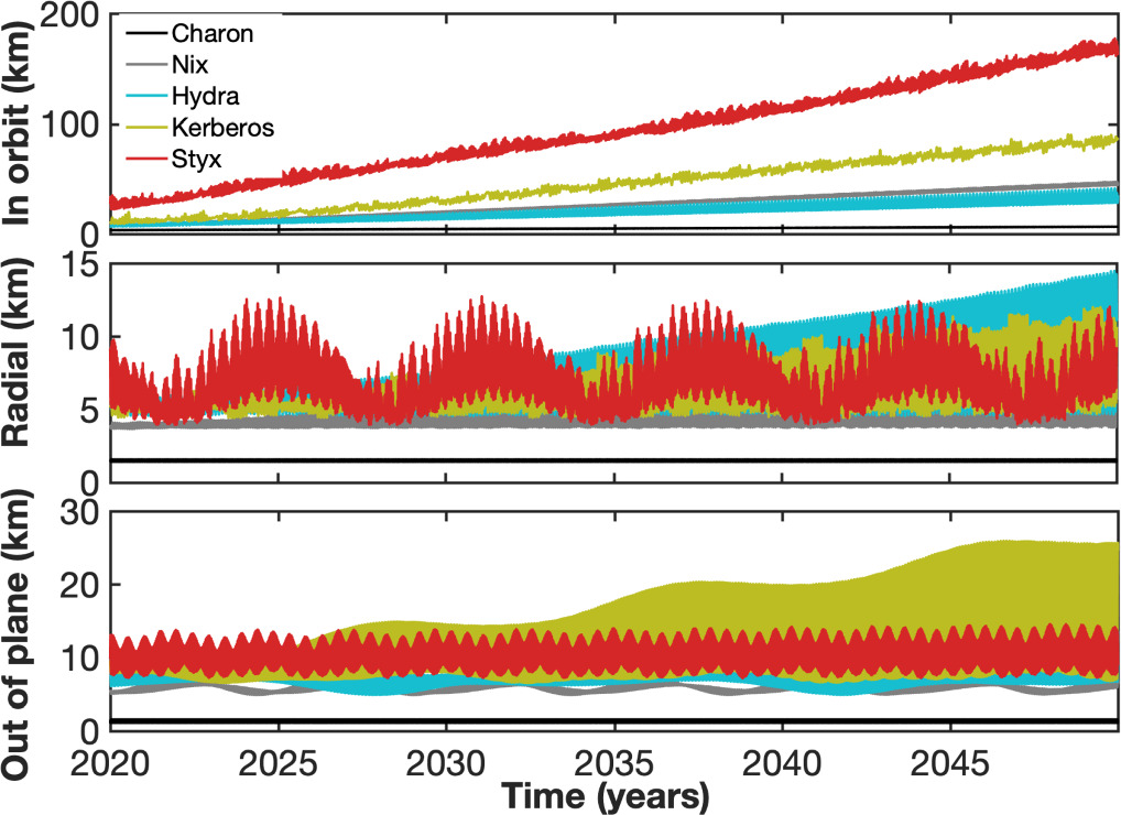
Figure 8. Orbital uncertainties for PLU060 (1σ) projected in in-orbit, radial, and out of plane directions until 2050.
Download figure:
Standard image High-resolution imageOverall, all orbits are well constrained and none of the satellites is in danger of being lost for the foreseeable future. Styx orbit has the highest uncertainty because this satellite is challenging to measure in the HST images due to its faint magnitude and proximity to the bright Pluto–Charon binary. The dominant uncertainty is always in in-orbit direction and the fit to the slopes yields the mean motion uncertainties: 9 × 10⁻⁷ deg day−1 for Charon, 2 × 10⁻⁵ deg day−1 for Styx, 4 × 10⁻⁶ deg day−1 for Nix, 7 × 10⁻⁶ deg day−1 for Kerberos, and 2 × 10⁻⁶ deg day−1 for Hydra. True uncertainties could be larger than this due to unknown systematic errors.
4. Discussion
4.1. Near Resonances
If we take the average osculating periods from Table 10, the satellites have the following ratios with respect to Charon: 3.27:3.99:5.13:6.07. If we take the periods obtained with the precessing ellipse theory (Table 11), the ratios are: 3.16:3.89:5.04:5.98. This shows that the definition of elements matters for the case of perturbed orbits, and that their interpretation (e.g., proximity to resonance) should be treated with caution.
However, taken at face value, we can note Charon–Kerberos proximity to the fourth-order inclination resonance:  . A change of 7% in the nodal precession rate would put Kerberos in a resonance. The current estimate for the nodal precession period is about nine years, and the data arc is only about 12 yr long with sparse astrometry until 2012. Thus, there is a room for improvement on the nodal precession rate. The more likely scenario is that the resonance existed in the past.
We have similar case with Charon and Hydra. Hydra has both small eccentricity and inclination, and the closest combination of the rates to a resonance that we could find is:  . The nodal and apsidal precession periods are on the order of 14 yr, and it is possible that these numbers will get revised with more data.
Showalter & Hamilton (2015) reported that Nix, Hydra, and Kerberos reside in a Laplace-like resonance. They identified 3nStyx − 5nNix + 2nHydra = − 7 ± 1 × 10⁻³ deg day−1 and suggested that the resonant argument, Φ = 3λStyx − 5λNix + 2λHydra, librates around 180 deg. Here, λ refers to mean longitude, measured from the ascending node of the Pluto–Charon orbital plane on the ICRF equator. Showalter & Hamilton (2015) noted that the resonant argument Φ decreased from 191 deg to 184 deg during 2010–2012, and that this was too coincidental to be observed by chance. However, their long-term integration showed that the libration depends on the masses of Nix and Hydra that were not well constrained at that time (Brozović et al. 2015). Showalter & Hamilton (2015) showed in their Figure 2 that the resonant argument was circulating for the case of moderate masses of Nix and Hydra (GMHydra = 0.0032 km3 s−2 and GMNix = 0.0044 km3 s−2) and that the libration condition needed several tens of percent higher mass of Hydra (Nix was already increased by 50% from Brozović et al. 2015).
We revisited this result in the light of the current orbits and masses. We obtained 3nStyx − 5nNix + 2nHydra = − 7.3 × 10⁻³ deg day−1 based on the rates from Table 11. We also calculated resonant argument based on 400 yr of osculating longitudes in Figure 9. The argument shows circulation with ∼140 yr period. The argument indeed goes through 180 deg around 2010–2012 time frame, but this does appear to be a coincidence. The lack of resonance is not surprising given the relatively "light" masses for Nix and Hydra.

Figure 9. Near resonance for Styx, Nix, and Hydra.
Download figure:
Standard image High-resolution image
4.2. Future Astrometry
We have seen in Section 3.2 that the Charon's mass was known to better than 1% even prior to the additional optical navigation measurements from New Horizons. The New Horizons astrometry further reduced this mass uncertainty by a factor of three. Regarding the small satellites of Pluto, we only have constraints on Nix and Hydra, and the principal source of mass-sensitive data are two decades of HST astrometry. The New Horizons astrometry contributed to reducing the GM uncertainty for Nix by ∼15%.
We simulated milliarcsec precision astrometry for all small satellites for the next 20 yr hoping to reveal the masses of Kerberos and Styx, but their masses remained elusive. The uncertainties were still several times larger than their expected values assuming ∼1 g cm−3 density. This is not surprising considering that the orbital differences between our nominal solution and the one where Kerberos and Styx were kept massless were small. By 2050, the in-orbit differences grow to 5 km for Styx, 6 km to Nix, 3 km for Kerberos, and 7 km for Hydra. However, more high-precision astrometry would improve the uncertainties on masses of Nix and Hydra by a factor of two, and it would also further improve their state vector uncertainties.
5. Conclusions
The satellites of Pluto have a long legacy of ground-based and the HST observations. Since 2014, Gaia spacecraft is also becoming a source of high-precision astrometry for Charon (Tanga et al. 2023), but to fully utilize that astrometry requires center-of-light, center-of-figure corrections as well as improved Pluto system planetary ephemeris. The New Horizons spacecraft collected measurements of Charon and the small satellites' as it was heading for the close flyby on 2015 July 14. Orbits and masses became better and better constrained as more and more astrometry became available (Buie et al. 2006; Tholen et al. 2008; Beauvalet et al. 2013; Brozović et al. 2015; Porter & Canup 2023). Our analysis represents the latest orbit-fitting effort where we used the most complete data set to date and a dynamical model that included all satellites as well as the external perturbers. We showed that the influence of the Sun is small, but that we still need to take it into account over longer time intervals because it is torquing the Pluto–Charon orbit plane. We determined a linear expression for the R.A. and decl. of the pole based on 5000 yr of orbit integration. The masses of Pluto and Charon are extremely well known at this point, and the latest data from Porter & Canup (2023) even helped reveal the masses of Nix and Hydra. The latest combination of orbits and masses appears to eliminate Styx–Nix–Hydra resonance that was discussed in Showalter & Hamilton (2015). Our orbit solution (PLU060) can be obtained from the JPL Horizons On-Line Solar System Data Service (Giorgini et al. 1996) and from NASA's Navigation and Ancillary Information Facility (Acton 1996).
Acknowledgments
We thank the members of the New Horizons Optical Navigation Team who allowed us to use the spacecraft astrometry for Charon. We also thank Bruno Sicardy and collaborators for giving us access to their Charon astrometry obtained by the adaptive optics system NACO/VLT at Paranal as well as two occultation points from 2011. We are very grateful to Davide Farnocchia for help with processing of Gaia astrometry and to Valery Lainey for instructive and helpful comments during the review of this paper. The research described here was carried out at the Jet Propulsion Laboratory, California Institute of Technology, under contract with the National Aeronautics and Space Administration (80NM0018D0004; Horizons 1996).
Footnotes
- 1
- 2
- 3