


Abstract
bet LMi is a double-lined visual binary with an orbital period of ∼39 yr. Via a simultaneous fitting to both astrometric and radial velocity measurements, we give a complete and improved orbit solution with high precision. Then, the component masses are precisely determined as 2.98 ± 0.10 M⊙ and 1.92 ± 0.04 M⊙ with a relative precision of ∼3%, respectively. The orbital parallax is determined to be 19.6 ± 0.2 mas, which is two times more precise than Hipparcos parallax. With the known apparent magnitudes and magnitude difference of the components, we derive the luminosity of the components as 50.7 ± 1.8 L⊙ and 9.1 ± 4.1 L⊙. The estimated radii of the components are 9.4 ± 0.3 R⊙ and 3.7 ± 1.5 R⊙.
Export citation and abstract BibTeX RIS
1. Introduction
The component masses and parallax of a binary could be determined if the binary is identified both as a double-lined spectroscopic binary and as a visual binary. The component masses would provide stringent observational tests for stellar structure and evolution models, and the orbital parallax can be used to check the parallax provided by Hipparcos and the Gaia mission as well as other methods.
The nearby star bet LMi (HD 90537, HR 4100, HIP 51233, G9III, mV = 4.21) has been known to be a binary system with a long period and large eccentricity, the components of the system were first resolved as early as in 1923 (Maggini 1925). A preliminary apparent orbit solution was given by Baize (1950), and then the orbital period (P) and the time of passage at periastron (T) were amended by Starikova (1977). As relative astrometric measurements cover more than an orbital period, Mason & Hartkopf (2001) gave the improved apparent orbit solution. Underhill (1963) identified the system as a single-lined spectroscopic binary and gave the preliminary spectroscopic elements. By combining the Hipparcos astrometry with existing ground-based observations, Söderhjelm (1999) improved the orbit solution. Gontcharov & Kiyaeva (2020) determined the photocentric orbits from a direct combination of ground-based astrometry with Hipparcos. Grifffin (2008) successfully measured the radial velocities of the secondary near the periastron and identified the system to be a double-lined spectroscopic binary. With radial velocity measurements spanning ∼40 yr, Grifffin (2008) provided a precise spectroscopic orbit solution.
At present, both the radial velocity and relative astrometric measurements have a good coverage of phase period for the system, thus an improved orbit solution can be determined. In this article, a complete orbit solution of the system is determined by a simultaneous fitting to both relative astrometric and radial velocity measurements. Meanwhile, we give the component masses and orbital parallax for the system. Then, the physical properties and the evolutionary stage of this system are determined.
2. Observation Data
2.1. Relative Astrometric Measurements
We extract the relative astrometric measurements of the two components from the Fourth Catalog of Interferometric Measurements of Binary Stars (Hartkopf et al. 2001). These data are provided by several high angle resolution methods including a visual interferometer (Wilson 1941a, 1941b, 1950, 1951; Sinton 1954), speckle interferometric technique (Morgan et al. 1978, 1980; Balega & Balega 1985, 1987; Bonneau et al. 1986; Balega et al. 1994; Miura et al. 1995; Horch et al. 2002, 2004; Scardia et al. 2005; Docobo et al. 2007; Orlov et al. 2007; Prieur et al. 2008, 2009, 2010, 2012, 2014; Losse 2010), Center for High Angular Resolution Astronomy (CHARA) speckle (McAlister 1977, 1978; McAlister & DeGioia 1979; McAlister & Hendry 1882a, 1882b; McAlister et al. 1983, 1984, 1987, 1989, 1990, 1993; McAlister & Hartkopf 1984; Hartkopf et al. 1992, 1994, 1997, 2000; Fu et al. 1997), phase grating interferometer (Tokovinin 1982a, 1982b), United States Naval Observatory (USNO) speckle (Mason et al. 2011), adaptive optics (Roberts et al. 2005), and Hipparcos observations (ESA 1997). The relative astrometric measurements mentioned above span a timeframe of ∼90 yr and has a good coverage of phase.
2.2. Radial Velocity Measurements
Based on radial velocities from 80 spectrograms, the system is identified as a single-lined spectroscopic binary and the preliminary spectroscopic orbit solution was given by Underhill (1963). Since 1970 January, Grifffin (2008) conducted spectroscopic observations of the system with equipment such as the Palomar 200 inch telescope, the Dominion Astrophysical Observatory (DAO) 48 inch telescope, and Haute-Provence Coravel (OPH), and obtained at least one radial velocity every year in the following 39 yr. Besides, he has successfully measured the radial velocities of the secondary near the periastron.
3. Orbit Determination
As two complementary types of observations, the relative astrometric measurements and radial velocity measurements can be used to determinate the complete orbit solution of a binary. The relative astrometric measurements expressed as the separation of the two components (ρ) and the position angle (θ) can be transferred to the rectangular coordinates

and the errors in the corresponding coordinates can be computed as
With a simultaneous adjustment of the fit to determine the orbit solutions of bet LMi, the objective function can be written as
N1, N2, and N3 represent the number of relative astrometric measurements, and the radial velocity of the primary and the secondary, respectively. The subscript o represents the observation, and the subscripts p and s indicate the primary and the secondary, respectively. The calculated x, y, Vp, and Vs are a function of orbit parameters, and readers can refer to Pourbaix (1998) for detailed information.
The radial velocity of bet LMi was measured by different equipment (Underhill 1963; Grifffin 2008), and the zero-point of the radial velocity measured by different equipment, and thus are probably inconsistent. Therefore, this zero-point offset is also adjusted when minimizing χ2 in Equation (1).
As Equation (1) shows, each measurement is weighted by the inverse square of its own error. For the measurements without given errors, we estimate the errors with the method proposed by Wang et al. (2015). The derived errors of radial velocities from different sources are listed in Table 1. The errors of relative astrometric measurements from CHARA speckle are given according to Table 3 of Hartkopf et al. (2000), and the minimum errors of separation are 3 mas. The mathematical expectation of the absolute value of the residuals of the same equipment is adopted as the error for the position data, e.g., the data observed by 212 cm telescope at San Pedro Martir Observatory in Mexico, and the 6 m telescope of the Special Astrophysical Observatory,] and provided by Muterspaugh et al. (2010). The errors of the other relative astrometric data are estimated from the original articles.
Table 1. Derived Errors of Radial Velocities for bet LMi from Different Sources
| Data Source | Error for the Primary | Error for the Secondary |
|---|---|---|
| (km s−1) | (km s−1) | |
| Underhill (1963) | 2.2 | ⋯ |
| Observed with original Cambridge Coravel | 0.5 | ⋯ |
| Observed with Haute-Provence Coravel | 0.3 | 1.6 |
| Observed with Cambridge Coravel | 0.3 | 0.9 |
| Observed with Palomar 200 inch telescope | 0.3 | ⋯ |
| Observed with DAO 48 inch telescope | 0.3 | ⋯ |
| Observed by Dr. J.-M. Carquillat | 0.3 | 1.1 |
| Observed by Dr. S. Udry | 0.3 | 1.0 |
| Observed by Dr. M. Imbert | 0.3 | 4.4 |
Download table as: ASCIITypeset image
A modified grid method described in Ren & Fu (2010) is used to find the global minimum of the objective function (Equation (1)). The data that lie outside 3σ confidence interval from our solution are discarded as outliers. In spite of the low accuracy of the historic visual measurements before the 1950s, including these data in the fitting lowers the error of orbital period from 43.3 to 40.3 days. The relative astrometric measurements, adopted errors, and residuals in the rectangular coordinates are shown in Table 2. The goodness of fit could be quantitatively measured by Q, which represents the probability that the χ2 should exceed a particular value by chance (Press et al. 1992). Q = 0.000428 of the fit to all the data means an acceptable solution. The Q of the fitting to the two sets of radial velocities provided by Underhill (1963), Grifffin (2008), and the relative astrometric measurements are 0.000390, 0.000118, and 0.040931, respectively. The derived orbit parameters including the radial velocity of the barycenter (V0), the amplitudes of the radial velocity curves (K1, K2), the semimajor axis of the relative orbit (a''), the inclination (i), the latitude of the ascending node (Ω), the argument of the periastron (ωA), the eccentricity (e), the period (P), and the time of passage at periastron (T) are shown in Table 3 together with orbital parallax (π'') and the component masses (M1, M2) which can be determined from the derived orbit parameters directly. Moreover, the orbit solution given by Grifffin (2008), Mason & Hartkopf (2001), Söderhjelm (1999), and Gontcharov & Kiyaeva (2020) are also shown in Table 3 for comparison. The relative astrometric measurements and the fitted apparent orbit are shown in Figure 1. The mismatch of the data from Muterspaugh et al. (2010) and the orbit implies that either the precision in Muterspaugh et al. (2010) is grossly overestimated, or there is a physical reason for these deviations. The radial velocity measurements and the fitted radial velocity curve are shown in Figure 2.
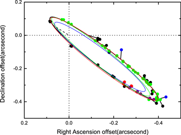
Figure 1. Apparent orbits and the relative astrometric measurements of bet LMi. The dashed line indicates the periastron. The blue dots indicate the data observed before the 1950s, and the dots in green, red, and purple indicate the observational data from CHARA speckle, provided by Muterspaugh et al. (2010), observed with the Pupil Interferometry Speckle camera and Coronagraph (PISCO) in Merate, respectively. the remaining data are shown using black dots. The black, red, green, and blue curves represent the solution given by us, Mason & Hartkopf (2001), Gontcharov & Kiyaeva (2020), and Söderhjelm (1999), respectively. Obviously, the orbit solution given by Gontcharov & Kiyaeva (2020) and Söderhjelm (1999) deviated from the observational data. Our orbit solution is similar to the one given by Mason & Hartkopf (2001) in some degree.
Download figure:
Standard image High-resolution image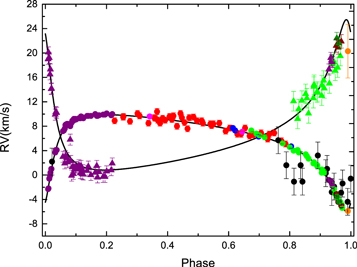
Figure 2. Fitted radial velocity curve and the observed radial velocity measurements. The dots and triangles represent the radial velocity for the primary and secondary, respectively. The black, red, green, purple, blue, magenta, wine, olive, and orange dots represent the radial velocity measurements by Underhill (1963), original Cambridge Coravel, Haute-Provence Coravel, Cambridge Coravel, DAO 48 inch telescope, Palomar 200 inch telescope, Carquillat, Udry, and Imbert, respectively.
Download figure:
Standard image High-resolution imageTable 2. Relative Astrometric Measurements, Adopted Errors, and Residuals in the Rectangular Coordinates
| Epoch of Observation | x | σx | (O − C) | y | σy | (O − C) |
|---|---|---|---|---|---|---|
| Besselian Year | (arcsec) | (arcsec) | (arcsec) | (arcsec) | (arcsec) | (arcsec) |
| 1935.3850 | −0.37159 | 0.02718 | 0.01667 | −0.43354 | 0.02796 | −0.05122 |
| 1951.3200 | −0.08714 | 0.02185 | 0.05898 | −0.23432 | 0.05261 | −0.00183 |
| 1975.9530 | −0.38730 | 0.01714 | −0.00096 | −0.35739 | 0.01734 | 0.04003 |
| 1975.9596 | −0.38412 | 0.00294 | 0.00219 | −0.39225 | 0.00294 | 0.00519 |
| 1976.0389 | −0.38901 | 0.00296 | −0.00302 | −0.39725 | 0.00296 | 0.00045 |
| 1976.2957 | −0.38553 | 0.00295 | −0.00067 | −0.39645 | 0.00295 | 0.00197 |
| 1976.3667 | −0.38132 | 0.00655 | 0.00320 | −0.38939 | 0.00661 | 0.00921 |
| 1977.0874 | −0.38623 | 0.00251 | −0.00592 | −0.39856 | 0.00254 | 0.00107 |
| 1977.1775 | −0.38754 | 0.00656 | −0.00783 | −0.40839 | 0.00672 | −0.00872 |
| 1977.3333 | −0.39244 | 0.00661 | −0.01383 | −0.39244 | 0.00661 | 0.00724 |
Only a portion of this table is shown here to demonstrate its form and content. A machine-readable version of the full table is available.
Download table as: DataTypeset image
Table 3. Improved and Published Orbit Solutions of bet LMi
| Parameter | The Present Work | Grifffin (2008) | Mason & Hartkopf (2001) | Söderhjelm (1999) | Gontcharov & Kiyaeva (2020) |
|---|---|---|---|---|---|
| K1 (km s−1) | 7.93 ± 0.05 | 7.98 ± 0.06 | |||
| K2 (km s−1) | 12.32 ± 0.18 | 13.1 ± 0.4 | |||
| ωA (deg) | 215.7 ± 0.2 | 215.6 ± 0.5 | 209.8 | 204 | 221 ± 12 |
| e | 0.680 ± 0.002 | 0.685 ± 0.004 | 0.668 | 0.69 | 0.7 ± 0.3 |
| P (days) | 13965 ± 40 | 14100 | 14106 | 14245 | 14007 |
| T (JD–2400,000) | 51411.1 ± 4.8 | 51404 ± 6 | 48525 | 50814 | 50814 |
| a'' (as) | 0.3782 ± 0.0007 | 0.363 | 0.3 | 0.36 | |
| i (deg) | 81.4 ± 0.1 | 79.1 | 79 | 81 ± 11 | |
| Ω (deg) | 40.7 ± 0.1 | 41.5 | 42 | 40 ± 15 | |
| π'' (mas) | 19.6 ± 0.2 | 22 | 22 ± 1 | ||
| M1 (M⊙) | 2.98 ± 0.10 | 1.3 ± 0.4 | |||
| M2 (M⊙) | 1.92 ± 0.04 | 1.7 ± 0.4 |
Download table as: ASCIITypeset image
4. Physical Parameters
In the Catalog of Stellar Photometry, the combined apparent magnitudes of the system in the V and R bands are 4.21 and 3.52 (Ducati 2002), respectively. The corresponding magnitude differences between the components are about 1.47 ± 0.08 and 1.78 ± 0.13 (Hartkopf et al. 2001). These imply that the apparent magnitude of the primary and the secondary in the V band are 4.40 ± 0.02 and 6.19 ± 0.08, respectively, and in the R band 3.71 ± 0.02 and 5.48 ± 0.11. According to the color index given by Houdashelt et al. (2000), we derive that the temperature of the primary and the secondary are 4097 ± 927° C and 5211 ± 843° C. Considering that the primary is much brighter than the secondary, we adopted the temperature of the primary as 5026 ± 63° C by statistics of the published temperature of the system (Glebocki 1972; McWilliam 1990; Massarotti et al. 2008; Feuillet et al. 2016; Niedzielski et al. 2016). The bolometric correction (BC) of the primary and secondary are determined as −0.295 ± 0.027 and −0.224 ± 0.481 from Flower (1996). Then, we derive the luminosity of the components as 50.7 ± 1.8 L⊙ and 9.1 ± 4.1 L⊙ respectively for the primary and the secondary. The estimated radii of the components are 9.4 ± 0.3 R⊙ and 3.7 ± 1.5 R⊙ by the Stefan–Bolzmann's law.
To investigate the evolutionary status of the two components of bet LMi, we compare the (log Teff, log L/L⊙) values of the components with the evolutionary tracks given by Girardi et al. (2000). The value [Fe/H] = 0.0 was given by McWilliam (1990) and Marfil et al. (2020), hence the metallicity of Z = 0.019 the same as the Sun is adopted. Figure 3 shows tracks of mass = 1.8, 2.0, 2.5, 3.0 M⊙ and isochrones for log(age yr−1) = 8.70, 8.75 in the (log Teff, log L/L⊙) plane. From this figure we can infer that the logarithm of the isochrone age of the system(log(age yr−1)) is about 8.72. Given the low accuracy of the luminosity and effective temperature of the secondary, we derive the luminosity as 17.6 L⊙ and effective temperature as 8380° C for the secondary corresponding to spectral type A7V at the same age with the primary, which is indicated as green dot in Figure 3. Based on the luminosity and the temperature, the radii of the secondary can be calculated as 2.0 R⊙.

Figure 3. Evolutionary tracks for the component stars and isochrones of bet LMi (Girardi et al. 2000). The solid lines and dashed lines indicate the mass tracks of 3.0, 2.0, and 1.8 M⊙ and the isochrones of log(age yr−1) = 8.75, 8.80, respectively. The red dots with error bars indicate the luminosity and temperature of both components from observation. The green dot indicates the luminosity and temperature of the secondary derived from the same isochrone as the primary's.
Download figure:
Standard image High-resolution image
5. Conclusions
When adopting a simultaneous fitting to radial velocity and relative astrometric measurements, we use all the available observation data including the latest and assign reasonable weight for those data without known error. This allows us to derive the complete and improved orbit solution of bet LMi, as well as the component masses and the orbital parallax. The component masses with a relative precision of ∼3% are completely based on the orbit parameters. The orbital parallax is 19.6 ± 0.2 mas two times more precise than Hipparcos parallax (van Leeuwen 2007). Besides, the physical parameters of the components are estimated using the combined apparent magnitudes of the system and magnitude difference.
This research has made use of the SIMBAD database (http://cdsweb.u-strasbg.fr/), the Ninth Catalogue of Orbits of Spectroscopic Binaries (SB9, http://sb9.astro.ulb.ac.be), and the double star library (http://ad.usno.navy.mil/wds/dsl.html). We thank the anonymous referee for instructive remarks. This research is supported by the National Natural Science Foundation of China under grant Nos. 11603072, 11727806, and 11673071.