


Abstract
K2-55b is a Neptune-sized planet orbiting a K7 dwarf with a radius of  , a mass of 0.688 ± 0.069
  , and an effective temperature of
  K. Having characterized the host star using near-infrared spectra obtained at IRTF/SpeX, we observed a transit of K2-55b with Spitzer/Infrared Array Camera (IRAC) and confirmed the accuracy of the original K2 ephemeris for future follow-up transit observations. Performing a joint fit to the Spitzer/IRAC and K2 photometry, we found a planet radius of
  , an orbital period of
  days, and an equilibrium temperature of roughly 900 K. We then measured the planet mass by acquiring 12 radial velocity (RV) measurements of the system using the High Resolution Echelle Spectrometer on the 10 m Keck I Telescope. Our RV data set precisely constrains the mass of K2-55b to
  , indicating that K2-55b has a bulk density of
  g cm−3 and can be modeled as a rocky planet capped by a modest H/He envelope (Menvelope = 12 ± 3% Mp). K2-55b is denser than most similarly sized planets, raising the question of whether the high planetary bulk density of K2-55b could be attributed to the high metallicity of K2-55. The absence of a substantial volatile envelope despite the high mass of K2-55b poses a challenge to current theories of gas giant formation. We posit that K2-55b may have escaped runaway accretion by migration, late formation, or inefficient core accretion, or that K2-55b was stripped of its envelope by a late giant impact.
Export citation and abstract BibTeX RIS
1. Introduction
The NASA K2 mission is continuing the legacy of the original Kepler mission by using the Kepler spacecraft to search for transiting planets orbiting roughly 10,000–30,000 stars in multiple fields along the ecliptic. Although restricted to the ecliptic plane by pointing requirements emplaced by the loss of a second reaction wheel in 2013 May, K2 has the freedom to observe a wider variety of stars than the original Kepler mission because the field of view changes every few months (Howell et al. 2014; Putnam & Wiemer 2014). The K2 target lists are entirely community-driven, and Guest Observer proposers have seized the opportunity to study planets and stars in diverse settings. K2 has already probed multiple star clusters and is surveying stars with a diverse array of ages, metallicities, and masses. Low-mass stars are particularly well represented among K2 targets: 41% of selected Guest Observer targets are expected to be M and K dwarfs (Huber et al. 2016).
The selection bias toward smaller stars is driven by the dual desires to probe stellar habitable zones and to detect small planets. Although the brief, roughly 80-day duration of each K2 Campaign window is too short to detect multiple transits of planets in the habitable zones of Sun-like stars, the window is just long enough to search for potentially habitable planets orbiting cool stars. Furthermore, the deeper transit depths of planets orbiting smaller stars increase the likelihood that K2 will be able to detect small planets using only short segments of data with relatively few transits.
As of 2018 March 28, the K2 mission had already enabled the detection of 480 planet candidates and 262 confirmed planets (NASA Exoplanet Archive K2 Candidates table, Akeson et al. 2013). In this paper, we concentrate on the confirmed planet K2-55b, a Neptune-sized planet orbiting a moderately bright late-K dwarf (V = 13.546, Ks = 10.471). Compared to a typical K2 confirmed planet, K2-55b is larger ( versus the median radius of 2.3
  ) and has a much shorter orbital period (
 days compared to the median value of 7.9 days). The host star K2-55 (EPIC 205924614) is much cooler (
 K versus 5476 K) and slightly smaller (
 versus 0.87
  ) than the average host star of a K2 confirmed planet. At [Fe/H] =0.376 ± 0.095, K2-55 is also one of the more metal-rich stars targeted by K2.
The high metallicity of K2-55 presents a convenient opportunity to test how stellar metallicity, which we assume to be a proxy for the initial metal content in the protoplanetary disk, influences the formation and evolution of planetary systems. Accordingly, the primary objective of this paper is to determine the bulk density of K2-55b and investigate possible compositional models.
Adventageously, measuring the mass of Neptune-sized planets like K2-55b also provides a way to probe the critical core mass required to commence runaway accretion and form giant planets. For larger planets, degeneracies in interior structure models typically thwart attempts to approximate core masses unless they can be inferred indirectly (e.g., via eccentricity measurements, Batygin et al. 2009; Kramm et al. 2012; Becker & Batygin 2013; Buhler et al. 2016; Hardy et al. 2017). Our secondary goal for this paper is therefore to use K2-55b as a test case for investigating the formation of massive planets.
We begin by reviewing the discovery, validation, and system characterization of K2-55b in Section 2. Next, we describe our new Spitzer and Keck/High Resolution Echelle Spectrometer (HIRES) observations of K2-55 in Section 3 and analyze them in Sections 4 and 5, respectively. We then discuss the implications of our bulk density estimate for the composition and formation of K2-55b in Section 6 before concluding in Section 7.
2. The Discovery of K2-55b
2.1. K2 Observations of K2-55
K2-55 (EPIC 205924614) was observed by the NASA K2 mission during Campaign 3, which extended from 2014 November 14 until 2015 February 3. Like the majority of K2 targets, K2-55 was observed in long-cadence mode using 30-minute integrations. The K2 photometry of K2-55 is publicly available on MAST.18
Although subsequent spectroscopic analyses have revealed that K2-55 is a dwarf star, the target was initially proposed by Dennis Stello on behalf of the KASC Working Group 8, the astroSTEP and APOKASC collaborations, and the GALAH team. Interestingly, K2-55 was not included in guest observer proposals focused on dwarf stars. For more details about the inclusion or exclusion of K2-55 in various K2 guest observer proposals, see the Appendix.
2.2. Detection and Validation of K2-55b
The K2 mission does not provide official lists of planet candidates, but K2-55b was detected by multiple teams using independent pipelines. The candidate was initially reported by Vanderburg et al. (2016) as a 4.4  planet in a 2.8 day orbit around a 4237 K star with a radius of roughly 0.65
  . Vanderburg et al. (2016) calculated the stellar properties using the
  color–temperature relation from Boyajian et al. (2013) and flagged the star as a possible giant.
Schmitt et al. (2016) also reported the discovery of K2-55b as PHOI-3 b, a transiting planet with a planetary/stellar radius ratio of  and an orbital period of 2.8 days. Schmitt et al. (2016) did not characterize the host star and therefore did not report a physical planet radius for PHOI-3 b. They did obtain Keck/NIRC2 imaging to search for nearby stellar companions and reported a lack of stellar companions between 0
 25 and 200 from the target with sensitivities of Δm = 4.00 and Δm = 6.07, respectively.
K2-55b was also detected by Barros et al. (2016), who reported transit events with a depth of 0.372% and a total duration of 2.093 hr, and by Crossfield et al. (2016). In addition to rediscovering the planet, Crossfield et al. (2016) used the VESPA framework (Morton 2012, 2015) to validate K2-55b as a bona fide planet with a radius of 3.82 ± 0.32  . The Crossfield et al. (2016) false-positive analysis incorporated K-band high-contrast imaging acquired with Keck/NIRC2 and high-resolution spectra obtained with Keck/HIRES that restricted the possibility of stellar blends. Specifically, the AO imagery ruled out the presence of stars ΔmKs = 8 fainter than K2-55 at a separation of 05 and ΔmKs = 9 fainter at a separation of 1''. Similarly, a spectroscopic search for secondary stellar lines in the Keck/HIRES spectra (Kolbl et al. 2015) placed a limit of 1% on the brightness of any secondary stars within 04. Overall, Crossfield et al. (2016) calculated a false-positive probability (FPP) of 1.7 × 10⁻⁹, well below their adopted validation threshold of FPP < 1%.
2.3. Stellar Classification
In their analysis, Crossfield et al. (2016) assumed R⋆ =0.630 ± 0.050  , M⋆ = 0.696 ± 0.047
  , and Teff =4456 ± 148 K. These initial estimates were based on the optical and near-infrared photometry available in the Ecliptic Plane Input Catalog (EPIC, Huber et al. 2016).
Martinez et al. (2017) and Dressing et al. (2017a) later revised the classification of K2-55 by acquiring near-infrared spectra at NTT/SOFI (R ≈ 1000) and IRTF/SpeX (R ≈ 2000), respectively. Dressing et al. (2017a) classified the star as a K7 dwarf with  , M⋆ = 0.688 ± 0.015
  , and
, and  K. Martinez et al. (2017) reported consistent but less precise parameters of R⋆ = 0.769 ± 0.063
  , M⋆ = 0.785 ± 0.059, and Teff = 4240 ± 259 K. These temperature constraints are consistent with the estimate of 4422 K from Gaia DR2 (Gaia Collaboration et al. 2016, 2018). For the remainder of this paper, we adopt the stellar classification from Dressing et al. (2017a) with the larger mass error of ±0.069
  reported by Dressing et al. (2017b). Note that this revised stellar radius is 13% larger than the value used in Crossfield et al. (2016), suggesting that the planet is larger than previously reported by Crossfield et al. (2016).
2.4. Improved Transit Parameters
After classifying cool dwarfs hosting K2 candidate planetary systems in Dressing et al. (2017a), we combined our revised stellar classifications with new transit fits of the K2 photometry to produce a catalog of planet properties for K2 cool dwarf systems. As explained in Dressing et al. (2017b), we estimated the planet properties by using the BATMAN Python package (Kreidberg 2015) to generate a transit model based on the formalism presented in Mandel & Agol (2002). We then estimated the errors on planet properties by running a Markov chain Monte Carlo analysis using the emcee Python package (Goodman & Weare 2010; Foreman-Mackey et al. 2013).
During the transit analysis, we varied the orbital period (P), the time of transit (TC), the planet-to-star radius ratio (Rp/R⋆), the scaled semimajor axis (a/R⋆), the inclination (i), the eccentricity (e), the longitude of periastron (ω), and two quadratic limb-darkening parameters (u1 and u2). We fit for  and
and  to increase the efficiency of sampling low-eccentricity orbits (e.g., Eastman et al. 2013) and projected the limb-darkening parameters into the q1 − q2 coordinate-space proposed by Kipping (2013). We also incorporated our knowledge of the stellar density by including a prior on the scaled semimajor axis (Seager & Mallén-Ornelas 2003; Sozzetti et al. 2007; Torres et al. 2008).
In order to reduce the likelihood of systematic biases in our planet properties, we fit the K2 photometry returned by three different data reduction pipelines. First, we analyzed the photometry returned by the K2SFF pipeline (Vanderburg & Johnson 2014; Vanderburg et al. 2016) and found a planet/star radius ratio of  . Next, we re-fit the transit parameters using photometry reduced with the K2SC pipeline (Aigrain et al. 2016) and the k2phot pipeline (Petigura et al. 2015). In both cases, we found consistent planet/star radius ratios of
  and
and  , respectively.
All of these values are in agreement with the previous estimate of Rp/R⋆ = 0.0552 ± 0.0013 (Crossfield et al. 2016), which was based on fits to the k2phot photometry. Vanderburg et al. (2016) and Schmitt et al. (2016) found larger (but also consistent) values of  and
and  , respectively.
Combining the stellar radius of  (Dressing et al. 2017a) with the planet-to-star radius ratio of
  yields a planet radius of
  (Dressing et al. 2017b). Our estimate is consistent with the radius of 4.63 ± 0.40
  estimated by Martinez et al. (2017), but significantly larger than the value of 3.82 ± 0.32
  found by Crossfield et al. (2016). We attribute the planet radius discrepancy to differences in the assumed stellar radius; the revised estimates determined by Martinez et al. (2017) and Dressing et al. (2017a, 2017b) were larger than the value assumed by Crossfield et al. (2016).
3. Observations
3.1. Spitzer/Infrared Array Camera (IRAC) Photometry
In order to refine the transit ephemeris estimated from the K2 data, we observed an additional transit of K2-55b using the Infrared Array Camera (IRAC) on the Spitzer Space Telescope (GO 11026, PI Werner). We began monitoring K2-55 at BJD = 2457430.636 (2016 February 12) and collected data points every 12 s until BJD = 2457430.891 for a total observation period of 6.1 hr. Based on our previous analysis of the K2 photometry, we expected that K2-55b would begin transiting 2 hr into the requested observation window and finish egress 1.9 hr later. Our planned observation therefore included 4.2 hr of out-of-transit flux baseline to aid our analysis of the transit event.
Prior to beginning our science observations, we obtained 30 min of "pre-observation" data to allow the telescope temperature to stabilize after slewing from the preceding target (Grillmair et al. 2012). We conducted these pre-observations in peak-up mode using the Pointing Calibration and Reference Sensor to improve the positioning of K2-55 during our science observations. For both sets of observations, we elected to conduct observations in Channel 2 (4.5 μm) rather than Channel 1 (3.6 μm) due to the lower amplitude of intra-pixel sensitivity variations visible in Channel 2 data (Ingalls et al. 2012).
3.2. Keck/HIRES Radial Velocities
Between 2016 August 12 and 2016 December 25, we obtained 12 observations of K2-55 using the HIRES (Vogt et al. 1994) on the 10 m Keck I Telescope on the summit of Maunakea. HIRES is a slit-fed spectrograph and a demonstrated single-measurement precision of approximately 1.5 m s−1 for observations with a signal-to-noise ratio (S/N) of 200 and 1 m s−1 for S/N of 500 (Fischer et al. 2016). Although the spectrometer has a wavelength range of 364–797 nm, we restricted our radial velocity (RV) analysis to the 510–620 nm region covered by the iodine reference cell, which was mounted in front of the spectrometer entrance slit for all of our RV observations. Following standard California Planet Search (CPS) procedures (Howard et al. 2010), we obtained our RV observations using the "C2" decker (087 ×14'' slit) for a spectral resolution of 55,000. We terminated the exposures after 45 minutes giving an S/N pixel−1 = 60–90 near 550 nm, depending on sky conditions.
On 2016 September 22, we also obtained a higher resolution "template" observation with the iodine cell removed to aid in the process of separating the stellar and iodine spectra. Our template observation was taken using the "B3" decker (057 × 14'' slit) to reach a higher resolution of roughly 70,000. As in previous CPS publications, we determined RVs by forward-modeling the iodine-free template spectra, a high-quality iodine transmission spectrum, and the instrumental response (Marcy & Butler 1992; Valenti et al. 1995; Butler et al. 1996; Howard et al. 2009). We present the measured RVs and uncertainties in Table 1.
Table 1. Relative Radial Velocities
| Observation Date | Radial Velocity (m s−1) | ||
|---|---|---|---|
| BJD-2450000 | UT | Value | Error |
| 7612.873042 | 2016 Aug 12 | 3.66 | 1.89 |
| 7614.003359 | 2016 Aug 13 | −19.49 | 1.88 |
| 7651.986215 | 2016 Sep 20 | 26.53 | 2.2 |
| 7668.943278 | 2016 Oct 07 | 17.93 | 2.06 |
| 7678.910917 | 2016 Oct 17 | −17.57 | 2.63 |
| 7679.739888 | 2016 Oct 18 | −14.18 | 2.06 |
| 7697.863996 | 2016 Nov 05 | 28.79 | 2.17 |
| 7713.740959 | 2016 Nov 21 | −13.72 | 1.83 |
| 7718.783696 | 2016 Nov 26 | −15.18 | 2.24 |
| 7745.740906 | 2016 Dec 23 | 15.45 | 3.26 |
| 7746.727362 | 2016 Dec 24 | 8.9 | 2.51 |
| 7747.741953 | 2016 Dec 25 | −33.2 | 2.98 |
Download table as: ASCIITypeset image
4. Analysis of the Photometry
We refined the radius estimate and ephemeris of K2-55 b by fitting the transits observed by Spitzer and K2. Having already fit the K2 data separately in Dressing et al. (2017b), we began this analysis by considering the Spitzer data alone. We then conducted a simultaneous fit of both the Spitzer photometry and the K2 photometry to further constrain the properties of the planet.
4.1. Generating Light Curves from Spitzer Data
We considered a variety of fixed and variable apertures when extracting the photometric light curves from the Spitzer observations. Our investigation was motivated by previous Spitzer analyses demonstrating that a wise choice of extraction aperture can minimize the scatter and red-noise component of the resulting residuals (Knutson et al. 2012; Lewis et al. 2013; Todorov et al. 2013; Kammer et al. 2015; Benneke et al. 2017). As in earlier studies, our full photometry extraction procedure included determining and removing the sky background, estimating the position of the star on the detector array using flux-weighted centroiding, and then summing the total flux within particular circular apertures.
In the fixed case, we tested 36 aperture radii spanning the range between 1.5 pixels and 5 pixels at 0.1 pixel spacing. When exploring time variable apertures, we began by determining the scaling of the noise pixel parameter  , where In is the intensity measured in pixel n (Mighell 2005). We then rescaled the noise pixel aperture radius as
  , where we considered scaling factors 0.6 ≤ a ≤ 1.2 and shifts −0.8 ≤ c ≤ 0.4.
We also investigated whether binning the data before fitting would improve performance. For each choice of aperture, we generated eight binned versions of K2-55 photometry using between 2 and 9 points per bin for effective integration times of 24–108 s. We analyzed these data sets along with the unbinned data.
Finally, we experimented with trimming the data. As noted by Chen et al. (2018), proper trimming of pre- and post-transit data can improve the quality of fits to Spitzer data exhibiting curved systematics. We considered 21 possible trim durations ranging between 0 hr and 1 hr at either end of the light curve and allowed the ending trim duration and the starting trim duration to assume different values.
We selected the ideal binning, aperture, and pre- and post-transit trimming by fitting the Spitzer light curve using the full range of parameter choices and inspecting each fit. After extracting and trimming each light curve, we fit the systematics and transit signal as described in Section 4.2, rebinned the residuals in progressively larger bins, checked the scaling of the noise with increasing bin size, and assessed how well each fit reproduced the expected square-root noise scaling. We performed this initial parameter exploration using an eccentric model for the orbit of K2-55b (e = 0.125, ω = 196°), but the estimated transit properties are nearly identical for eccentric and circular orbits (see Section 4.3 and Table 2).
Table 2. Transit and Systematic Parameters from the Photometric Analysis
| Model | |||||
|---|---|---|---|---|---|
| Parameter | Units | Spitzer Circular | Spitzer+K2 Circular | Spitzer+K2 Fixed e | Spitzer+K2 Variable e |
| T0a | days |
|
7.96 × 10⁻⁵ ± 0.00019 |
|
|
| P | days | 2.849274 (fixed) |
|
|
|
| Rp/R⋆,K2 | ⋯ | ⋯ |

|

|

|

|
⋯ |

|

|

|

|

|
⋯ |

|

|

|

|
| i | deg |

|

|

|

|
| σK2 | ⋯ | ⋯ |

|

|

|
| σS | ⋯ |

|

|

|

|

|
⋯ | ⋯ | ⋯ | −0.10 (fixed) |

|

|
⋯ | ⋯ | ⋯ | −0.34 (fixed) |

|
| e | ⋯ | ⋯ | ⋯ | 0.125 (fixed) |

|
| ω | rad | ⋯ | ⋯ | −2.86 (fixed) |

|
Note.
aFor ease of comparison, we display the time of transit center minus BKJD = 2150.42286667.Download table as: ASCIITypeset image
For the remainder of the paper, we investigate the light curve produced using the best combination of fit parameters: a fixed aperture radius of 2.7 pixels, a binning of 3 points per bin (36 seconds per bin), a starting trim of 0.3 hr, and no trimming at the end of the light curve. As shown in Figure 1, this light curve has the lowest red-noise component and the lowest scatter of all of the light curves we considered.
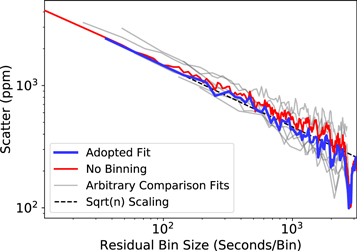
Figure 1. Performance of various fits to the Spitzer photometry compared to the expected square-root noise scaling (black dashed line). Each line displays the rms of the residuals after fitting the light curve and rebinning the residuals to bins spanning a certain number of seconds. The adopted fit (thick blue line) has both the lowest red noise and the lowest scatter. For comparison, the red line shows the performance of a fit using the same aperture and trimming but no pre-fit binning, and the gray lines show the performance of 20 other reductions of the photometry. The fits shown in light gray use different apertures, pre-fit binning, and trim durations.
Download figure:
Standard image High-resolution image4.2. Fitting the Spitzer Data
We analyzed our Spitzer data using the pixel-level decorrelation (PLD) technique first introduced by Deming et al. (2015) and later modified by Benneke et al. (2017). Specifically, we modeled the observed flux D(ti) at each timestamp ti as the multiplicative combination of a sensitivity function S(ti) and a transit model f(ti). We then maximized the likelihood
where σ is a photometric scatter parameter fit simultaneously with S(ti) and f(ti). We allowed σ to vary between 0.00001 and 0.3. For the instrument model S(ti), we assumed that the sensitivity can be described by the linear combination of the raw counts Dk (ti) of each pixel k within a 5 × 5 pixel region centered on the star and a linear ramp with slope m:
where the wk are the time-independent PLD weights given to each pixel.
We generated the transit model f(ti) by using the BATMAN python package (Kreidberg 2015) to solve the equations of Mandel & Agol (2002). Unlike the K2 photometry, our Spitzer time series contains only a single transit event. We therefore fixed the orbital period to that found by Dressing et al. (2017b) and fit for the transit midpoint T0, planet/star radius ratio Rp/R⋆, scaled semimajor axis ratio a/R⋆, and orbital inclination i. For our adopted model, we assumed that K2-55b had a circular orbit based on our analysis of the RV data (see Section 5), but we note that this choice does not significantly alter the transit profile. We estimated quadratic limb-darkening coefficients in the Spitzer bandpass by interpolating the values tabulated by Claret & Bloemen (2011). Accordingly, we set the coefficients to u1 = 0.0824 and u2 = 0.1531. We restricted the orbital inclination to 70° < i < 90° and required that the transit midpoint fall within the Spitzer data set.
In addition to verifying the orbital ephemeris predicted from the K2 data, our Spitzer data also provide an opportunity confirm the depth of the transit event. In Figure 2, we compare the planet/star radius ratios estimated from our independent fits to the K2 and Spitzer data. Although we find tighter radius ratio constraints from the K2 data ( ) than from the Spitzer data (
 ), our results are nearly identical. Table 2 contains all of the model parameters from the Spitzer-only fit.
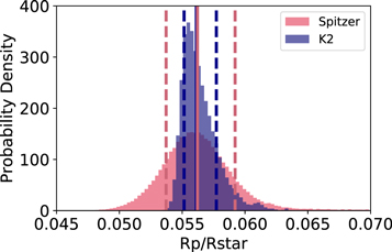
Figure 2. Comparison of planet/star radius ratios estimated by fitting the K2 (blue) and Spitzer (coral) data independently. The solid and dashed lines mark the median value and 1σ errors, respectively.
Download figure:
Standard image High-resolution image4.3. Fitting the Spitzer and K2 Data Simultaneously
After fitting the Spitzer photometry separately, we conducted a joint fit of the Spitzer and K2 photometry to further contrain the planet parameters. For our joint fit, we used fixed quadratic limb-darkening parameters set by consulting the limb-darkening tables in Claret & Bloemen (2011). Specifically, we adopted u1 = 0.7306 and u2 = 0.0338 for the Kepler bandpass and u1 = 0.0824 and u2 = 0.1531 for the Spitzer bandpass. These values are the parameters estimated by Claret & Bloemen (2011) for a 4250 K star with log g = 4.5 and [Fe/H] = 0.3.
The free parameters in our joint fit were the orbital period P, the transit midpoint T0, the planet/star radius ratio in both the Spitzer and K2 bandpasses (Rp/R⋆,Spitzer, Rp/R⋆,K2), the scaled semimajor axis ratio a/R⋆, the orbital inclination i, and two photometric scatter terms (σSpitzer, σK2). As for the Spitzer-only fit, we assumed a circular orbit for K2-55b based on our analysis of the RV data. For comparison, we repeated the analysis using an eccentric orbit (e = 0.125, ω = 196°) and found little variation in the resulting parameters. We also ran a third analysis in which we used the results of our RV analysis to impose Gaussian priors on e and ω and allowed the parameters to vary. All three fits yield consistent planet properties and Rp/R⋆,Spitzer = 0.056 ± 0.002 in all cases.
We adopt the circular fit as our chosen model and display the results in Figure 3. We also summarize the results in Table 2. The residuals to the full fit follow Gaussian distributions with a median value of −1.1 × 10⁻⁵ and a standard deviation of 0.00017 for the K2 data and 0.0001 and 0.0024, respectively, for the Spitzer data. The primary benefit to analyzing the Spitzer data along with the K2 data is that the errors on the transit midpoint and period decreased by factors of 1.9 and 4.0 compared to analyzing the K2 data alone. Accordingly, the uncertainty on the transit midpoint for an observation in late 2020 has decreased from 30 minutes to 7 minutes, significantly reducing the amount of telescope time needed to ensure that the full transit is observed.
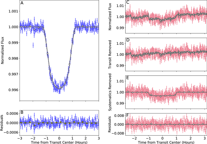
Figure 3. Joint fit to the K2 and Spitzer photometry. In all panels, the white points show the data binned to 20-minute increments. The errors on the binned data are smaller than the data points. Panel (A): Light-curve model (gray line) and phase-folded K2 photometry (blue points) vs. time. Note that the transit appears slightly v-shaped due to the relatively long 30-minute integration times used by K2. Panel (B): Residuals to the K2 fit. Panel (C): Full light-curve model (gray line) vs. raw Spitzer photometry (red points). Panel (D): Systematics model (gray) vs. Spitzer photometry after removing the best-fit transit model. Panel (E): Transit model (gray) vs. systematics-corrected Spitzer photometry. Panel (F): Residuals to the full fit.
Download figure:
Standard image High-resolution imageWe tested the influence of our choice of limb-darkening parameters by repeating the variable eccentricity analysis using two different sets of limb-darkening parameters. In particular, we considered one set of alternative parameters corresponding to a 4000 K star with log g = 4.0 and [Fe/H] = 0.2 (u1,Kepler =0.7858, u2,Kepler = −0.0163, u1,Spitzer = 0.0827, u2,Spitzer =0.1443) and a second set corresponding to a 4500 K star with log g = 5.0 and [Fe/H] = 0.5 (u1,Kepler = 0.6895,  ,
,  ,
,  ). Regardless of our specific choice of limb-darkening parameters, we found consistent results for the planet properties.
4.4. Searching for Transit Timing Variations (TTVs)
Once we had determined the best-fit system parameters, we checked for transit timing variations (TTVs) by inspecting each transit event individually. Specifically, we found the transit midpoints that minimized the difference between the observed data points and the best-fit transit model. We then rescaled the errors so that the reduced χ2 was equal to unity and slid the transit model along until the χ2 increased by 1. As shown in Figure 4, the transit midpoints we measured for the 24 transits visible in the K2 data are consistent with a linear ephemeris. Although there is a hint of curvature, fitting the transit times with a quadratic ephemeris does not improve the fit enough to justify the introduction of additional free parameters (ΔBIC = 10). Accordingly, we expected that our prediction of the Spitzer transit midpoint would be accurate to within a few hours even in the worst-case scenario. Indeed, our Spitzer-only fit yielded a transit midpoint of BJD = 2457430.75882 within one minute (<1σ) of our predicted value of BJD = 2457430.75902.
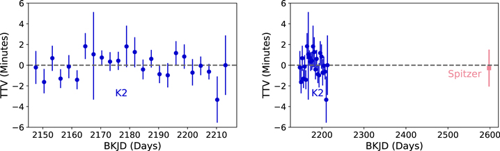
Figure 4. Observed transit times of K2-55b relative to the best-fit linear ephemeris provided in Table 4. The transit times measured from both the K2 data (blue circles in both panels) and the Spitzer data (coral square, right panel only) are consistent with a linear ephemeris. Left: Zoomed-in view of transit times measured from K2 data. Right: All measured transit times.
Download figure:
Standard image High-resolution image5. Analysis of the RV Data
As in other recent CPS publications (e.g., Christiansen et al. 2016; Sinukoff et al. 2017a, 2017b), we analyzed the RVs using the publicly available RadVel Python package19
(Fulton et al. 2018). We first performed a maximum-likelihood fit to the RVs and then determined errors by running a Markov chain Monte Carlo (MCMC) analysis around the maximum-likelihood solution. When assessing various solutions, we incorporated stellar jitter into the likelihood  by adopting the same likelihood function as Howard et al. (2014) and Dumusque et al. (2014):
where the subscript i denotes the individual data points at times ti, vi are the measured RVs, vm (ti) are the modeled RVs, σi are the instrumental errors on the measured RVs, and σsj is the stellar jitter.
RadVel conducts MCMC analyses using the affine-invariant emcee sampler (Foreman-Mackey et al. 2013) and includes built-in tests for convergence. Specifically, we initialized eight ensembles of RadVel runs each containing 100 parallel MCMC chains clustered near the maximum-likelihood solution. To ensure that the chains were well mixed and properly converged, we discarded the initial segment of each chain as "burn-in" and ran the MCMC analysis for at least 1000 additional steps. We then compared the chains across ensembles of RadVel runs and confirmed that they arrived at consistent parameter values. More formally, we tested for convergence by computing the Gelman–Rubin potential scale reduction factor  (Gelman & Rubin 1992) and requiring that
  . In order to compensate for the effects of autocorrelation on parameter estimates, we also required that our chains contained at least 1000 effective independent draws for each parameter as suggested by Ford (2006).
The K2 photometry of K2-55 revealed a single transiting planet at an orbital period of 2.85 days and no evidence for additional transiting planets. Accordingly, we began our RV fits by considering only a single planet on a Keplerian orbit. We then restricted our fits to circular orbits to test whether the additional model complexity of varying e and ω was warranted by the data. Finally, we experimented with fitting linear and quadratic trends to the data to check for the presence of additional, non-transiting planets in the system. In all cases, we fixed the stellar jitter to the value of σj = 5.34 m s−1 found when fitting the data using a single, eccentric planet.
As shown in Table 3, we found consistent masses for K2-55b regardless of whether the model included eccentricity or a long-term trend. All of these models appear to produce reasonable fits to the RV data, but they vary in the number of free parameters. In order to determine the appropriate level of complexity for our 12-point RV data set, we calculated the Bayesian information criterion (BIC, Schwarz 1978) and report the results in Table 3. Our BIC analysis revealed that the model containing a single planet on an eccentric orbit and no long-term trend fit the data better than a model containing a single planet on a circular orbit and no long-term trend, but that the additional parameters required to fit eccentric orbits were not justified by the performance of the fit (ΔBIC = 1.75). We saw no compelling evidence for a long-term variation in the data: adding a linear or quadratic trend to the eccentric planet model increased the BIC by ΔBIC = 2.48 or ΔBIC = 3.96, respectively, which indicates that the trend-free model is preferred. We display our adopted model and the Keck/HIRES data in Figure 5.
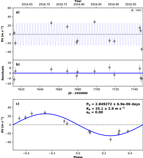
Figure 5. Top: Best-fit one-planet circular orbital model (blue line) for K2-55 overlaid on our Keck/HIRES data (circles with errors). Note that the plotted model is the maximum-likelihood model, while the orbital parameters listed in Table 4 are the median values of the posterior distributions. We add in quadrature the RV jitter term(s) listed in Table 4 with the measurement uncertainties for all RVs. Middle: Residuals to the best-fit one-planet model. Bottom: RVs phase-folded to the ephemeris of K2-55b compared to the phase-folded model.
Download figure:
Standard image High-resolution imageTable 3. RV Model Comparisona
| Model | |||||||
|---|---|---|---|---|---|---|---|
| Parameter | Units | circ | circ + linear | circ + quad | ecc | ecc + linear | ecc + quad |
| e | ⋯ | ⋯ | ⋯ | ⋯ |

|

|

|
| ω | rad | ⋯ | ⋯ | ⋯ |

|

|

|
| γ | m s−1 | 0.7 ± 2.1 | 0.7 ± 2.3 | 3.5 ± 3.2 |

|
0.6 ± 1.9 | 2.9 ± 2.9 |

|
m s−1 d−1 | ⋯ |

|
−0.027 ± 0.052 | ⋯ |

|

|

|
m s−1 d−2 | ⋯ | ⋯ | −0.0014 ± 0.0011 | ⋯ | ⋯ | −0.0012 ± 0.0011 |
| σ | m s−1 |

|

|

|

|

|

|
| K | m s−1 |

|
25.0 ± 3.2 |

|

|

|

|
| Mp |

|

|

|

|

|

|

|
| BICb | ⋯ | 87.21 | 89.69 | 89.72 | 85.46 | 87.94 | 89.42 |

|
⋯ | 1.75 | 4.23 | 4.26 | ⋯ | 2.48 | 3.96 |
Notes.
aReference epoch for γ, , and
, and  is BJD 2457689.754631.
bIn order to compute the BIC used for the model comparison, we fixed the jitter to
is BJD 2457689.754631.
bIn order to compute the BIC used for the model comparison, we fixed the jitter to  m s−1.
Download table as: ASCIITypeset image
The orbital period of K2-55b is short enough that we might have expected the orbit to be tidally circularized. According to Goldreich & Soter (1966), the circularization timescale for a planet with mass Mp and radius Rp on a modestly eccentric orbit around a star of mass  is
is

where G is the gravitational constant, a is the semimajor axis of the planet, and the factor  scales inversely with dissipation efficiency. As noted by Mardling (2007),
  is a modified Q-value and related to the tidal quality factor Q by the Love number kp such that
  .
.
We do not know the tidal quality factor or Love number of K2-55b, but adopting Neptune-like values of  (Zhang & Hamilton 2008) and
  (Burša 1992) yields circularization timescales of 110–450 Myr. These timescales are much shorter than the expected age of the system, indicating that K2-55b may actually have a higher Q if the planet really does have nonzero eccentricity. For instance, a tidal quality factor of
  would yield a circularization time of 6 Gyr.
Building on the work of Agúndez et al. (2014), Morley et al. (2017) reported a similarly high dissipation factor for GJ 436b ( ) and hypothesized that the interior structures of close-in Neptune-sized planets may differ from those of the more distant ice giants in our solar system. A high Q for K2-55b would be consistent with this theory. In the future, occasional monitoring of K2-55 over a timescale longer than our original 120 day baseline will help constrain the eccentricity and interior structure of K2-55b. For now, we adopt the circular solution and infer that K2-55b has a mass of
  . Although our model comparison test revealed that the current RV data set is better fit by an eccentric orbit than by a circular orbit, the difference is small (
 ) and the choice of a circular orbit does not significantly affect the resulting planet mass estimates (
 ).
).
6. Discussion
Now that we have constrained the radius (Section 4) and mass of K2-55b (Section 5), we devote the remainder of the paper to discussing the implications of our results. We begin in Section 6.1 by determining the bulk density of K2-55b and comparing the planet to other similarly sized planets both within and beyond the solar system. We then consider possible compositions for K2-55b in Section 6.2. When compared to other planets with similar masses or radii, we find that K2-55b has a surprisingly high density and low inferred envelope fraction.
In order to understand whether K2-55b is truly an odd planet or simply one example drawn from a class of planets with a diverse array of properties, we examine the overall frequency of intermediate-sized planets and the possible connections between planet occurrence and system properties (Section 6.3). We then review the compositional diversity of intermediate-sized planets in Section 6.4 and propose several scenarios explaining the formation of K2-55b in Section 6.5. Finally, we consider possible atmospheric models for K2-55b in Section 6.6 and discuss the prospects for follow-up atmospheric characterization studies.
6.1. Placing K2-55b in Context
Combining our photometrically derived planet radius estimate of  with our RV mass constraint of
  , we find that K2-55b has a bulk density of
  g cm−3. Although K2-55 is only 14% larger than Neptune (
 ) and 11% larger than Uranus (
 ), it is significantly more massive than either ice giant: K2-55b (
 ) is 2.5 times as massive as Neptune (
 ), three times as massive as Uranus (
 ), and nearly half the mass of Saturn (
 ). As a result, the bulk density of K2-55b (
 g cm−3) is 120% and 71% higher than the densities of Uranus (1.271 g cm−3) and Neptune (1.638 g cm−3), respectively. The interior structure of K2-55b is therefore quite distinct from that of the ice giants in our solar system. Despite the similar sizes of all three planets, K2-55b must have a lower fraction of volatiles or ices than either Uranus or Neptune.
In order to better compare K2-55b to other exoplanets, we queried the Confirmed Planets table from the NASA Exoplanet Archive20
(Akeson et al. 2013) and selected all planets orbiting single stars21
with densities measured to better than 50% as of 2018 March 28. In Figure 6, we place K2-55b and the other well-constrained planets on the mass–radius diagram. K2-55b resides near several other planets with masses  and radii
  : K2-27 b (Van Eylen et al. 2016; Petigura et al. 2017), K2-39 b (Van Eylen et al. 2016; Petigura et al. 2017), K2-98 b (Barragán et al. 2016), K2- 108 b (Petigura et al. 2017), Kepler-101 b (Bonomo et al. 2014), and WASP-156 b (Demangeon et al. 2018). All of these planets orbit stars that are hotter and more massive than K2-55. The coolest host stars are K2-39 (
 K), an evolved star with a radius of
  , and WASP-156 (
 K), a metal-rich K3 star with [Fe/H] = 0.24 ± 0.12. K2-55 stands out as the smallest, lowest mass host star harboring a massive transiting planet (
 ).
).
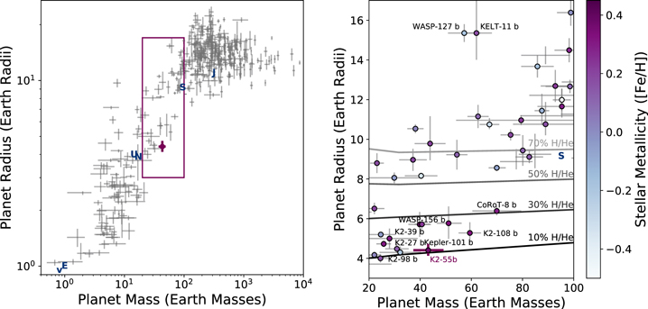
Figure 6. Mass and radius of K2-55b (point with thick purple error bars) compared to those of other small planets (points with thin gray error bars). Left: K2-55b compared to all confirmed planets from the NASA Exoplanet Archive (Akeson et al. 2013) with densities measured to better than 50% as of 2018 March 28. Right: Zoomed-in view comparing K2-55b to the subset of confirmed planets with masses between  and
and  (i.e., planets with masses within roughly a factor of two of the mass of K2-55b) and to the two-layer models from Lopez & Fortney (2014, thick gray lines). All points (including the point for K2-55b) are color-coded by the metallicity of the host star as indicated by the color bar, and the points closest to K2-55b are labeled. We also mark KELT-11b (Pepper et al. 2017) and WASP-127b (Lam et al. 2017) because they are far from the main population of planets. For reference, the purple rectangle in the left panel indicates the boundaries of the smaller region displayed in the right panel, and the navy letters in both panels mark the locations of solar system planets.
Download figure:
Standard image High-resolution image6.2. The Composition of K2-55b
The density of K2-55b ( g cm−3) is intermediate between the values expected for terrestrial planets and gas giants, suggesting that K2-55b has a heterogeneous composition containing both heavy elements and low-density volatiles. Accordingly, we model K2-55b as a two-layer planet consisting of a rocky core capped by a low-density H/He envelope. We note that that K2-55b might also contain ices (Rogers et al. 2011), but variations in the core water abundance of Neptune-sized planets have a negligible influence on the radius-composition relation compared to changes in the H/He envelope fraction. (Lopez & Fortney 2014). Furthermore, the degeneracies between icy interiors and rocky interiors are impossible to break with mass and radius measurements alone (Adams et al. 2008; Figueira et al. 2009).
For our two-layer model, we use the internal structure and thermal evolution models developed by Lopez & Fortney (2014), who generated an ensemble of model planets spanning a variety of planet masses (Mp), envelope fractions ( ), and planet insolation flux (Fp). Lopez & Fortney (2014) then evolved the planets forward in time and tracked the evolution of the planet radii. The resulting grid of planet masses, radii, envelope fractions, insolation fluxes, and ages has been used to infer the compositions of a multitude of planets (e.g., Wolfgang & Lopez 2015). The studies most germane to our analysis of K2-55b are those of Petigura et al. (2016, 2017), who employed the models of Lopez & Fortney (2014) to analyze a set of sub-Saturns. As defined by Petigura et al. (2016, 2017), "sub-Saturns" are planets with radii of
  . At
. At  , K2-55b could therefore be described as a "small sub-Saturn."
The Petigura et al. (2017) planet sample included 19 sub-Saturns with densities measured to precisions of 50% or better. Although tightly restricted in radius to  , the Petigura et al. (2017) sub-Saturn sample spans a broad mass range of
  and a correspondingly large density range of 0.09–2.40 g cm−3. The observed masses and radii of the planets in their sample could be explained by envelope fractions of 7%–60% H/He by mass.
Interpolating the same Lopez & Fortney (2014) models to investigate the composition of K2-55b, we find that our estimated mass of  and radius of
  are consistent with an envelope fraction of 12 ± 3%. This inferred envelope fraction is on the low end of the range observed by Petigura et al. (2017), underscoring the point that K2-55 has an exceptionally low gas fraction for its mass. K2-55b is denser than any of the planets in the Petigura et al. (2017) sample and more massive than all but 4 of the 19 planets they considered.
Considering all planets with  and radii of
  (i.e., all of the planets in the right panel of Figure 6), we find that the median host star has an effective temperature of 5449 K and a mass of
  . The full range spans 3416–6270 K and
  . As shown in Figure 7, the only host star less massive than K2-55 is GJ 436, further emphasizing that K2-55b may be a curiously massive planet given the mass of its host star. Figure 7 also reveals that K2-55b is denser than all of the planets in the right panel of Figure 6. The combination of our high bulk density estimate for K2-55b (
 g cm−3) and the high metallicity of K2-55 might suggest that K2-55b formed from a protoplanetary disk with an unusually deep reservoir of solid material.
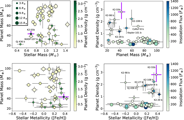
Figure 7. Comparison of the planets in the right panel of Figure 6 (circles with thin gray error bars) to K2-55b (circle with thick purple error bars). The data points are scaled by planet radius and colored by planet density (left panel) or insolation flux (right panel), as indicated by the legends. Key planets are labeled for reference. Top left: Planet mass vs. stellar mass. Top right: Planet density vs. planet mass. Note that K2-55b is the densest planet in the sample. Bottom left: Planet mass vs. stellar metallicity. Bottom right: Planet density vs. stellar metallicity.
Download figure:
Standard image High-resolution image6.3. The Frequency of Planets with Intermediate Radii
In general, Neptune-sized planets are more common than Jupiter-sized planets, but much rarer than smaller planets (e.g., Youdin 2011; Howard et al. 2012; Dressing & Charbonneau 2013; Fressin et al. 2013; Petigura et al. 2013; Fulton et al. 2017). Using the full Kepler data set and sub-dividing the stellar sample by spectral type, Mulders et al. (2015) estimated that planets with radii of  and periods of 2.0–3.4 days occur at a rate of 0.00022 ± 0.00018 planets per F star, 0.0011 ± 0.0004 planets per G star, 0.0016 ± 0.0008 planets per K dwarf, and <0.0069 planets per M dwarf. The detection of K2-55b is therefore less remarkable for the low mass of the host star than for the intermediate size of the planet: close-in Neptunes seldom occur, regardless of host star spectral type.
The dependence of the hot Neptune occurrence rate on stellar metallicity is more complicated. The increased prevalence of gas giants orbiting metal-rich stars is well established (e.g., Gonzalez 1997; Santos et al. 2004; Fischer & Valenti 2005), but the role of metallicity on the occurrence rates of smaller planets is less well understood. Examining the Kepler planet sample, Buchhave et al. (2014) found that planets larger than  orbit stars that are significantly more metal rich than the hosts of smaller planets. Buchhave et al. (2014) also noted that the host stars of 1.7–3.9
  planets are more metal rich than the host stars of smaller planets, but Schlaufman (2015) countered that the data are better described by a continuous gradient of increasing metallicity with increasing planet radius from 1
  to 4
to 4  rather than a sharp metallicity jump at 1.7
  .
.
In a related study, Wang & Fischer (2015) observed that planet occurrence is positively correlated with stellar metallicity independent of planet size. In particular, they found that metal-rich stars ([Fe/H] > 0.05) were  times more likely than metal-poor stars ([Fe/H]
  ) to harbor planets with radii of 3.9–22
  . The metallicity bias appears less pronounced for smaller planets (
 for
for  and
and  for
for  ), but the metallicity preference might be underestimated due to the observational bias against detecting transiting planets orbiting metal-rich stars due to the shallower transit depths caused by their larger radii.
Considering the possible interplay between planet occurrence, stellar metallicity, and orbital period, Mulders et al. (2016) found that short-period planets ( days) are biased toward metal-rich host stars ([Fe/H] ≃ 0.15 ± 0.05 dex) while longer period planets orbit stars with solar-like metallicities. While this trend toward higher stellar metallicities at shorter planet orbital periods is quite pronounced for the smallest planets (<1.7
  ), the trend disappears for larger planets: host stars of
  planets typically have super-solar metallicities of 0.14 ± 0.04 dex regardless of planet orbital period. Accordingly, the realization that the host star of Neptune-sized K2-55b is metal rich ([Fe/H] = 0.376 ± 0.095) would be unsurprising even if the planet had an orbital period significantly longer than the observed value of 2.8 days.
6.4. The Compositional Diversity of Planets with Intermediate Radii
Concentrating on sub-Saturns, Petigura et al. (2017) tested several different theories to explain the large dispersion in planet mass, density, and envelope fraction. Petigura et al. (2017) noted that the envelope fractions of the hottest planets in their sample ( K) were restricted to a smaller range of
  , while the cooler planets spanned the full estimated range from 10% to 60%. The lack of hot planets with larger envelope fractions might indicate that photoevaporation prevents close-in sub-Saturns from retaining large quantities of volatiles. However, photoevaporation could not be the only explanation for the observed diversity of sub-Saturn compositions because Petigura et al. (2017) did not observe a strong correlation between present-day planet equilibrium temperature and envelope fraction. In agreement with Petigura et al. (2017), the right panels of Figure 7 do not display a strong relationship between planet density and insolation flux. The most highly irradiated planet (KELT-11b, Pepper et al. 2017) has a bulk density of 0.93 g cm−3, but less strongly irradiated planets like K2-55b (
 ) span a wide range of densities from 0.09 to 2.2 g cm−3.
Similarly, Petigura et al. (2017) failed to detect a correlation between host star metallicity and envelope fraction, demonstrating that disk metallicity changes alone cannot explain the observed densities of sub-Saturns. The lack of a correlation between stellar metallicity and envelope fraction was slightly surprising because Thorngren et al. (2016) had previously noted an anticorrelation between planet metal abundance (approximated as  ) and planet mass for planets with masses of
  . The Petigura et al. (2017) planet sample included more lower mass planets than the original Thorngren et al. (2016) sample, which allowed Petigura et al. (2017) to learn that the previously detected anticorrelation does not appear to extend to planets with masses below
  . Petigura et al. (2017) suggested that perhaps the extinction of the trend at lower masses is a manifestation of different formation pathways for gas giants and lower mass planets. K2-55b is a more massive sub-Saturn and falls nicely on the relation found by Thorngren et al. (2016) between planet metal enrichment relative to stellar metallicity (
 ) and planet mass. Specifically, the Thorngren et al. (2016) relation predicts a planet metal enrichment ratio of
  for a
for a  planet, and the ratio for K2-55b is
  .
.
The high planet mass of K2-55b and the super-solar metallicity of K2-55 are also consistent with the finding by Petigura et al. (2017) that stars with higher metallicities tend to host more massive sub-Saturns. The positive correlation between stellar metallicity and sub-Saturn mass may suggest that more massive planetary cores formed in more metal-rich protoplanetary disks (Petigura et al. 2017). As shown in the bottom panels of Figure 7, the densest sub-Saturns tend to orbit the most metal-rich host stars. This trend is particularly pronounced in the bottom right panel, which displays a clear separation between the denser sub-Saturns and the low-density larger planets.
Intriguingly, Petigura et al. (2017) also noted that more massive sub-Saturns tend to have moderately eccentric orbits and orbit stars without other detected planets, while less massive sub-Saturns tend to follow more circular orbits and reside in systems with multiple transiting planets. As a  planet in a system with no other detected planets, K2-55b might therefore be expected to have an eccentric orbit. Additional observations are required to tighten the constraints on the orbital eccentricity of K2-55b and better distinguish between eccentric and circular models.
6.5. Possible Formation Scenarios for K2-55b
Under the core-accretion model of planet formation, planetesimals collide to form protoplanetary cores, which then acquire gaseous envelopes (Perri & Cameron 1974; Mizuno et al. 1978; Mizuno 1980; Stevenson 1982; Bodenheimer & Pollack 1986; Pollack et al. 1996). If the planet core is able to become sufficiently massive before the gaseous disk dissipates (at roughly a few Myr, Williams & Cieza 2011), then the growing planet can enter a phase of runaway accretion in which the envelope grows rapidly. The onset of the "core-accretion instability" occurs when the mass of the planetary core exceeds the "critical core mass," Mcrit. While numerous studies have estimated Mcrit as roughly  (Ikoma et al. 2000, and references therein), Rafikov (2006, 2011) demonstrated that variations in the assumed disk properties and planetesimal accretion rate can alter Mcrit by orders of magnitude, resulting in a wide range of
  . In general, Mcrit decreases with increasing distance from the star due to the cooler disk temperatures found in the outer disk. Mcrit also decreases with increasing mean molecular weight, but this effect can be outbalanced by the stronger trend of increasing Mcrit with increasing dust opacity (Hori & Ikoma 2011; Nettelmann et al. 2011; Piso & Youdin 2014).
Although the mass of K2-55b is below the upper end of the  range found by Rafikov (2006, 2011), the absence of a large volatile envelope for a
  planet is noteworthy and at odds with general expectations from core-accretion models. Naïvely assuming that K2-55b formed in situ at 0.0347 au in a minimum mass solar nebula (MMSN, Hayashi 1981) with a
  solid surface density profile, a total mass ratio F = 1, and a metal richness
  (Chiang & Youdin 2010), there would have been only
  of solids available for building K2-55b. Adopting a more massive minimum mass extrasolar nebula (MMEN) solid surface density profile (Chiang & Laughlin 2013; Gaidos 2017) would yield roughly
  of solids. Although significantly higher than the estimate based on the MMSN, the solid mass locally available in the MMEN model is lower than 0.4% of the present-day mass of K2-55b, indicating that either K2-55b itself or the planetary building blocks that would become K2-55b (e.g., Hansen & Murray 2012; Chatterjee & Tan 2014) must have migrated inward from farther out in the disk.
Acknowledging the puzzling existence of a massive close-in planet with only a modest H/He envelope, we propose four possible formation scenarios for K2-55b:
- 1.Classic type I migration into the inner disk cavity
- 2.Collisions of multiple planets
- 3.Post-formation atmospheric loss
- 4.Formation via less efficient core accretion.
Under the first scenario, uneven torques from the disk on K2-55b would have caused the planet to drift inward toward the host star (Ward 1997; Tanaka et al. 2002). The type I migration22 would have been halted after K2-55b entered the inner cavity between the disk and the star. K2-55b would have therefore escaped runaway accretion because it was trapped at the 2:1 resonance with the disk inner edge (e.g., Kuchner & Lecar 2002) rather than embedded within the disk. Although feasible, this argument is unsatisfying due to the fine-tuning required to have K2-55b cross the disk edge after reaching a high overall mass but before accumulating a substantial envelope.
In the second scenario, K2-55b might have been formed via collisions of smaller planets. For instance, Boley et al. (2016) found that collisions of smaller planets in systems of tightly packed inner planets (STIPs) can produce gas-poor giant planets if the progenitor planets collide after the gas disk has dissipated. Another possible explanation is that the protoplanetary disk orbiting K2-55 might have been slightly misaligned with respect to the host star (e.g., Bate et al. 2010), which could have been orbited by several less massive planets. Once the gas in the disk had dissipated, the continued contraction of the star along the Hayashi track could have driven a resonance through the system (Spalding & Batygin 2016). The resonance would have perturbed the orbits of the smaller planets, causing them to collide with each other and form a more massive planet.
The primary challenge facing the second explanation is that collisional velocities close to the star at the present-day orbital location of K2-55b are high enough that collisions are more likely to result in fragmentation than growth (Leinhardt & Stewart 2012, but see Wallace et al. 2017). Unless the smaller planets collided farther out in the disk where collisional velocities were lower and the newly formed K2-55b subsequently migrated inward to 0.0347 au via planetesimal scattering, this scenario is unlikely to explain the formation of K2-55b. Alternatively, the presence of a gaseous envelope before the collision might have made the collision less destructive (e.g., Liu et al. 2015). The logical observational test for this scenario is to measure the spin–orbit alignment of the system via the Rossiter–McLaughlin effect (McLaughlin 1924; Rossiter 1924), but the host star is too faint to permit such a precise measurement with current facilities.
A third possibility is that K2-55b formed as a "regular" sub-Saturn with a typical envelope fraction but then lost most of its envelope to a single late giant impact (e.g., Inamdar & Schlichting 2015, 2016; Liu et al. 2015; Schlichting et al. 2015). More massive planets are less vulnerable to envelope loss via either photoevaporation or impacts (Lopez & Fortney 2013; Inamdar & Schlichting 2015), suggesting that a late giant impact could have had a more catastrophic effect for K2-55b than for a Saturn-mass planet.
Our fourth formation scenario for K2-55b is that the planet formed via "conventional" core accretion, but that our incomplete understanding of core accretion causes us to overestimate the efficiency of planet formation. We note that the relatively small envelopes of Uranus and Neptune mandate that the gas disk dissipated just after the planets reached their final masses (e.g., Pollack et al. 1996; Dodson-Robinson & Bodenheimer 2010) and that producing super-Earths rather than mini-Neptunes requires delaying planet formation until most of the gas is depleted (Lee et al. 2014; Lee & Chiang 2016). Alternatively, super-Earths might form in a gas-rich disk but with dust-rich atmospheres that delay cooling and prevent them from acquiring enough gas to trigger runaway accretion (Lee et al. 2014; Lee & Chiang 2015).
Instead of requiring that the gas in the K2-55 protoplanetary disk dissipated just as K2-55b was beginning to accrete an envelope, an alternative formation scenario is that K2-55b grew via pebble accretion (Lambrechts & Johansen 2012). As the pebbles accreted, they would have heated the growing planet and consequently turned to dust due to the high temperature of the atmosphere. The dusty atmosphere would have inhibited cooling and prevented K2-55b from accreting an envelope (Lega & Lambrechts 2016).
Although the pebble heating explanation is appealing, Lee & Chiang (2015) note that pebble accretion can block runaway accretion only for planets with low-mass cores ( ); a youthful version of K2-55b would be too massive to escape runaway gas accretion. Nevertheless, the modern high density of K2-55b might be attributed to gas-stealing late giant impacts (Inamdar & Schlichting 2015, 2016). If K2-55b actually has an eccentric orbit, tidal heating may have also warmed the planet and helped block runaway accretion (Ginzburg & Sari 2017). While the specific formation pathway for K2-55b is uncertain, the sheer variety of possible explanations demonstrates that further theoretical and observational work is required to better understand core accretion and planet formation in general. Studying additional planets in the same size range as K2-55b will help determine which scenario (or combination of scenarios) best explains the formation of dense Neptune-sized planets.
6.6. Prospects for Atmospheric Investigations
Although K2-55b alone cannot solve all of the mysteries of planet formation, determining the composition of the envelope may help constrain where and how K2-55b formed. At the most basic level, determining the mean molecular weight of the atmosphere would reveal whether our simplistic two-layer model of a rocky core surrounded by a H/He envelope is sufficient or whether K2-55b is better explained by a lower-density core containing a large admixture of ices and a higher-density water-rich envelope. More sophisticated measurements of the relative abundances of particular molecules would enable tests of the various formation scenarios outlined in Section 6.5 and perhaps spur the genesis of new formation scenarios. For instance, measuring a superstellar C/O ratio would provide further evidence that K2-55b formed beyond the snow line and subsequently migrated inward (Öberg et al. 2011). On the other hand, measuring a substellar C/O ratio could indicate that K2-55b formed inside the ice line (Mordasini et al. 2016).
Transmission spectra would also reveal whether the atmosphere of K2-55b is clear or shrouded by clouds or hazes. Morley et al. (2015) predicted a transition at equilibrium temperatures near 1000 K between predominantly hazy atmospheres for cooler planets and predominantly clear atmospheres for hotter planets. Crossfield & Kreidberg (2017) note that observations of warm Neptunes ( ,
,  ) are consistent with this theory, but that the observations cannot yet differentiate between high mean molecular weight atmospheres and high-altitude clouds or hazes for the majority of planets with apparently featureless spectra. Furthermore, the Crossfield & Kreidberg (2017) sample contains only six warm Neptunes. K2-55b has an equilibrium temperature of roughly 900 K and would be an interesting addition to this small sample.
In order to test whether such observations might be feasible, we used the publicly available ExoTransmit package (Kempton et al. 2017) to generate model atmospheres for K2-55b. We considered a wide variety of atmospheric compositions with a range of C/O ratios. In all cases, the high surface gravity of K2-55b ( ) muted the dynamic range of atmospheric features, rendering detailed atmospheric characterization challenging.
Overall, the full range of transit depths is expected to span approximately 150 ppm if the atmosphere has roughly solar composition. Increasing the C/O ratio of a solar metallicity model atmosphere from C/O=0.2 to C/O=1.2 would increase the transit depth by 50–100 ppm in the most informative regions (2–2.5 μm and 3–4 μm) and produce negligible effects elsewhere in the spectrum. Distinguishing between a water-dominated atmosphere and a carbon dioxide-dominated atmosphere would require detecting differences of roughly 20 ppm. Accordingly, the first-order investigation of whether the atmosphere of K2-55b has a low or high mean molecular weight would be relatively straightforward (assuming that the investigation is not foiled by clouds), but determining detailed molecular abundances would require a more significant investment of telescope time.
The atmosphere of K2-55b could also be probed during secondary eclipse. Assuming an albedo of 0.15 and an equilibrium temperature of 900 K, the estimated secondary eclipse depth is 140 ppm. This modest signal would be challenging to detect with Spitzer (S/N = 0.8), but would be detectable with MIRI on board the James Webb Space Telescope (S/N = 7–8). For reference, GJ 436b has a secondary eclipse depth of 155 ± 22 ppm at 3.6 μm (Morley et al. 2017), but GJ 436 (V = 10.613, Ks = 6.073) is significantly brighter than K2-55 (V = 13.55, Ks = 10.471).
7. Conclusions
By adding new Spitzer/IRAC and Keck/HIRES observations to extant K2 and IRTF/SpeX data, we have investigated the composition and formation of K2-55b, a Neptune-sized planet orbiting a metal-rich K7 dwarf. Our Spitzer/IRAC data confirmed that K2-55b does not exhibit TTVs and verified the accuracy of the K2 ephemeris for future transit observations. Our Keck/HIRES data revealed a high mass of  , which resulted in a bulk density estimate of
  g cm−3 when combined with the radius estimate of
  from our joint fit to the K2 and Spitzer photometry. By comparing our mass and radius estimates to theoretical models (Lopez & Fortney 2014), we found that K2-55b can be described by a rocky core surrounded by a modest H/He envelope comprising 12 ± 3% of the total planet mass. The full system parameters are displayed in Table 4.
Table 4. K2-55 System Parameters
| Parameter | Value and 1σ Errors | References |
|---|---|---|
| K2-55 (star) = EPIC 205924614 | ||
| R.A. |

|
1 |
| Decl. |

|
1 |
| V magnitude | 13.546 | 1 |
| Kepler magnitude | 13.087 | 1 |
| 2MASS K magnitude | 10.471 | 1 |
 (K) (K) |

|
2 |

|

|
2 |

|
0.688 ± 0.069 | 2 |
![$[\mathrm{Fe}/{\rm{H}}]$](https://content.cld.iop.org/journals/1538-3881/156/2/70/revision1/ajaacf99ieqn211.gif)
|
0.376 ± 0.095 | 2 |

|
4.566 ± 0.036 | 2 |
| Systemic Velocitya(m s−1) | 0.7 ± 2.1 | 6 |
| RV Jitter (m s−1) |

|
6 |
| Parallax (mas) | 6.240 ± 0.028 | 4 |
| Distance (pc) |

|
5 |
| K2-55b (planet) = EPIC 205924614.01 | ||
| Transit and orbital parameters | ||
| Orbital period P (days) |

|
6 |
| Transit epoch TC (BJD) | 2456983.4229 ± 0.00019 | 6 |
| a (au) | 0.0347 ± 0.001 | 3 |
| Rp/R⋆ |

|
6 |
| a/R⋆ |

|
6 |
| Inc (deg) |

|
6 |
| Impact parameter |

|
6 |
| Longitude of periastron ω (rad) | fixed to 
|
6 |
| Orbital eccentricity e | fixed to 0 | 6 |
| RV semi-amplitude K (m s−1) |

|
6 |
| Planetary parameters | ||
Rp ( ) ) |

|
6 |
Mp ( ) ) |

|
6 |
 (g cm−3) (g cm−3) |

|
6 |
Fp ( ) ) |

|
3 |
 (K)b (K)b
|
900 | 6 |
| H/He envelope fraction | 12 ± 3% | 6 |
Notes.
aSystemic velocity at BJD 2457689.754631. bAssuming a Bond albedo of 0.15.References. (1) Huber et al. (2016), (2) Dressing et al. (2017a), (3) Dressing et al. (2017b), (4) Gaia Collaboration et al. (2018), (5) Bailer-Jones et al. (2018), (6) This Paper.
Download table as: ASCIITypeset image
Although the envelopes of many similar sized planets contain up to 60% of the total planet mass (Petigura et al. 2017), only 10% of the mass of K2-55b is expected to reside in the envelope. The relatively low envelope fraction was surprising because the estimated core mass of K2-55b is significantly higher than the typically quoted value of  required to spur runaway accretion (Ikoma et al. 2000). We proposed four possible explanations for the absence of a massive envelope: (1) K2-55b drifted into the inner cavity of the disk via type I migration just as the envelope was starting to accumulate; (2) K2-55b formed via the collisions of multiple smaller planets after the gas disk dissipated; (3) K2-55b formed with a substantial envelope that was later removed by a giant impact; and (4) K2-55b appears unusual only because our understanding of core accretion is incomplete.
Distinguishing among these scenarios (and others not listed here) will require expanding the sample of Neptune-sized planets with well-constrained densities. Fortunately, there are multiple pathways to find those planets. The NASA K2 mission is currently searching for transiting planets orbiting tens of thousands of stars in the ecliptic plane, including some cool dwarfs with high metallicities, and more ground-based surveys are beginning operations each year. Although many RV-detected planets will not transit and are therefore poor targets for compositional analyses, knowledge of the orbital periods and approximate masses of non-transiting planets still informs models of planet formation and evolution.
Beginning later this year, the NASA Transiting Exoplanet Survey Satellite (TESS, Ricker et al. 2014) will conduct a nearly all-sky survey for transiting planets orbiting nearby bright stars. Due to the wide-field nature of the survey, TESS will naturally survey stars with a wide range of metallicities and masses. In the late 2020s, the ESA PLATO mission (Rauer et al. 2014) will uncover even more transiting planets orbiting bright stars and precisely constrain host star properties using asteroseimology. Future follow-up observations with extremely precise RV spectrographs will constrain the masses of transiting planets and permit further investigations of the correlations of the compositions of Neptune-sized planets and the minimum mass required to instigate runaway accretion. Atmospheric investigations with the JWST, the Hubble Space Telescope (HST), and Spitzer will be particularly useful for tracing present-day planet properties backward to formation scenarios.
This work was performed in part under contract with the Jet Propulsion Laboratory (JPL) funded by NASA through the Sagan Fellowship Program executed by the NASA Exoplanet Science Institute. C.D.D., A.W.H., and I.J.M.C. acknowledge support from the K2 Guest Observer Program. A.W.H. acknowledges support for our K2 team through a NASA Astrophysics Data Analysis Program grant and observing support from NASA at Keck Observatory. E.A.P. acknowledges support from Hubble Fellowship grant. We thank the anonymous referee for providing helpful comments that improved the quality of the paper.
This paper includes data collected by the K2 mission, which is funded by the NASA Science Mission directorate. The W.M. Keck Observatory is operated as a scientific partnership among the California Institute of Technology, the University of California and the National Aeronautics and Space Administration. The Observatory was made possible by the generous financial support of the W.M. Keck Foundation. This work is based in part on observations made with the Spitzer Space Telescope, which is operated by the Jet Propulsion Laboratory, California Institute of Technology under a contract with NASA. This research has made use of the NASA Exoplanet Archive, which is operated by the California Institute of Technology, under contract with the National Aeronautics and Space Administration under the Exoplanet Exploration Program.
This work has made use of data from the European Space Agency (ESA) mission Gaia (https://www.cosmos.esa.int/gaia), processed by the Gaia Data Processing and Analysis Consortium (DPAC, https://www.cosmos.esa.int/web/gaia/dpac/consortium). Funding for the DPAC has been provided by national institutions, in particular the institutions participating in the Gaia Multilateral Agreement.
The authors wish to recognize and acknowledge the very significant cultural role and reverence that the summit of Maunakea has always had within the indigenous Hawaiian community. We are most fortunate to have the opportunity to conduct observations from this mountain.
Facilities: IRTF (SpeX) - , Keck:I (HIRES) - , Spitzer (IRAC). -
Software: emcee (Foreman-Mackey et al. 2013), ExoTransmit (Kempton et al. 2017), RadVel (Fulton et al. 2018).
Appendix: The Inclusion and Exclusion of K2-55 in K2 Guest Observer Programs
Although K2-55 is a dwarf star, it was not included in any of the approved K2 Guest Observer programs focused on dwarfs. In this section, we explore why K2-55 was proposed as part of a program focused on giant stars and excluded from programs studying dwarf stars. We first review the selection criteria for K2GO3051 (the program that nominated K2-55) and then consider three large programs focused on cool dwarfs.
K2GO3051 (PI: Dennis Stello) is a galactic archeology program designed to probe the chemical evolution of the Milky Way via asteroseismology of red giants. Stello and collaborators selected their targets using a color–magnitude cut. They first restricted the sample to all stars redder than J − Ks = 0.5 and then ranked stars in order of decreasing brightness. While 90% of the selected stars are expected to be giants, the proposers noted that their sample also includes red M and K dwarfs. The inclusion of K2-55 in the K2GO3051 target list is therefore unsurprising, but its absence in any of the large Campaign 3 proposals targeting cool dwarfs (GO3069, GO3106, GO3107) is more noteworthy.23
K2-55 met the proper motion requirement of >5 mas yr−1, the color cut of 0.7 < J − K < 1.1, and the brightness requirement of r < 17 in the Carlsberg Meridian Catalogue (Muiños & Evans 2014) required by B. Montet and collaborators for inclusion in GO3069, but the target failed the second color cut of r − J > 2.0. The r − J color of K2-55 is  .
.
K2-55 was likely excluded from GO3106 and GO3107 because of its modest proper motion: −14.9 mas yr−1 in R.A., −22.1 mas yr−1 in decl. (UCAC4, Zacharias et al. 2013). For GO3106, C. Beichman and collaborators crossmatched the 2MASS and WISE catalogs and selected targets based on both colors and reduced proper motions. Beichman et al. supplemented their target list by adding additional bright cool dwarfs from SIMBAD and SDSS. Finally, I. Crossfield, J. Schlieder, and S. Lepine proposed 4545 small stars for GO3107 by selecting targets from the SUPERBLINK proper motion survey (Lépine & Shara 2005; Lépine & Gaidos 2011) and prioritizing them by planet detectability.
Footnotes
- *
Some of the data presented herein were obtained at the W. M. Keck Observatory, which is operated as a scientific partnership among the California Institute of Technology, the University of California, and the National Aeronautics and Space Administration. The Observatory was made possible by the generous financial support of the W.M. Keck Foundation.
- 18
- 19
- 20
- 21
We omitted the circumbinary Kepler-413b from Figures 6 and 7. Although Kepler-413b may resemble K2-55b in terms of mass, radius, and bulk density (
 g cm−3), the two planets likely followed different formation pathways. Furthermore, Kepler-413b has only coarse mass constraints based on photometric-dynamical modeling (Kostov et al. 2014).
 - 22
For a recent review of type I migration and disk–planet interactions in general, see Kley & Nelson (2012).
- 23
Note that there is no requirement that K2 target lists cannot overlap. On the contrary, many selected K2 targets were proposed by multiple teams.

