


Abstract
We present a time-variability study of young stellar objects (YSOs) in the Serpens South cluster performed at 3.6 and 4.5 μm with the Spitzer Space Telescope; this study is part of the Young Stellar Object VARiability project. We have collected light curves for more than 1500 sources, including 85 cluster members, over 38 days. This includes 44 class I sources, 19 sources with flat spectral energy distributions (SEDs), 17 class II sources, and five diskless YSO candidates. We find a high variability fraction among embedded cluster members of ∼70%, whereas young stars without a detectable disk display no variability. We detect periodic variability for 32 sources with periods primarily in the range of 0.2–14 days and a subset of fast rotators thought to be field binaries. The timescale for brightness changes are shortest for stars with the most photospheric SEDs and longest for those with flat or rising SEDs. While most variable YSOs become redder when fainter, as would be expected from variable extinction, about 10% get bluer as they get fainter. One source, SSTYSV J183006.13−020108.0, exhibits "cyclical" color changes.
Export citation and abstract BibTeX RIS
1. Introduction
Circumstellar disks are an ubiquitous product of star formation, as revealed by the plethora of young stellar objects (YSOs) with mid-IR excesses detected by the Spitzer Space Telescope (Allen et al. 2004; Churchwell et al. 2009; Evans et al. 2009). These disks mediate mass accretion and angular momentum loss in pre-main-sequence (PMS) stars and also represent the immediate environment for planet formation. Understanding the physical properties and evolutionary paths of these disks is central to constructing viable models of the formation of stars and planets. Photometric variability was one of the original identifying characteristics of YSOs, even before the source stars were known to be young (Joy 1946). Optical monitoring is primarily sensitive to events and features near the stellar photosphere; such studies have determined the rotational periods of YSOs (e.g., Rydgren & Vrba 1983) and the sizes, temperatures, and temporal stability of hot and cold spots on YSO photospheres (e.g., Bouvier et al. 1986). However, the embedded nature of many YSOs favors monitoring in near- and mid-IR wavelengths, especially to study changes in the inner disk.
Studies of the Taurus, Orion, and Chameleon I molecular clouds established that near-IR variability is present in YSOs (Skrutskie et al. 1996; Carpenter et al. 2001, 2002). In the Orion Nebula Cluster, Rice et al. (2015) identified more than a thousand variable YSOs, including over 500 periodic sources in their JHKs survey. They found the observed color changes to be correlated with the observed periods, indicating both disk absorption and accretion phenomena.
Given the temperature profile of a protoplanetary disk, we can observe processes at the inner rim of the disk in the near-infrared (J, H, and K bands) since the inner edge of the disk is determined by the dust sublimation temperature of ∼1500 K, and the blackbody radiation from a part of the disk with that temperature peaks around 2 μm. However, not all circumstellar disks are manifested at the H and Ks bands. In the Orion Nebula Cluster, Lada et al. (2004) noted the fraction of disked stars more than doubles when using 3.8 μm excesses instead of relying on K-band data alone. Observations in the infrared from ∼3 to 5 μm provide observational access to parts of the disk with surface temperatures of 700–800 K.
The Young Stellar Object VARiability project (YSOVAR; Rebull et al. 2014, hereafter Paper I) has obtained extensive, multiwavelength time series photometry over 40–700 day intervals for >1000 YSOs in Orion and in a number of smaller star-forming cores. YSOVAR observations of the ONC (Morales-Calderón et al. 2011) revealed a number of dust-eclipse events similar to those seen in AA Tau (Bouvier et al. 2003), giving insight into the structure and behavior of protoplanetary disks around stars of this age, as well as the importance of magnetically driven accretion onto young stars. Günther et al. (2014) present YSOVAR data for Lynds 1688 covering several epochs. They find almost all cluster members show significant variability, and the amplitude of the variability is larger in more embedded YSOs. Three additional papers in the series have examined IRAS 20050+2720, GGD 12–15, and NGC 1333 (Poppenhaeger et al. 2015; Wolk et al. 2015; Rebull et al. 2015, respectively). The results among these clusters are fairly consistent: they find between 50% and 90% of the cluster members are variable, with the most embedded SEDs (class I and flat) being the most likely to be variable and showing the largest amplitude changes. The less embedded objects (class II and class III) show progressively smaller changes at 3.6 and 4.5 μm. They also find periodic sources are common, with about 20% of the cluster members being detected as periodic, although it is not unusual for periodic disked stars to show secular changes as well.
In a program parallel to YSOVAR, Cody et al. (2014), Stauffer et al. (2014), and Stauffer et al. (2015) present comprehensive analyses of simultaneous light curves from the Convection, Rotation & Planetary Transits (CoRoT) mission and Spitzer for sources in NGC 2264. They focus on 162 classical T Tauri stars using metrics of periodicity, stochasticity, and symmetry to statistically separate the light curves into seven distinct classes, which they suggest represent a combination of different physical processes and geometric effects. Here, we continue the YSOVAR cluster studies by focusing on stars in the Serpens South star-forming cluster.
1.1. Serpens South
The Serpens South cluster, discovered by Spitzer, is a deeply embedded cluster of young stellar objects. Over 40% of the known members from the IRAC survey are class 1 sources; a greater fraction than any other cluster in the YSOVAR sample (Gutermuth et al. 2009; Rebull et al. 2014). It also has an unusually high concentration of protostars. It is associated with a filamentary infrared dark cloud and 4.5 μm shock emission knots from outflows detected in Spitzer IRAC mid-infrared imaging of the Serpens Aquila Rift obtained as part of the Spitzer Gould Belt Legacy Survey (Gutermuth et al. 2008). The association has an underlying filamentary structure observed at far-IR wavelengths. ALMA observations resolve the main filament into several components with different velocities. These components appear to be pointing toward the central cluster-forming clump (Nakamura et al. 2015). Nakamura et al. propose the cluster formation was probably triggered by a filament–filament collision. The structure of these filaments is seen in a dendrogram analysis of NH3 emission. Low virial parameters on large scales suggest an ordered magnetic field is insufficient to support the region against collapse (Friesen et al. 2016).
Located at 18h30m03s , −02o01'58 2, Serpens South lies about 3o to the south of the more well known, and well studied, Serpens (Main) cluster, and 20' to the west of W40. The cluster lies along a region of gas and dust stretching from Serpens Main and seems to indicate the continuing collapse and onset of star formation progressing from Serpens Main in the north to Serpens South. Spatially there appears to be overlap between the stars of Serpens South and W40, which has led to the suggestion of an association between the two (Povich et al. 2013). Ortiz-León et al. (2017) use VLBA radio parallax data including sources in W40 and claim a distance of 436 ± 9.2 pc for the combined W40+Serpens South region (see also Dzib et al. 2011). Conversely, SMA data have been used to provide local standard of rest velocities for the Serpens South members. These were found to be similar to those of Serpens Main and not W40, indicating the two Serpens clusters lie at the same distance. Serpens South itself is too embedded to expect a result from Gaia.
Chandra X-ray observations reveal 64 X-ray sources associated with IR counterparts in the region where most of these are highly concentrated (E. Winston et al. 2017, in preparation). Winston et al. further identified over 260 disked YSOs, including over 40 protostars in the region of highest column density: a 0 6 square field centered on Serpens South. Using minimum spanning tree analysis, Winston et al. identify five subclusters, including the central filaments that are the focus of the present paper. Along the filaments, Gutermuth et al. (2008) identified 91 YSOs from excess IR emission. Of these, 54 are class I or flat spectrum protostars, and 37 are class II YSOs. Serpens South has a spatial extent similar to that of Serpens Main, but while Serpens Main has a high protostellar fraction (48%; Winston et al. 2007) and is thus considered to be very young (∼1 Myr), Serpens South is composed of an even larger fraction of protostars (77%) at high mean surface density (1430 pc−3) and short median nearest-neighbor spacing (3700 au). More recent work, incorporating Herschel and millimeter-wave radio data, suggests that the high number of protostars compared with the total number of YSOs in Serpens South indicates that this cluster experienced a recent burst of star formation, particularly along the filamentary structure spanning from the southeast to northwest (Maury et al. 2011). Their tally indicated nine class 0, 48 class I, and 37 class II objects within the
  area and a total cluster mass, including dust and gas, of
  . Indeed, Maury et al. suggest that Serpens South is the result of a dense filament with a highly supercritical mass per unit length (e.g., Inutsuka & Miyama 1997) that has become globally gravitationally unstable and is undergoing overall collapse. In this scenario, the collapse leads to the formation of a rich protocluster with a derived star formation rate of about
  .
.
The goal of this paper is to present IRAC 3.6 and 4.5 μm light curves for the YSOs and YSO candidates in the Serpens South region. In the next section, we will discuss the general IR and X-ray observations and the bulk metrics used including luminosity and color and their observed changes. In Section 3, we summarize the X-ray results. We next examine how the IR variability is dependent on the spectral energy distribution (SED) class. We discuss the implications of those results with respect to variability, periodicity, and SED class and whether X-ray flux holds any hint to the IR behaviors in Section 4. We summarize the work in Section 5.
2. Data Reduction
2.1. YSOVAR Data Reduction
For this program, the field was observed using Spitzer from 2011 May through June (starting on about MJD 55700); these data are referred to as YSOVAR data. The YSOVAR data were generated by a pair of pointings (one for [3.6] and one for [4.5]) with a field center of 18:30:04-02:02:05 (J2000; see Figure 1 and Paper I; Figure 35). A fast cadence was used, meaning the observations were made in a series of 3.5 day cycles. Within each cycle, the time step between visits was incremented in 2 hr intervals from 4 to 16 hr. By using a linearly increasing time step, we were able to evenly sample, in Fourier space, a range of higher frequency (shorter timescale) photometric variability while minimizing the total amount of observing time necessary to sample these high frequencies and to minimize the period aliasing (see Paper I). The YSOVAR data consist of 82 observations of Serpens South over a 38 day period with a total exposure time of 14.7 hr. Figure 2 shows the actual observing times for the fields. Each observation is the result of a five-point small Gaussian dither pattern of 12 s high-dynamic-range frames at each map position, resulting in a median depth of 54 s per epoch. The orientation of the IRAC field of view on the sky depends on the ecliptic latitude and date of observation (see Figure 10 in Paper I). This results in a small rotation of the field of view over the ∼38 day campaign.

Figure 1. Left: Spitzer [24], [4.5], and [3.6] RGB image of the Serpens South field. Protostars are typically bright at 24 μm, as is the cool dust that permeates the region. Shocked gas is visible in green, and the dust lane shows in black. The white dashed boxes indicate the approximate monitored fields. Right: IRAC [4.5] image of the monitored region. Deep red circles indicate class I sources, red hexagons indicate flat spectrum sources, the blue squares are class II sources, and the gold stars are class III candidates—all based on SED slopes. All X-ray sources are marked with an X, and the monitored sources are marked with dots. In both images, the lines indicate the edges of the X-ray field (E. Winston et al. 2017, in preparation).
Download figure:
Standard image High-resolution image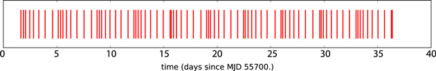
Figure 2. Times of the observations (offset from MJD 57700).
Download figure:
Standard image High-resolution imageA detailed account of the data processing and the source extraction is given in Paper I. Here we summarize the main data-reduction and processing steps. Basic calibrated data (BCD) are obtained from the Spitzer archive. Further data reduction is performed with the interactive data language (IDL) package cluster grinder (Gutermuth et al. 2009), which treats each BCD image for bright source artifacts. Aperture photometry is run on individual BCDs with an aperture radius of 24. To increase the signal-to-noise ratio and reject cosmic rays, the photometry from all BCDs in each visit is combined. The reported value is the average brightness of all the BCDs within the visit that contain the source in question, after rejecting outliers. The photometric uncertainties obtained from the aperture photometry are, particularly for bright sources, only lower limits to the total uncertainty, since distributed nebulosity is often found in star-forming regions and can contribute to the noise. To improve these estimates, Paper I introduces an error floor value that is added in quadrature to the uncertainties of the individual photometric points. The value of the error floor is 0.01 mag for [3.6] and 0.007 mag for [4.5].
Following Paper I, we retain all sources that have at least five data points in either [3.6] or [4.5]. We also require a detection to have been reported by Gutermuth et al. (2009). These requirements cut down on weak sources near strong ones that might be detected inconsistently. The latter led to the exclusion of 303 objects that had some measurements made. The bulk of these had [4.5] fainter than 15 and K fainter than 16. While four of these sources have Stetson indices in excess of our variability thresholds, they are impossible to verify because of their faintness and possible detector contributions to the variability signal. They are included in Table 1 for completeness. None had X-ray counterparts.
Table 1. Source Designations, Flux Densities, and Light Curve Properties of Sources That Were Rejected from Further Analysis for Being Relatively Faint and Hence Not Included in the Cryo Analysis
| ID | Name | Unit | Channel | Comment |
|---|---|---|---|---|
| 1 | RA | deg | ⋯ | J2000.0 R.A. |
| 2 | DEC | deg | ⋯ | J2000.0 Decl. |
| 3 | IAU_NAME | None | ⋯ | IAU designation within the YSOVAR program |
| 4 | UKIDSS_ID | None | ⋯ | UKIDSS designation |
| 5 | uKmag | mag | K | UKIDSS K-band mag. (1'' aperture) |
| 6 | e_uKmag | mag | K | Statistical error in uKmag |
| 7 | SEDclass | None | ⋯ | IR class according to SED slope |
| 8 | n_36 | ct | 3.6 μm | Number of data points |
| 9 | n_45 | ct | 4.5 μm | Number of data points |
| 10 | median_36 | mag | 3.6 μm | Median magnitude |
| 11 | median_45 | mag | 4.5 μm | Median magnitude |
| 12 | mean_36 | mag | 3.6 μm | Mean magnitude |
| 13 | mean_45 | mag | 4.5 μm | Mean magnitude |
| 14 | delta_36 | mag | 3.6 μm | Width of distribution from 10% to 90% |
| 15 | delta_45 | mag | 4.5 μm | Width of distribution from 10% to 90% |
| 16 | stetson_36_45 | None | 3.6–4.5 μm | Stetson index for a two-band light curve |
| 17 | redchi2tomean_36 | None | 3.6 μm | Reduced  to mean to mean |
| 18 | redchi2tomean_45 | None | 4.5 μm | Reduced  to mean to mean |
| 19 | coherence_time_36 | days | 3.6 μm | Decay time of ACF |
| 20 | coherence_time_45 | days | 4.5 μm | Decay time of ACF |
Only a portion of this table is shown here to demonstrate its form and content. A machine-readable version of the full table is available.
Download table as: DataTypeset image
We visually inspected all frames for light curves that are classified as variables in Section 3 and removed data points visibly affected by instrumental artifacts. Embedded star-forming cores like Serpens South pose significant problems for deriving accurate light curves with Spitzer/IRAC because of crowding issues, field rotation during the campaign causing column pull-down effects and scattered light effects to migrate over the cluster image, latent image effects, and pixel-phase effects. About 40 stars were removed outright, and another 65 sources had some data removed. We have done our best to provide good light curves by the design of our observations and by inspecting and cleaning all of the light curves discussed in this paper. However, some artifacts may remain that may, for example, influence some of the CMD slopes we derive. We believe that our conclusions are nevertheless robust to any remaining artifacts in the data.
The YSOVAR catalog starts with over 1800 sources detected at least five times in [3.6] or [4.5]. Of these, over 1500 have matches in observations from Gutermuth et al. (2009). These 1500+ sources are detailed in Table 2. Of these, 70 were detected in the MIPS 24 μm band. Nearly 1300 catalog sources have an additional K-band data point due to UKIDSS. About one-third of the monitored sources are in the middle field and were evaluated in both [3.6] and [4.5]. The remainder were either in the northern field, observed predominantly with [4.5], or the southern field, predominantly with [3.6] monitoring data. In the right part of Figure 1, we indicate the SED class of all YSOs in the monitored region. In the center of the field, there are about 30 YSOs, with the class Is outnumbering the class IIs. While the star-forming region appears most active in the central region, active star formation continues along the dust lane running from the northwest to southeast.
Table 2. Source Designations, Flux Densities, and Light Curve Properties of the Sources Used in This Study
| ID | Name | Unit | Channel | Comment |
|---|---|---|---|---|
| 1 | RA | deg | ⋯ | J2000.0 R.A. |
| 2 | DEC | deg | ⋯ | J2000.0 Decl. |
| 3 | IAU_NAME | None | ⋯ | IAU designation within the YSOVAR program |
| 4 | Colorclass | ⋯a | ⋯ | IR class according to color cuts |
| 5 | SEDclass | None | ⋯ | IR class according to SED slope |
| 6 | StandardSet | T/F | ⋯ | Source is in YSOVAR standard set |
| 7 | Augmented Set | T/F | ⋯ | Source is in YSOVAR augmented set |
| 8 | Variable | T/F | ⋯ | Source is variable |
| 9 | X-ray | T/F | ⋯ | An X-ray source |
| 10 | n_36 | ct | 3.6 μm | Number of data points |
| 11 | n_45 | ct | 4.5 μm | Number of data points |
| 12 | median_36 | mag | 3.6 μm | Median magnitude |
| 13 | median_45 | mag | 4.5 μm | Median magnitude |
| 14 | mean_36 | mag | 3.6 μm | Mean magnitude |
| 15 | mean_45 | mag | 4.5 μm | Mean magnitude |
| 16 | delta_36 | mag | 3.6 μm | Width of distribution from 10% to 90% |
| 17 | delta_45 | mag | 4.5 μm | Width of distribution from 10% to 90% |
| 18 | stetson_36_45 | None | 3.6–4.5 μm | Stetson index for a two-band light curve |
| 19 | redchi2tomean_36 | None | 3.6 μm | Reduced  to mean to mean |
| 20 | redchi2tomean_45 | None | 4.5 μm | Reduced  to mean to mean |
| 21 | period | days | ⋯ | Details in Table 2 |
| 22 | coherence_time_36 | days | 3.6 μm | Decay time of ACF |
| 23 | coherence_time_45 | days | 4.5 μm | Decay time of ACF |
| 24 | cmd_length_45_36 | mag | 3.6 μm, 4.5 μm | Length of the fitted CMD vector |
| 25 | cmd_angle_360 | degrees | 3.6 μm, 4.5 μm | Fitted CMD slope angle in degrees |
| 26 | cmd_angle_error_360 | degrees | 3.6 μm, 4.5 μm | 1σ error of fitted CMD slope angle |
| 27 | Jmag | mag | J | 2MASS J band magnitude |
| 28 | e_Jmag | mag | J | Statistical error in J mag |
| 29 | Hmag | mag | H | 2MASS H band magnitude |
| 30 | e_Hmag | mag | H | Statistical error in H mag |
| 31 | Kmag | mag | KS | 2MASS KS band magnitude |
| 32 | e_Kmag | mag | KS | Statistical error in Kmag |
| 33 | 3.6mag | mag | 3.6 μm | Cryogenic Spitzer/IRAC 3.6 μm band magnitude |
| 34 | e_3.6mag | mag | 3.6 μm | Statistical error in 3.6 mag |
| 35 | 4.5mag | mag | 4.5 μm | Cryogenic Spitzer/IRAC 4.5 μm band magnitude |
| 36 | e_4.5mag | mag | 4.5 μm | Statistical error in 4.5 mag |
| 37 | 5.8mag | mag | 5.8 μm | Cryogenic Spitzer/IRAC 5.8 μm band magnitude |
| 38 | e_5.8mag | mag | 5.8 μm | Statistical error in 5.8 mag |
| 39 | 8.0mag | mag | 8.0 μm | Cryogenic Spitzer/IRAC 8.0 μm band magnitude |
| 40 | e_8.0mag | mag | 8.0 μm | Statistical error in 8.0 mag |
| 41 | 24mag | mag | 24 μm | Cryogenic Spitzer/MIPS 24 μm band magnitude |
| 42 | e_24mag | mag | 24 μm | Statistical error in 24 mag |
| 43 | AK | mag | ⋯ | Extinction at K |
| 44 | uKmag | mag | K | UKIDSS K-band mag (1'' aperture) |
| 45 | e_uKmag | mag | K | Statistical error in uKmag |
| 46 | UKIDSS_ID | None | ⋯ | UKIDSS designation |
Note.
aClass 99 indicates disk-free; class −100 indicates unknown.Only a portion of this table is shown here to demonstrate its form and content. A machine-readable version of the full table is available.
Download table as: DataTypeset image
2.2. Matching to Other Catalogs
The YSOVAR data are cross-matched with data from the Chandra X-ray Observatory. The X-ray observation serves two purposes. First, since young stars are known to be relatively bright X-ray sources, the X-ray data provide a sample of cluster members independent of their IR characteristics, and therefore the X-ray data allow us to include diskless YSOs in the study. Second, we can test suggestions that X-ray activity is related to IR variability: both Wolk et al. (2015) and Poppenhaeger et al. (2015) found a weak trend that X-ray-detected cluster members vary on longer timescales than members undetected in X-rays.
Serpens South was observed by Chandra for 97.5 ks starting 2009 June 7. These data are being fully analyzed by E. Winston et al. (2017, in preparation). In total, they find 152 sources in the four chips of the ACIS-I array ( or 289'2 field of view). About 70'2 of the
  of the YSOVAR field is covered by the Chandra field. Only the southeast corner of the southern ([3.6] only) field is clipped (see Figure 1). Following the other YSOVAR papers, the matching radius is set to 1 arcsec, within 3' of the optical axis. To account for a slightly varying point-spread function, the matching radius was set to 2'', for sources more than 6' from the Chandra optical axis and 15 in between. This matching rule differs slightly from that used in Paper I and leads to the detection of seven additional sources. The net result was 37 X-ray sources were matched to sources (with five detections in the 82 IRAC visits) in the YSOVAR data.12
Near-IR data are taken from 2MASS (Skrutskie et al. 2006) and cross-matched by the cluster grinder pipeline (Gutermuth et al. 2009). Additionally, we take detections from the UKIRT Infrared Deep Sky Survey (UKIDSS) Galactic cluster survey, data release 9. The UKIDSS project is defined in Lawrence et al. (2007). UKIDSS uses the United Kingdom Infrared Telescope (UKIRT) Wide Field Camera (Casali et al. 2007) and a photometric system described in Hewett et al. (2006). The pipeline processing and science archive are described in Hambly et al. (2008). We only retain detections with a mergedClass flag between 3 and 0. Sources brighter than mK = 10 mag can be saturated, and we discard the UKIDSS data for any source that lies above this threshold. This leaves us with 2MASS data in the range KS = 5–16 mag and UKIDSS K = 10–17 mag. The luminosity function for both data sets is almost identical for K = 10–15. For fainter sources, 2MASS is incomplete; UKIDSS is incomplete for K > 17 mag. We chose not to include WISE data in the analysis due to source confusion in the core (i.e., the most interesting portion of the field).
2.3. Classification of IR Sources
The presence of an envelope or disk is sometimes described by the term "class." As originally proposed by Lada & Wilking (1984), "class" was based on the slope of the SED. The scheme modified by Greene et al. (1994) uses the shape of the mid-IR SED of candidate YSOs to sort them into different classes ranging from photospheric through stars with disks to those dominated by the infalling envelope. Several things complicate the identification of young stellar objects from infrared colors alone. First of all, galaxies with high rates of star formation can mimic the appearance of a single star with an envelope-like infrared excess. These galaxies tend to be fainter than most member stars. Second, circumstellar disks can generate differing levels of infrared excess. Depending on wavelength, face-on disks can appear redder than edge-on disks (Meyer et al. 1997), while disks with cleared centers or high accretion rates may exhibit larger excesses in the mid- and far-infrared as well. Finally, extinction along the line of sight can flatten the slope measured on the SED.
In Paper I, we defined a "standard set" of members for all tests so that direct comparison of results among the clusters studied in the YSOVAR project would be possible. The "standard set" of members includes all stars identified by Gutermuth et al. (2009) as color classes 0, 1, and 2 and transition disks.13 Because of the ambiguities in associating colors and disk class, Gutermuth et al. (2009) deredden sources before using a detailed system of magnitude and color cuts to identify sources as YSOs. This allows us to include several YSOs for consideration that have [3.6] > 15.
To be as inclusive and uniform as possible of YSOs in the field, especially when comparing between the clusters, we use the (nondereddened) slope of the SED from 2.2 to 24 μm, which can be measured for all members of the survey. Following Günther et al. (2014), we perform a least-squares fit and identify sources with  as class I,
  as flat spectrum (F), and
  as class II sources. Sources with
  are consistent with normal photospheres and hence are not suggestive of YSO status unless they are also X-ray sources. To account for these, we add to the set of "standard sources" X-ray sources that have SED slopes
  . For the purposes of determining the best possible slope, all of the available data including the UKIDSS measurements were used in these fits. While the UKIRT K-band data are included in the SED analysis, they are not in the color analysis as there is not a one-to-one correspondence with the 2MASS K filter, and hence they would break the uniformity across the study region we seek.
Our companion paper on Serpens South (E. Winston et al. 2017, in preparation) identifies YSOs in this region using the selection criteria outlined in Gutermuth et al. (2009). The procedure includes the removal of extragalactic contaminants and knots of PAH emission. Winston et al. did not include a search for deeply embedded YSOs, and so do not include three of the Gutermuth identified class 0 sources. Winston et al. further exclude six class 1 and eight class 2 sources that were below the magnitude cutoff at 3.6 μm for background contamination. These criteria were applied due to the wider field covered and the concurrent higher probability of background contamination away from the Serpens South core. These modest differences do not affect the discussion of derived results in a meaningful way.
As discussed in the previous papers of this series, coincidence between the SED-slope-based class and color-band class is very high, but not a one-to-one match. This leads to a gap in the definitions. Namely, the "standard set" is defined as the union of color-classed YSOs and X-ray sources with  . About 25% of the X-ray sources have
  but insufficient color information for a color class. Hence these are not part of the "standard set" but are still probably YSO cluster members. If they are brighter than mag 15 in [3.6] and [4.5], we identify these stars as the "augmented" set. There are six such objects and one additional X-ray object matched to a source fainter than [3.6] = 16. The lack of intervening sources indicates a clear gap between the augmented set and true background sources. In addition, it is clear that X-ray detection misses many, if not most, disk-free members of the cluster. For example, it is largely assumed that detections of exposed T Tauri stars in the Spitzer bands are complete. Only three of 17 class II sources (about 18%) are detected in X-rays. One-third of the 36 class 2 sources are detected in X-rays. So it is safe to suggest that the five class III sources identified represent between about one-fifth and one-third of the total.
Overall, Serpens South appears to be much younger and more embedded than the other YSOVAR clusters. The region also has a very dense dust lane running through it from northwest to southeast. This leads to strong reddening, which can skew the SED classifications. Despite this second point, there are very few cases in which the color class and slope class are highly discrepant. Of the 39 class 1 objects identified by Gutermuth et al. (2009), all but one are considered either flat spectrum or class I based on their SED. All of the class 0 sources identified using the Gutermuth et al. (2009) color techniques are found to be class I (the reddest slope designation) via the SED. Things are a little more muddled among the 36 other YSOs identified using colors (Gutermuth et al. 2009). Only 16 of these have intermediate negative (i.e., class II) slopes, and 14 are found to have shallow slopes, consistent with a class between 1 and 2 (i.e., flat SEDs).
2.4. The Mid-IR Cluster
Overall there were 1826 sources with at least five reliable detections in the 82 IRAC visits. Of those, 1524 were also identified in the cryo period data. These 1524 form the baseline set for further analysis. Ninety-nine of the 1524 were found to be variable, and 37 are X-ray sources.
While the cryo period data from this cluster were reduced in concert with the analysis reported by Gutermuth et al. (2009), a detailed analysis of the cluster itself was not undertaken at that time. The analysis done at the time included 423 stars in common with this sample. Of those, 43 were identified as class 0 or 1 and 36 as class 2 with one transition object. Figure 1 shows the YSO content of Serpens South. Overall, there are about 6400 individual sources in the full field depicted. We note in this image the deep dust lane running from the northwest to the southeast, mostly contained within the three fields monitored during the YSOVAR survey. Figure 3 shows the colors of the 85 YSOs in the standard set. This is broken down further as 44 with rising SEDs (class I sources), 19 flat SEDs, 17 class II SEDs, and five class III candidates. In addition to being the reddest, the class I and flat spectrum objects are by far the brightest population among the known members of this cluster: the average [3.6] = 12.3. This is a full magnitude brighter than the average class III object. There are multiple selection effects at play here. To be identified as a class I, we still require the object to have a YSO identification by Gutermuth et al. (2009), and this is only possible with detection in at least some of the 2MASS bands. Given the high extinction expected, this likely eliminates fainter class I sources from consideration. The X-ray sources also seem to be subject to strong selection effects, which seem to inhibit the detection of X-rays from sources fainter than about [3.6] ∼ 14. The net result is the typical X-ray source is almost 2 mag brighter than the non-X-ray-detected members of the standard set. There are also six X-ray-emitting stars identified with the augmented set.
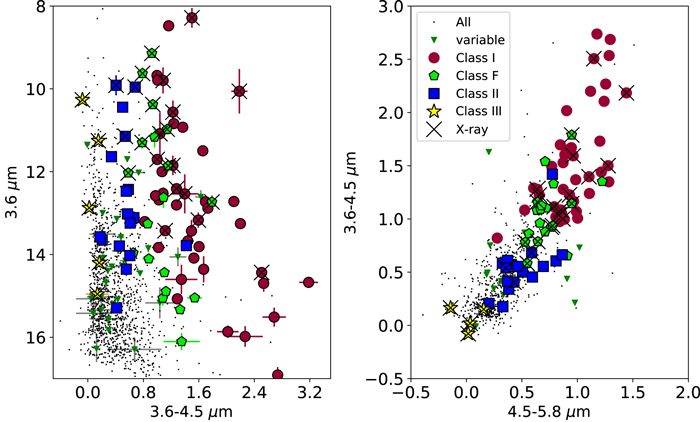
Figure 3. Left: a mid-IR color–magnitude diagram for the monitored sources in Serpens South. The extended lines from each source indicate the observed  and
and  values for each source. Right: a mid-IR two-color diagram for the same sources using the "cryo" period measurements. In both figures, the colors and shapes indicate the SED classes, while X indicates an X-ray source.
Download figure:
Standard image High-resolution imageFor the remainder of the paper, we will focus on the monitored fields. This is essentially a 5' by 5' box in the center of the field, plus the flanking fields, hereafter "[4.5]," "overlap," and "[3.6]" from north to south. There is a gap of about 1' separating the three fields, but only a few YSOs fall in these gaps. About half the YSOs identified by Gutermuth et al. (2009) are missed because they are completely outside the monitored field, including the grouping to the extreme southeast.
2.5. Variability
We ran several statistical tests on the distribution of the photometric data for each source. These were discussed exhaustively in Paper I and revisited by each of the YSOVAR papers (Günther et al. 2014; Poppenhaeger et al. 2015; Wolk et al. 2015), so we only quickly touch on key statistics below. For all sources, the mean and median magnitudes were calculated. We also calculated the median absolute deviation, the autocorrelation function (ACF), and the "Δ magnitude," which is the magnitude range between the 10% and 90% quantiles as initial (outlier resilient) variability measures.
To quantify variability, we calculated the reduced  to the mean of the magnitude for each of the bands. While very well understood in a statistical sense, this is not very sensitive to low-amplitude and symmetric variability. Instrumental uncertainties lead to a non-Gaussian error distribution, and we are forced to use a conservative cutoff to select variable sources (
 ; see Paper I). On the other hand, if the source is observed in both channels, the Stetson index is a more robust variability indicator (Stetson 1996). The Stetson index S is a fairly well known test for variability that is correlated in two or more channels. This is well discussed in the literature (e.g., Paper I; Carpenter et al. 2001; Rice et al. 2012; Günther et al. 2014). A larger value of the S index indicates larger coherent variability. The exact dividing line between variable and not variable requires careful analysis of each source, since the number of samples and errors on each observation enter into the precise determination. However, following Paper I, we consider sources with
  to be undoubtedly variable.
The Serpens South field has specific challenges for variability analysis. Almost 40% of the stars identified as candidate variables in our first pass were eventually rejected. One of the chief reasons for this was spurious variability due to the number of bright stars in the overlap field. This led to a larger than usual number of pulldowns and diffraction spikes. In some of these cases, we removed a block of data points or, when it was not clear which data were good and which data were contaminated, the entire light curve was excluded from analysis. In other cases, a single point was found to be nonphysically discrepant. In these latter cases, only the single point was excluded, but the net result was usually that the star was no longer identified as variable (usually due to the  becoming unremarkable).
Generally, variable YSOs trace out a trajectory that is often linear in the near-IR (Carpenter et al. 2001; Rice et al. 2012). In the previous papers of this series, we have found that the points occupied by the individual observations of a single star can be fitted to a slope that is well defined in the [3.6] versus [3.6]–[4.5] color–magnitude diagram (CMD). For each source, we fitted a straight line to all points in the CMD using an orthogonal distance regression method that takes the errors in both the color and magnitude into account. This allows us to compare, in a quantifiable way, the trajectories that variable YSOs follow in color–magnitude space. We will discuss the results and meaning of these fits in detail in Section 4.4.
2.6. Period Searches
Following Paper I, we performed a period search on all light curves with at least 20 points. We computed results using several methods: Lomb–Scargle (LS; Scargle 1982), box-fitting least squares (Kovács et al. 2002), and Plavchan (Plavchan et al. 2008), as well as the ACF on the 3.6, 4.5 μm, and, where possible, the [3.6]–[4.5] light curves. Given the overall sampling of our data, we only allow period detections on timescales consistent with at least two and a half periods being observed over the window of the collective YSOVAR observations: that is, we were sensitive to periods between 0.1 and 14.5 days. Typically, if the LS algorithm found a reliable period, the other approaches found comparable periods, and this period was used. If the results were inconsistent, no period is given.
We excluded candidate periodic objects if the calculated false alarm probability (FAP) was >0.03. For each of the remaining objects, we investigated the phased light curve. In priority order, we take any period derived from the [3.6] data first ([3.6] is less noisy than [4.5]); then, only if there is no [3.6] period of sufficient power, we take the period derived from [4.5]. We also derived a period from the [3.6]−[4.5] color. Only two periods were identified using color, and both concurred with previously identified cycles.
The formal errors on the period determination with linear frequencies are very small when there are 82 samples spaced over 38 days, about 0.0007 (in frequency space) for a 3σ signal (e.g., Equation 14 in Horne & Baliunas 1986). Hence, the precision is a function of both the period and amplitude of each star. But assuming a 3σ signal, typical periods should be precise to better than 0.001 days for periods below a day, 0.01 days for periods below 4 days, and 0.04 days for periods below 7 days, and periods of 14.5 days should have a precision of about 0.15 days. One caveat is that some of the periods are more stable than others. This appears in the periodogram analysis as either a wider peak or a higher FAP. However, sources in Table 3 with higher FAPs have a correspondingly greater uncertainty in their periods. Further, the periods are measured by tracing ephemeral phenomena (such as spots and disk warps), so phase shifts are common among YSOs and limit the ultimate precision of such a period determination. In Table 3, we list the periods to two decimal places, with the exception of one object that has a period of less than 1 day and appears to be an eclipsing binary.
Table 3. Properties of Periodic Sources
| IAU Name | X-ray | Standard set | Period | Per. | False | Peak | Classa from | Class from | Period |
|---|---|---|---|---|---|---|---|---|---|
| source | of cluster | Δ | alarm | Gutermuth | SED | fromb | |||
| SSTYSV_J... | members | [days] | [days] | prob. | [power] | et al. (2009) | slope | [filter] | |
| 182955.44−020245.6 | No | No | 9.26 | ⋯ | 0.010 | 13.59 | −100 | II | 45 |
| 182957.07−015946.0 | No | Yes | 5.92 | ⋯ | 0.039 | 11.49 | 2 | I | 45 |
| 182957.54−020430.2 | No | No | 0.12 | ⋯ | 0.017 | 13.10 | −100 | II | 45 |
| 182958.60−020321.0 | No | No | 8.86 | 0.4 | 0.011 | 13.49 | −100 | II | 36/45 |
| 182958.79−020004.0 | No | Yes | 13.52 | 0.43 | 0.000 | 22.32 | 2 | I | 36/45 |
| 182958.86−020245.7 | No | No | 12.31 | ⋯ | 0.007 | 14.01 | 99 | III | 45 |
| 182959.02−020157.4 | No | Yes | 13.98 | 1.02 | 0.019 | 12.97 | 1 | I | 36/45 |
| 182959.47−020106.4 | Yes | Yes | 11.95 | 0 | 0.002 | 15.18 | 1 | I | 36/45 |
| 182959.89−020335.3 | No | Yes | 12.69 | ⋯ | 0.028 | 12.56 | 2 | F | 36 |
| 183000.22−020052.5 | No | Yes | 13.52 | 0 | 0.027 | 12.60 | 1 | I | 36/45 |
| 183000.26−020015.5 | No | Yes | 6.01 | 0 | 0.001 | 15.97 | 1 | I | 36/45 |
| 183000.56−020211.4 | Yes | Yes | 5.6 | 0.08 | 0.003 | 14.97 | 1 | I | 36/45/clr |
| 183001.26−020148.3 | No | Yes | 10.43 | 0 | 0.061 | 11.78 | 1 | I | 36/45 |
| 183002.44−020257.9 | Yes | Yes | 7.42 | 0.14 | 0.000 | 16.92 | 1 | I | 36/45 |
| 183002.47−020304.3 | No | Yes | 7.7 | 0.14 | 0.003 | 14.72 | 1 | I | 36/45 |
| 183003.01−021110.7 | Yes | No | 3.01 | ⋯ | 0.004 | 14.32 | 99 | II | 45 |
| 183004.04−020123.4 | Yes | Yes | 5.68 | ⋯ | 0.005 | 14.31 | 2 | F | color |
| 183005.15−020104.4 | No | Yes | 4.82 | ⋯ | 0.001 | 15.76 | 99 | II | 36 |
| 183005.23−020206.5 | Yes | Yes | 8.86 | ⋯ | 0.004 | 14.66 | 2 | I | 36 |
| 183006.20−020219.6 | Yes | Yes | 11.95 | −0.34 | 0.023 | 12.77 | 2 | II | 36/45 |
| 183006.72−020319.0 | No | No | 0.12 | 0 | 0.000 | 21.44 | −100 | II | 36/45/clr |
| 183006.93−015631.6 | Yes | Yes | 5.53 | ⋯ | 0.025 | 12.67 | 2 | II | 36 |
| 183009.65−020801.8 | No | No | 0.18 | ⋯ | 0.001 | 16.13 | −100 | II | 45 |
| 183010.80−020354.6 | Yes | Yes | 6.92 | ⋯ | 0.001 | 15.60 | 2 | I | 36/45 |
| 183011.21−020420.1 | No | No | 0.22 | ⋯ | 0.000 | 18.87 | −100 | F | 45 |
| 183012.13−020231.1 | No | No | 10.47 | ⋯ | 0.024 | 12.66 | −100 | II | 45 |
| 183013.75−020245.8 | No | No | 13.03 | 0.49 | 0.000 | 25.90 | −100 | II | 36/45 |
| 183013.94−020205.5 | No | No | 8.45 | ⋯ | 0.011 | 13.50 | −100 | II | 45 |
| 183014.63−020242.9 | No | No | 12.51 | ⋯ | 0.002 | 14.58 | −100 | II | 45 |
| 183016.24−020928.7 | No | Yes | 12.51 | ⋯ | 0.001 | 15.57 | 2 | I | 45 |
| 183016.46−021023.7 | No | No | 12.23 | ⋯ | 0.030 | 12.28 | −100 | I | 45 |
| 183016.60−021049.9 | No | No | 10.62 | ⋯ | 0.011 | 13.15 | −100 | II | 45 |
Notes.
aClass 99 indicates disk-free; class −100 indicates unknown. bFilter used for the period value in column 4 is in bold.Download table as: ASCIITypeset image
3. Results
3.1. Periodic Sources
Overall, 32 of the 1524 sources showed significant periods between 0.1 and 14.5 days. These are split between 18 from the standard set of cluster members and 14 other stars. Among the nonstandard set sources, four have subday periods, suggestive that they are likely to be tidally locked binaries. One of these, 183003.01−021110.7 (period of ∼3 days), is a member of the augmented set of cluster members, that is, a star we think is a cluster member but that does not meet all of the criteria for the YSOVAR standard set (see Section 4.2). The remaining 28 periodic stars range in period from about 8.5 to 13 days with no obvious distinction between those in the standard set and those outside the standard set.
In Table 3, we list the properties of the periodic sources. In addition to the star name and the period, we include the FAP and the power of the periodogram. We also include the color class as determined by Gutermuth et al. (2009) and the 2–24 μm SED slope class for comparison. We also track which periodic sources are X-ray sources and which are part of the standard set of cluster members based on the definition in Section 2.
From this we can see that four periodic sources had insufficient data for color classification; this acts as a reminder that every source gets an SED slope classification, but only 65% in this sample have the same classification in both systems. This is consistent with Paper I, which systematically compared results between color and SED classes and found three-quarters of the objects received the same classification (i.e., class 2 and class II) using both color- and SED-based methods. The slope classification, which we use throughout the analysis, cannot distinguish transition objects from class II when using the 2–24 μm slope. Two of the periodic YSOs are identified as transition objects by Gutermuth et al. (2009).
Figure 4 shows the cleanest periodic light curve. With a period of about 2.808 hr, this appears to be a contact binary. The period is stable over the 40 days of observations and is measured to a precision of 3 minutes. The reddening seen as a function of phase is shallower than that expected due to ISM dust reddening and is more likely due to the smaller eclipsing body being cooler than the primary. Figure 5 shows two examples of quasi-periodic light curves among our sample, similar to what is often seen for classical T Tauri stars (Cody et al. 2014). The class I object SSTYSV J183000.56−020211.4 has a ∼5.6 day period that is visually obvious, with a typical peak-to-trough change of about 30%. There are tantalizing hints at the end of the monitoring period that the downward trend is embedded in a larger cycle: the fifth peak is more than 30% below the first peak. The ∼6 day period of the class I SSTYSV J183000.26−020015 is similarly clear on inspection. While there is no linear trend, the cycle-to-cycle variations are significant, and the fifth trough seems to be absent. Both objects redden (middle panel of the figures) exactly as expected due to ISM reddening.
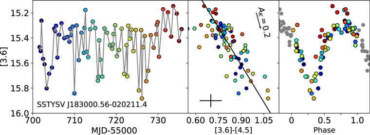
Figure 4. Light curve for object SSTYSV J183006.72−020319.0. In the left panel, we show the raw light curve for [3.6]. In the center panel, we plot the [3.6]–[4.5] color against the [3.6] magnitude for the source. The solid line is a fit to the data with a slope of about 82° ± 3°. The arrow indicates an AK = 0.2 reddening vector, adapted from Indebetouw et al. (2005), and the typical errors are indicated near the bottom. The data folded on the 0.12 day period is shown in the right panel. The colors of the dots change with time, from blue at early time to red at late time. In the phased panel, more than one full phase is shown for clarity, and the repetitive data are shown as gray.
Download figure:
Standard image High-resolution image
Figure 5. Top: light curve for the class I object SSTYSV J183000.56−020211.4. Bottom: the class I SSTYSV J183000.26−020015. Symbols and panel descriptions are the same as in the previous figure. The folded data do not overlap exactly. In the case of SSTYSV J183000.56−020211.4, it appears a long-term cycle may be superimposed. In both cases, the color variances are consistent with changes in reddening.
Download figure:
Standard image High-resolution imageAs mentioned above, the discrete ACF of each light curve is calculated. The ACF can be thought of as a coherence time, the time it takes for the signal to diverge from the original and then return to the starting phase. If a star has a purely periodic nature, the ACF will have a peak at the periodic frequency with a minimum at one-half the period when the evaluated signal and the original signal are out of phase. The ACF is statistically well defined for evenly sampled data. While this is unevenly sampled data, we have discussed the physical interpretation of this in the previous papers of the series. Following Günther et al. (2014), we take the first value of τ with ACF(τ) < 0.25 as the coherence time for the light curve.14 The values of the periods of the periodic sources in Serpens South and the ACF appear linearly correlated. Specifically, using a linear regression, we find the coherence time is about 25% of the period. The best fit is offset from zero, and the period is related to the coherence time as period = 0.15 × coherence time + 0.7. This is very close to what was found for GGD 12–15 and a similar result for IRAS 20050+2720 (Poppenhaeger et al. 2015; Wolk et al. 2015). Numerical analysis also yields similar results (Findeisen et al. 2015). Even though this trend has now been shown to be consistent over about 100 periodic sources, we do not mean to imply the coherence time gives us the absolute timescale of the physical processes at work. Instead, it provides for a relative comparison of long versus short timescales for changes in the nonperiodic YSOs.
3.2. Variable Sources: Nonperiodic
The total number of variables according to all criteria is 99. This includes 58 of the 85 stars from the standard set of cluster members. Among the standard set of members, 68% ± 5% are variable.15 Figure 6 shows the observed variability of the individual sources. The standard set includes 28 X-ray sources, of which 23 (82% ± 8%) are variable. This is only slightly higher than the variability among the general population of flat SED and class I sources, 48 of 63 (76% ± 5%). The class II sources are slightly less likely to be detected as variable: 10 of 17 (59% ± 12%). Similar results are found for class 0 or 1 sources as for class I and flat spectrum with variability levels around 75%. Class 2 sources also have variability rates around 75%, which is sufficiently different from the class II result to indicate at least some contamination of non-disk-bearing stars among the class II subset. On the other hand, none of the X-ray sources with class III SEDs are variable (Table 4). So there is no evidence here that X-ray sources are more IR variable than the general population of YSOs.
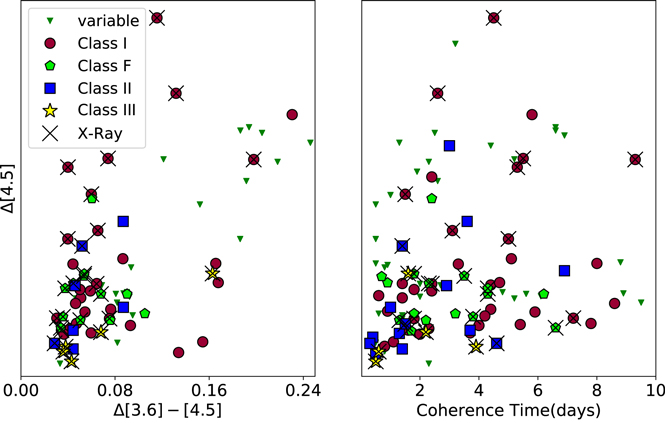
Figure 6. Scatter plots of the key IR parameters for variable sources. In all plots, blue squares indicate class II objects, gold stars indicate X-ray sources with SED slopes appropriate for photospheric SEDs, and the red hexagons and circles are objects with flat spectrum or class I SEDs, respectively. X-ray sources and variables not in the standard set are identified by X and green downward triangles, respectively. The Y axis in both plots is the range of change of values at [4.5] with the upper and lower 10% of the data points removed. The X axis of the left-hand plot is the change in the [3.6]–[4.5] values with the 10% outliers removed. Very few sources show extreme color changes, but those that do are likely to be class I or variables that are not in the standard set. The X axis in the right-hand plot is the "coherence time" for the [4.5] light curves (i.e., the value of τ when the ACF(τ) = 0.25). The class III sources have the shortest coherence time. The longest coherence times are possessed by class I sources.
Download figure:
Standard image High-resolution image
Figure 7. Amplitude of variability of light curves of variables (90th minus 10th percentile in mag) in [3.6] and [4.5]. The amplitudes are similar for SED classes I, F, and II, but significantly smaller for SED class III and higher for the variables not matched to the standard set. The spread in flux of individual member star light curves tends to be larger in [3.6] than in [4.5].
Download figure:
Standard image High-resolution imageTable 4. Variability Metrics for Subsamples
| Subset | Number | # Vars. | % |
 [med.]a [med.]a
|
 [med.]a [med.]a
|
S[med.]a |
|---|---|---|---|---|---|---|
| [avg.] | [avg.] | [avg.] | ||||
| Standard | 85 | 58 | 68 | 0.13 | 0.12 | 2.83 |
| set | 0.17 | 0.15 | 3.73 | |||
| Class I | 44 | 34 | 77 | 0.14 | 0.13 | 2.95 |
| 0.21 | 0.17 | 4.25 | ||||
| Class F | 19 | 14 | 74 | 0.13 | 0.11 | 3.43 |
| 0.13 | 0.11 | 3.12 | ||||
| Class II | 17 | 10 | 59 | 0.12 | 0.11 | 2.46 |
| 0.13 | 0.13 | 2.35 | ||||
| Class III | 5 | 0 | 0 | ... | ... | ... |
| Class 0/1 | 43 | 29 | 72 | 0.17 | 0.12 | 3.08 |
| 0.22 | 0.18 | 4.84 | ||||
| Class 2 | 36 | 28 | 78 | 0.12 | 0.12 | 2.40 |
| 0.14 | 0.12 | 3.04 | ||||
| Augmented | 50 | 37 | 74 | 0.17 | 0.14 | 2.77 |
| class I | 0.19 | 0.19 | 4.61 | |||
| Augmented | 19 | 11 | 58 | 0.14 | 0.13 | 3.36 |
| class II | 0.14 | 0.14 | 4.06 | |||
| X-ray only | 28 | 23 | 82 | 0.14 | 0.12 | 3.95 |
| 0.20 | 0.17 | 4.81 | ||||
| All others | 1429 | 37 | 3 | 0.16 | 0.15 | 0.97 |
| 0.17 | 0.20 | 1.10 | ||||
Note.
aThese columns list two metrics for the measured quantities (Δ[3.6], Δ[4.5], and Stetson index, respectively). The top value is the median of all the variables of the given subset. The bottom value is the average value of all the variables of a given subset.Download table as: ASCIITypeset image
We examined the distribution of color change and coherence time as a function of magnitude change for the various classes. Figure 6 shows the class III variables have the smallest change: typically ![${\rm{\Delta }}([3.6]\mbox{--}[4.5])\lt 0.05$](https://content.cld.iop.org/journals/1538-3881/155/2/99/revision1/ajaaa6c4ieqn25.gif) . The other classes show a lot of overlap, but the class I and flat spectrum sources seem the most likely to have large, slow changes. The latter is quantified as high values of coherence time. For class I sources, the median coherence time is about 3.5 days, almost a day longer than flat spectrum objects (∼2.75 days) and nearly double that of the class IIs (about 2 days) and triple the median coherence time of the class IIIs (about 1 day). In all cases, the coherence time is longer in [4.5] than in [3.6]. An Anderson–Darling test (Anderson & Darling 1952) confirms the coherence times for the class II and class I/F variables are not drawn from the same parent population, further confirming the timescales for mid-IR variability are longer for the more embedded classes of YSOs. Meanwhile, the distributions of the class I and flat spectrum sources are indistinguishable and often have coherence time in excess of 4 days. Following the reasoning in the previous section—wherein we found coherence time was about one-fifth of the period—if these stars are periodic and have coherence time ≥3 days, the observation window would have been too short to identify the periodic nature of most of the class I objects. There are also trends of larger variability and larger color changes with steeper SEDs. Most color changes are
. The other classes show a lot of overlap, but the class I and flat spectrum sources seem the most likely to have large, slow changes. The latter is quantified as high values of coherence time. For class I sources, the median coherence time is about 3.5 days, almost a day longer than flat spectrum objects (∼2.75 days) and nearly double that of the class IIs (about 2 days) and triple the median coherence time of the class IIIs (about 1 day). In all cases, the coherence time is longer in [4.5] than in [3.6]. An Anderson–Darling test (Anderson & Darling 1952) confirms the coherence times for the class II and class I/F variables are not drawn from the same parent population, further confirming the timescales for mid-IR variability are longer for the more embedded classes of YSOs. Meanwhile, the distributions of the class I and flat spectrum sources are indistinguishable and often have coherence time in excess of 4 days. Following the reasoning in the previous section—wherein we found coherence time was about one-fifth of the period—if these stars are periodic and have coherence time ≥3 days, the observation window would have been too short to identify the periodic nature of most of the class I objects. There are also trends of larger variability and larger color changes with steeper SEDs. Most color changes are  mag. Only nine stars in the standard set exceed this, but eight are class I. Class I sources also account for all seven standard set objects with
  mag.
mag.
Qualitatively there is little difference in the view presented by analyzing the sources based on color or slope. Neither is more informative on the main point: the disked or otherwise embedded stars are more likely to be variable than those without disks.
The variable sources are strongly concentrated in the central field, thought to be the core of Serpens South. There are significantly fewer sources in the [3.6] and [4.5] overlap field compared to the adjacent fields. There are 343 sources in the central field and over 550 in each of the fields dominated by one-color data. Much of this is due to the dust lane visible in Figure 1, combined with the preponderance of bright stars in the core, which overwhelm the nearby sources. Nonetheless, the variables are strongly concentrated in the core, with 66 of them in the central region. Conversely, while there are 558 sources in the [4.5]-only footprint, only 20 are variables via the  or periodic metrics (3.5%). Nine of those variables are among the 16 standard set members in the [4.5]-only footprint. Similarly, while there are 623 sources in the [3.6]-only footprint, only 14 of those are variables. Seven of the [3.6]-only variables are among the 10 standard set members in that footprint.
4. Discussion
4.1. Variability and Class
As in the previous papers in this series, we characterize the amplitude of variability in a given light curve by the spread of the individual magnitudes. To account for possible outlying data points in the light curves, we report "Δ," which is the range from the 90th percentile to the 10th percentile in magnitude. In Table 4, we list the basic metrics of variability. The first column lists the subset of interest. The second column indicates the number of sources of each subset. The third column lists the number of variables as determined either by periodicity, the reduced  test, or the Stetson test. The remaining columns list statistics of the variable sources in the field using the values of Δ [Channel]. This is the width of the distribution of photometric measurements for each source from 10% to 90%, so it excludes outliers, including flares and eclipses. The final column indicates the median/average Stetson index.
The fractions of class I and flat spectrum objects (and class 0/1 and class 2) found to be variable are nearly identical. As seen in Table 4, class II variability rates are slightly lower. The variability metrics measured in GGD 12–15, IRAS 20050+2720, and Mon R2 have class II variability rates more or less consistent with class I and flat spectrum sources. On the other hand, NGC 1333 and L1688 both indicate a variability rate of class IIs of about 60%, in line with what is found here. In fact, the class-by-class variability rates found in Serpens South are nearly identical to the results found in NGC 1333 (Rebull et al. 2015). The data here also match the general trend for L1688, where it was noted that the more positive the slope, the higher the variability rate, but the effect is small (Günther et al. 2014).
The results in Table 4, broken down by SED class, are shown in Figure 7. We find that sources with IR excesses, that is, SED classes I, F, and II, show mean 3.6 μm variability amplitudes of about 0.13. The distribution of amplitudes is broad and reaches ∼0.5 mag for disk-bearing sources. In contrast, diskless stars, that is, objects with SED class III (typically assumed to have no disk), show a markedly different pattern. They are found to have little variability (mean amplitude ∼0.05 mag at 3.6 μm), and none is identified as variable.
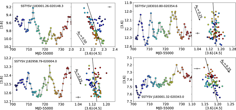
Figure 8. Four of the five most variable stars as determined by S index. SSTYSV J183010.80−020354.6 and SSTYSV J182958.79−020004.0, both class 2 objects, show cyclic behavior. The class 1 objects, SSTYSV J183001.26−020148.3 and SSTYSV J183001.32−020343.0, show steadier changes. None of the four shows a strong color change, despite the large amplitude changes.
Download figure:
Standard image High-resolution imageTwo examples of variables are shown in Figure 9. Both of these are class I objects. The first, SSTYSV J183005.77−020158.1, decreases in brightness constantly during the observation period, experiencing a total change of 0.5 mag at [3.6]. Meanwhile, the second, SSTYSV J183004.39−020138.2, changes by about 0.15 mag (peak to trough). In addition to the long-term trend, both show significant short-term changes. Typically, changes in [3.6] are larger than in [4.5].
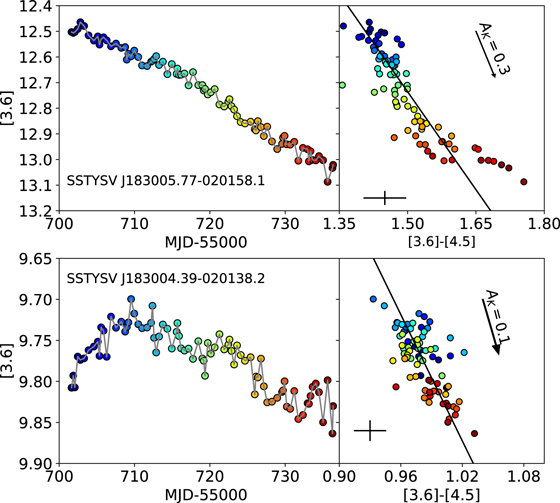
Figure 9. Light curves for the class I objects SSTYSV J183005.77−020158.1 (top) and SSTYSV J183004.39−020138.2 (bottom). In the left panels, we show the raw light curve for [3.6]. In the right panels, we plot the [3.6]–[4.5] color against the [3.6] magnitude for the source. The solid line is a fit to the data. In both cases the slope is about 69°. The arrow indicates the reddening vector, adapted from Indebetouw et al. (2005), which also has a slope of about 74°. The typical errors are indicated near the bottom of the right-hand figures.
Download figure:
Standard image High-resolution imageTo test if distributions of amplitude and color changes for each SED are drawn from the same parent distribution, we use the Anderson–Darling two-sample test. We test each combination of SED classes. One-to-one, there is not a significant difference in the Δ values for [3.6] and [4.5]. The Anderson–Darling test does not conclusively demonstrate the samples are drawn from different parent populations. However, there is a trend that class I sources show larger Δ values than the YSOs with more negative slopes. While the class III sources clearly stand apart, the small number of disk-free members identified in this cluster makes distinctions challenging (Figure 7). Despite the small numbers, the Anderson–Darling test does reach 99% confidence that the class III amplitudes are different than the other classes, but only at [3.6] (Table 5).
Figure 10 shows one of the most interesting YSO variables we have found. SSTYSV J183006.13−020108.0 is identified as class I by both color and SED that varied by over 50%. This is one of the most variable objects observed. The light curve could be periodic with a period of about 35 days, but only one "cycle" was observed. The color also appears cyclic with a color change of about 0.3, roughly oriented along the reddening vector. This is reminiscent of the light curve of the class II object ISO-Oph 140 (Günther et al. 2014), which showed a very similar cycle over a 30 day period, albeit with a color change of about 0.1 and a brightness change of about 0.25 in that case.
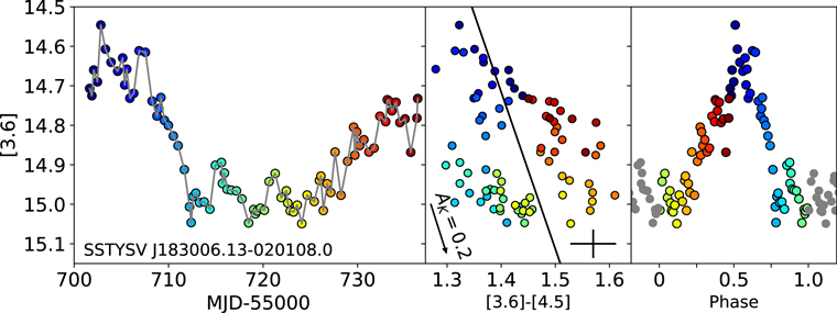
Figure 10. Light curves for the class I SSTYSV J183006.13−020108.0. This is a class I object with a slow, smooth, possibly periodic, change. A 35 day period was determined by inspection. The color change also appears cyclic. There are a few other such examples noted in the YSOVAR data set (see, e.g., Günther et al. 2014).
Download figure:
Standard image High-resolution imageTable 5. Anderson–Darling p Values for Variability Amplitudes across Class; Significant Differences Bold-faced; See Text for Details
| Δ[3.6] | Class F | Class II | Class III |
|---|---|---|---|
| Class I | 0.53 | 0.10 | 0.00 |
| Class F | ⋯ | 0.17 | 0.01 |
| Class II | ⋯ | ⋯ | 0.01 |
| Δ[4.5] | |||
| Class I | 0.40 | 0.13 | 0.02 |
| Class F | ⋯ | 0.08 | 0.02 |
| Class II | ⋯ | ⋯ | 0.22 |
| Δ[3.6] | Class 0 | Class 1 | |
| Class 1 | 0.25 | ⋯ | ⋯ |
| Class 2 | 0.13 | 0.29 | ⋯ |
| Δ[4.5] | ⋯ | ⋯ | ⋯ |
| Class 1 | 0.41 | ⋯ | ⋯ |
| Class 2 | 0.33 | 0.50 | ⋯ |
Download table as: ASCIITypeset image
Establishing the "most variable object" is not entirely straightforward because, for example, the most variable in 3.6 might not be the most variable at [4.5], and the standard deviation and Δ metrics give results that differ slightly, which can lead to a different rank order. Further, various forms of noise contribute to the variability of fainter sources. Confining ourselves to the Stetson index gave reasonably consistent results without bias to faint sources, which could be noise dominated. The overall performance of the Stetson index with regard to well-sampled Spitzer data is discussed in Cody et al. (2014). Among our total sample of 1524 sources, 343 were sampled in both colors often enough to obtain Stetson indices. Eight sources had  . Of these, three-quarters of those were class I (or class 1). In Table 6 we list those eight sources to look for additional trends. Four of these are plotted in Figure 8. There does not seem to be a luminosity bias as the sources range in [3.6] from about 7.5 to nearly 13.75. Nearly all of these highly variable sources have colorless brightness changes. The trajectory the object makes in the CMD is within 10° of vertical in all but one case. The only object that shows changes consistent with reddening is SSTYSV J183000.56−020211.4, which is a periodic class I object that shows signs of long-term reddening changes (Figure 5).
Table 6.
Properties of the Eight Stars with Stetson Index 
| IAU Name | Color | SED | Median | Δ | Δ | S | CMD | Angle | |
|---|---|---|---|---|---|---|---|---|---|
| class | class | [3.6] | [4.5] | [3.6] | [4.5] | angle | err | ||
| SSTYSV J183001.26−020148.3 | 1 | I | 9.76 | 7.54 | 0.54 | 0.48 | 15.54 | 83.24 | 1.10 |
| SSTYSV J183000.56−020211.4 | 1 | I | 11.23 | 10.10 | 0.51 | 0.38 | 14.37 | 75.54 | 0.43 |
| SSTYSV J183010.80−020354.6 | 2 | I | 12.24 | 11.08 | 0.23 | 0.24 | 7.73 | 87.53 | 3.31 |
| SSTYSV J182958.79−020004.0 | 2 | F | 12.50 | 11.38 | 0.25 | 0.24 | 7.67 | 87.09 | 2.02 |
| SSTYSV J183001.32−020343.0 | 1 | I | 7.43 | 6.26 | 0.24 | 0.18 | 7.32 | 85.50 | 1.25 |
| SSTYSV J183005.17−020141.5 | 1 | I | 10.20 | 8.96 | 0.32 | 0.29 | 6.70 | 83.44 | 1.05 |
| SSTYSV J183002.27−020159.3 | 1 | I | 10.55 | 9.22 | 0.28 | 0.28 | 6.67 | 88.87 | 4.18 |
| SSTYSV J182959.47−020106.4 | 1 | II | 13.73 | 12.17 | 0.18 | 0.19 | 5.42 | 95.99 | 2.15 |
Download table as: ASCIITypeset image
4.2. The Augmented Set
The augmented set is composed of X-ray sources that are brighter than 15 mag in either [3.6] or [4.5] and that have SED slopes consistent with class I, F, or II objects, but the colors of these objects are not sufficient for positive identification as YSOs. There are eight such objects. There are only three other X-ray sources that matched Spitzer sources, and all are fainter than [3.6] = 16. So there appears to be a clear gap between the augmented set with [3.6] brighter than 15 and true background sources with [3.6] > 16.
Four of the augmented-set stars are variable. Three of these have rising class I SEDs and show long and slow changes of about 20%, very much in line with standard-set class I objects. The fourth, SSTYSV J183003.01−021110.7, was only monitored at [4.5]. This star has a 3 day period and peak–trough changes of less than 8%.
4.3. Variables Not in the Standard or Augmented Sets
There are 37 variables among stars not in the standard or augmented sets. This represents about 30% of the variables, but less than 3% of the monitored field stars. These stars tend to be fainter than those in the standard set of cluster objects. Variables in the standard set of cluster objects have a mean [4.5] ∼ 11, while these have a mean [4.5] ∼ 13.75. Of the 37, 13 are periodic (see Figure 11 for two examples). This subgroup includes four stars with periods of less than 6 hr, which are probably tidally locked binaries. The other nine periodic stars all have periods between 8 and 13 days. Only two of the periodic sources (one short period, one longer period) were noted to be intrinsically variable via the Stetson or  tests, so the periodic sources tend to be weak variables. The weak signals in the stars with periods of 8–13 days suggest that some of these objects may be spotted, disk-free, young stars, that is, possible class III objects. In addition to their relatively low absolute variability, the periodic sources in the long-period (8–13 day) subgroup have relatively low reddening (
 ). The mean reddening for the other variables in the nonstandard set is AK = 1.2, which while significant is not as large as for the typical star in the standard set.
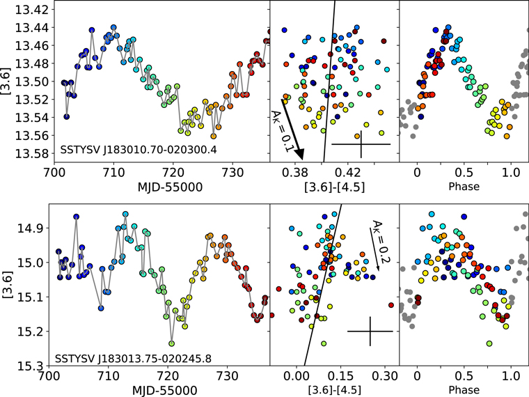
Figure 11. Top: SSTYSV J183010.70−020300.4 is not detected in the J and H bands; its SED is consistent with a class II object. The star may be periodic on a 25 day timescale, but less than 1.5 cycles are observed. No color change is detected. Bottom: SSTYSV J183013.75−020245.8, another very red object with a class II SED. The period is very clear (especially in the spacing of the peaks), but the star gets bluer when it is fainter. This is one of the cleanest examples of "bluing" in this cluster.
Download figure:
Standard image High-resolution imageThe periodic and nonperiodic variables represent different samples of stars. The amplitude of the changes in variables that are not in the standard (or augmented) set is higher than for variables that are in those sets. This is undoubtably a selection bias; a larger-amplitude variability is needed by our algorithms if the variability is not periodic. This occurs because the variables not in the standard or augmented sets are fainter than the standard-set stars. Further, in these stars, the change in [4.5] tends to exceed the change in [3.6]. We were originally suspicious these could be false positives induced by background noise. We checked each of these sources by eye, but only one variability candidate was removed for obvious contamination. Figure 12 shows an example of one source that appears to show real variations. The noise per sample appears to be about 5%, but the trend is clear and consistent with reddening.

Figure 12. Top: SSTYSV J183005.33−020111.8 appears deeply to be an embedded source. It was not detected by 2MASS in the J or H bands, so the procedure of Gutermuth et al. (2009) could not classify the source. Thus, it is not in the standard set of cluster members. In the IRAC bands, the source has a rising SED and brightens monotonically for about a month. The changes are consistent with a decrease in reddening of about  . Bottom: SSTYSV J183005.81−020205.8 is another example of a highly reddened star not detected in 2MASS J or H and thus is not in the standard set of cluster members. However, this star is bluer when it is fainter.
Download figure:
Standard image High-resolution image4.4. Color Changes
As has been discussed in the previous papers of this series, the additional dimension of color information comes into play for sources with both [3.6] and [4.5] data available. Previous YSOVAR papers have shown the influence of cool spots, hot spots, dust absorption, and accretion (following Espaillat et al. 2010) on the [3.6] versus [3.6]–[4.5] CMD. To investigate the dependence of CMD slopes on SED class, we performed linear fits to the CMDs of all variable sources in our standard set. The data points in the CMDs have nonnegligible errors in both the magnitude and color directions. To take these errors into account simultaneously, we performed a least-squares orthogonal fit to a straight line, using the Python package scipy.odr, which performs an orthogonal distance regression with a Levenberg–Marquardt-type algorithm. We define our slope angles as the clockwise angle from a horizontal line. Figures 9–11 give examples of some of the fits. We show all fitted CMD slopes as a function of SED class in Figure 13, together with the length of the vectors spanned in the CMD. We have omitted sources with fitted slopes that have very large errors (>10%); typical errors are below 5°. The expected angular slopes for standard (ISM) reddening, cool and hot spots, are indicated on the plot as well (76° for ISM reddening, ∼85° for cool spots). Angles >90° are generally attributed to other processes such as accretion or scattered light (Kesseli et al. 2016). About a half-dozen sources show CMD slopes significantly shallower than the ISM, perhaps indicating the dust particles are larger on average than ISM dust. In other systems that lack a high-mass star, there is similar evidence for processed material in YSO disks (e.g., Winston et al. 2011, 2009).
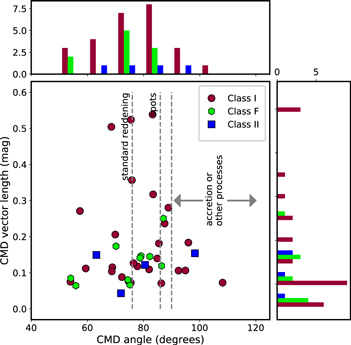
Figure 13. Distribution of CMD slope angles and length of the spanned vector in the CMD for the standard set of members. The majority of the sources show CMD angles compatible with extinction and spot modulation.
Download figure:
Standard image High-resolution image
Of the five sources with angles >90°, four of them are class I. We discount SSTYSV J183005.52−020108.0 since the fit is within 1σ of vertical, leaving four true "bluing" sources. SSTYSV J183005.23−020206.5 and SSTYSV J182959.47−020106.4 are both class I; both have  mag. Both are also periodic sources, but the color changes are not phased. SSTYSV J183002.95−020342.2 is a class II source with a larger Δ 3.6 (= 0.18 mag). Here the color change is clearly a long-term trend, starting blue and getting steadily more red as time progresses, with a total change of about [3.6]–[4.5] = 0.15 mag; this is the largest observed among the "bluers." Finally, the class I SSTYSV J182957.07−015946.0 shows the most extreme angle, >108°. However, there are <20 days of color data on this source, since it is near the top of the two-color field.
As discussed in several other papers in this series (e.g., Poppenhaeger et al. 2015; Wolk et al. 2015), some light curves show CMD slopes that turn bluer when the star becomes fainter. Several explanations are possible, such as scattered light or perhaps unresolved binaries with brightness changes of one of the components. While bluing is consistent with some models of accretion, in the one case where ultraviolet and Hα data are available (the multiwavelength study of NGC 2264; Cody et al. 2014; Stauffer et al. 2015), bluing was not seen during the accretion outbursts. Previously, we found that sources with bluing slopes show variability on significantly longer timescales than sources compatible with variability by extinction or spot modulation. Here the sample is very small. However, three of the sources indicate a coherence time in excess of 3 days in at least one channel. The two periodic bluers have periods of 8.7 and 12.7 days; this is consistent with those previous findings that bluers tend to change slowly.
4.5. Correlation between X-Rays and IR Variability
As we have done previously in the study of GGD 12–15, we examined whether the variability metrics were different for X-ray-detected sources. This could happen if, for example, X-ray flares give rise to flux increases or color changes in the IR. This field was observed with the Chandra X-ray Observatory, 2010 June 20, about a year before the Spitzer observations discussed here. Overall, there do not appear to be any correlations between the X-ray variability observed during the X-ray observation in 2010 and the Stetson index as measured across the 38 days of monitoring in 2011. Class III, class II, and class I objects range from no to moderate X-ray variability. This is discussed in more detail by E. Winston et al. (2017, in preparation).
In Wolk et al. (2015), we found timescales (as quantified by coherence time) were shorter for stars that emitted X-rays, among the class II sources in GGD 12–15. In that case, the Anderson–Darling obtained 99% confidence that coherence timescales were different for the X-ray- versus non-X-ray-selected samples of class II objects. The X-ray sources had longer overall coherence timescales by a factor of about 2. We identified a brightness selection effect since X-ray sources tended to be drawn from only the brightest sources in the IR sample. This was accounted for by limiting both groups to class II objects brighter than [3.6] = 12. The effect persisted: even among this restricted sample, X-ray sources still had shorter coherence times.
In Serpens South, we cannot perform the exact analogous measurement. While there are 17 sources with class II SEDs, only three are X-ray sources. However, as discussed previously, the highly embedded nature of Serpens South tends to steepen the SED slopes of embedded stars. The net result is many classical T Tauri stars are measured to have flat SEDs.
We can use the more detailed class information derived using colors and Herschel extinction data from E. Winston et al. (2017, in preparation). Winston et al. find 36 class 2 sources within the YSOVAR fields; 12 of these are also X-ray sources. When we compare the 12 X-ray-detected class II sources identified by E. Winston et al. (2017, in preparation) with non-X-ray-detected but bright at [3.6] class II sources, we recover the trend identifying the coherence time as being shorter (in both [3.6] and [4.5]) at >3σ significance for bright X-ray class II sources. However, this is not a robust result. This is one correlation determined among almost 20 tested cases. Such tests need to be subjected to a correction for the number of "blind" correlation tests (Dunn 1959). Once this correction is applied, the result no longer stands at 99% confidence. However, the coincidence that shorter coherence times were noted for X-ray-bearing class II sources seen here and in GGD 12–15 is intriguing.
4.6. Serpens South in the YSOVAR Context
The YSOVAR project obtained synoptic IRAC data for 11 star-forming clusters, Serpens South being the least evolved of these clusters. There is also a related project focused solely on NGC 2264 that employs simultaneous optical and IR data (Cody et al. 2014; Stauffer et al. 2014, 2015). The current goal of the YSOVAR project is to perform and present a detailed analysis of each cluster. Once each individual cluster has been understood in its own context, there will be a focus on the ensemble properties. This is the purpose of the standard set of cluster members. As of this writing, however, over 700 YSOs in the standard set of cluster members have had their light curves analyzed. So it is already worthwhile to see how Serpens South compares with the seven other clusters for which detailed studies have been completed.
Completed mid-IR variability studies exist for seven other clusters: IC 1396A (Morales-Calderón et al. 2009), NGC 2264 (Cody et al. 2014; Stauffer et al. 2014, 2015), Lynds 1688 (Günther et al. 2014), IRAS 20050+2720 (Poppenhaeger et al. 2015), NGC 1333 (Rebull et al. 2015), GGD 12–15 (Wolk et al. 2015), and Mon R2 (L. A. Hillenbrand et al. 2018, in preparation). There is also a preliminary overview of all clusters (Paper I) and a cursory report on a few sources in Orion (Morales-Calderón et al. 2011). All analyses find very high levels of variability for YSOs.
In this section, we will focus on comparing the results from the five clusters that have been analyzed in a manner similar to Serpens South. The other very young clusters among the previous investigations are IRAS 20050+2720 and L1688; after Serpens South, these clusters have the next highest fraction of class Is and the highest class I:II ratio. In IRAS 20050+2720 (Poppenhaeger et al. 2015), about 70% of all YSOs were found to be variable despite a large number of sources having to be excluded due to pull-downs and other issues that prevented high-fidelity photometry. Serpens South shares both the variability fraction and the pull-down issue with IRAS 20050+2720.
To make comparisons among clusters as fair as possible, we focus only on the sources with at least five observations in each band so that a Stetson index can be calculated (Table 7). A similar analysis was carried out by Rebull et al. (2015; see their Table 5). In Serpens South, the most variable objects are the class I sources; about 80% are found to vary. Among the five other clusters, the biggest difference is found in IRAS 20050+2720, where only 68% of class I were found to be variable. Some of this might be due to luminosity issues. When the class I sample was limited to bright sources, 71% of the IRAS 20050+2720 class I sources were found to be variable. On the other hand, about 80% of the flat spectrum and class II sources in IRAS 20050+2720 are found to be variable, consistent with what is seen in Serpens South.
Table 7. Variable Fractions across Published YSOVAR Clusters (Two-color Sample)
| Subset | NGC 1333a | GGD 12–15a | L1688a | IRASa | Mon R2a | Serpens | Sum |
|---|---|---|---|---|---|---|---|
| 20050+2720 | South | ||||||
| Standard members | 130 | 141 | 54 | 156 | 174 | 85 | 740 |
| Variable std. members | 67 | 106 | 40 | 106 | 100 | 58 | 483 |
| Variable %b | 52 ± 4 | 75 ± 4 | 74 ± 6 | 68 ± 4 | 57 ± 4 | 68 ± 5 | 65 ± 2 |
| Periodic (std.) | 19 | 38 | 10 | 28 | ⋯ | 18 | 113 |
| Periodic % | 15 ± 4 | 27 ± 4 | 18 ± 5 | 18 ± 3 | ⋯ | 21 ± 5 | 20 ± 2 |
| Two-band light curves only | |||||||
| Standard members | 98 | 122 | 37 | 109 | 89 | 53 | 508 |
| Variable std. members | 51 | 93 | 26 | 76 | 66 | 39 | 351 |
| Variable % | 52 ± 5 | 76 ± 4 | 70 ± 8 | 70 ± 4 | 74 ± 5 | 74 ± 6 | 69 ± 2 |
| Total class I | 13 | 18 | 11 | 34 | 20 | 31 | 127 |
| Total class F | 19 | 20 | 13 | 27 | 22 | 12 | 113 |
| Total class II | 46 | 57 | 10 | 38 | 35 | 7 | 193 |
| Total class III | 20 | 27 | 3 | 10 | 12 | 3 | 75 |
| Stetson variables only | |||||||
| Variable class I | 10 | 17 | 10 | 23 | 18 | 25 | 103 |
| Variable class F | 14 | 19 | 10 | 23 | 16 | 9 | 91 |
| Variable class II | 27 | 45 | 6 | 29 | 28 | 5 | 140 |
| Variable class III | 0 | 12 | 0 | 1 | 4 | 0 | 17 |
| Variability % | |||||||
| Class I | 77 ± 9 | 94 ± 5 | 91 ± 6 | 68 ± 7 | 90 ± 6 | 80 ± 7 | 81 ± 4 |
| Class F | 74 ± 9 | 95 ± 5 | 77 ± 9 | 85 ± 6 | 72 ± 10 | 75 ± 15 | 81 ± 3 |
| Class II | 59 ± 8 | 79 ± 5 | 60 ± 14 | 76 ± 9 | 80 ± 6 | 71 ± 14 | 73 ± 3 |
| Total for disked stars | 65 ± 12 | 85 ± 13 | 76 ± 20 | 76 ± 12 | 81 ± 14 | 74 ± 12 | 77 ± 4 |
| Class III | 0 + 4 | 44 ± 10 | 0 + 25 | 10 ± 10 | 33 ± 13 | 0 + 25 | 23 ± 5 |
Notes.
aColumns 2–6 are adapted from Rebull et al. (2015) Table 4. bAll errors are established using a ∼68% binomial confidence interval (Wilson 1927) with some rounding to make them symmetric.Download table as: ASCIITypeset image
Since Serpens South is so young, it might be expected to be accretion dominated. Wolk et al. (2013, 2015) speculated that sources noted observationally to be bluing are doing so by accretion. If true, we would expect a high fraction of bluing sources here. Instead, sources that are clearly bluer continue to be rare; only four were found in Serpens South. This is a little under 8% of the cluster standard set. This is consistent with the 11%–16% such sources seen in GGD 12–15, L1688, and IRAS 20050–2720.
In addition to being the youngest, Serpens South is one of the smallest clusters, with about 50 standard members in the two-color region and about 85 overall. Nonetheless, the variability fractions observed are almost exactly those of the six clusters when averaged. The extreme youth of the cluster probably leads to the limited sample of class III sources, none of which are variable, although the sample is so small that no meaningful conclusion can be drawn from this. NGC 1333 remains an outlier with low variability in all classes, despite its comparable age and size.
5. Summary
We have presented an analysis of mid-infrared light curves of over 1500 stars in the Serpens South region. Of these, 85 are young stars fulfilling our definitions of the standard set of cluster members. We augment these 85 with eight more probable cluster members. Our main findings are as follows:
- 1.The variability fraction of sources with disks is high with 77% ± 13%, 74% ± 20%, and 59% ± 19% for SED classes I, flat, and II, respectively. We find very similar results for the color-based class assignment, with the exception of class 2, which is about 78% consistent with the other disked classes. This may indicate some contamination among the SED selected class IIs in the highly embedded cluster. Confining our results to the central region with two-color data, the variability rates are higher: 80% ± 7%, 75% ± 15%, and 71% ± 14% for SED classes I, F, and II, respectively. This is in almost exact agreement with the averages of the other YSOVAR clusters. Most of the variable cluster members (∼80%) are not periodic. The detected amplitudes of variability are typically in the range of 0.13 mag for disk-bearing sources, with some sources displaying amplitudes of over 0.5 mag in [3.6] and [4.5]. The class III sources are not detected to be significantly variable, consistent with the interpretation that photospheric cool spots are the main driver of variability for these stars.
- 2.Class I sources show both the highest fraction of variables and the largest brightness variations. Flat spectrum sources show the second highest variability fraction, but the variability rates and amplitude of the changes observed are statistically indistinguishable for all three classes of disk-bearing YSOs. It is not until class III that there is a significant dropoff on variability. The results in L1688, GGD 12–15, and IRAS 20050+2720 are almost identical.
- 3.Less than 3% of the stars not identified with the cluster appear variable. About one-third of these are short-period objects, probably rapidly rotating binaries. But many of the others show changes similar to the cluster members and may represent a lower mass or more embedded or fainter population than the ∼90 that were the focus of the analysis presented here.
- 4.The timescales for variability tend to be longer for more embedded sources. For class I sources, we find variability timescales reach beyond the limit of our data set. For the disk-free sources, we find a strong clustering around a coherence time of 1 day, which implies full timescales of 3–5 days.
- 5.Four sources out of 39 standard-set variables with well-measured slopes in the CMD get significantly bluer as they dim. All four are disk-bearing YSOs. This is similar to the fraction found for GGD 12–15, L1688, and IRAS 20050+2720. In near-IR colors (e.g., K versus H−K), the fraction of bluers approaches one-third (Rice et al. 2015). Following Wolk et al. (2013), this is suggestive of an accretion event, but many scenarios are possible.
- 6.We tested for different mid-IR variability properties among the cluster members that have been detected in X-rays. This experiment was of limited fidelity because the X-ray and IR samples were not observed contemporaneously. We find the variability fraction is indistinguishable between the X-ray-detected and other members, after controlling for different mid-IR brightness distributions of the sample. We find a weak trend that X-ray-detected class II objects change more slowly (i.e., on longer timescales) than class II objects not detected in X-rays. Among the X-ray-detected members, we find their X-ray flux count rate and amplitude of mid-IR variability are anticorrelated. This may be an effect of disk inclination, causing X-ray absorption by gas in the YSO–disk system. The sources that are the most variable in the mid-IR may be the ones we are observing more edge-on.
All light curves will be made available through the IRSA database. The Python-based analysis code (pYSOVAR) used for the analysis of the light curves and CMDs is available through https://github.com/YSOVAR.
This work is based on observations made with the Spitzer Space Telescope, which is operated by the Jet Propulsion Laboratory, California Institute of Technology, under a contract with NASA. Support for this work was provided by NASA through an award issued by JPL/Caltech. This publication makes use of data products from the Two Micron All Sky Survey, which is a joint project of the University of Massachusetts and the Infrared Processing and Analysis Center, California Institute of Technology, funded by the National Aeronautics and Space Administration and the National Science Foundation. This research made use of Astropy, a community-developed core Python package for Astronomy (Astropy Collaboration et al. 2013). This research has made use of the SIMBAD database and the VizieR catalog access tool (Ochsenbein et al. 2000), both operated at CDS, Strasbourg, France, and of data products from the Two Micron All Sky Survey, which is a joint project of the University of Massachusetts and the Infrared Processing and Analysis Center, California Institute of Technology, funded by the National Aeronautics and Space Administration and the National Science Foundation. H.M.G. acknowledges Spitzer grant 1490851. K.P. was funded through the Sagan Fellowship program executed by the NASA Exoplanet Science Institute. H.Y.A.M. and P.P. acknowledge support by the IPAC Visiting Graduate Fellowship program at Caltech/IPAC. P.P. also acknowledges the JPL Research and Technology Development and Exoplanet Exploration programs. R.A.G. gratefully acknowledges funding support from NASA ADAP grants NNX11AD14G and NNX13AF08G and Caltech/JPL awards 1373081, 1424329, and 1440160 in support of Spitzer Space Telescope observing programs. S.J.W. was supported by NASA contract NAS8-03060 (Chandra X-ray Center).
Facilities: Spitzer - Spitzer Space Telescope satellite, Chandra - .
Footnotes
- 12
We include SSTYSV J183002.98−020221.1, which is just over 1'' from CXOJ 18:30:03.03-020220.8 but exceeds the slightly different match distance used by E. Winston et al. (2017, in preparation).
- 13
We use Arabic numerals to denote the classes determined by this method. As such, we do not interpret these class 0 objects as protostars lacking a core, but instead as extremely embedded objects.
- 14
A more common definition is to use the position of the first local maximum in the ACF, but due to the low number of data points in our light curves, the noise in the ACF is large and this value is often not well defined.
- 15
In this paper, errors are established using a ∼68% binomial confidence interval (Wilson 1927). The asymmetry in the confidence interval is averaged out for simplicity.