


ABSTRACT
The pulse profile of PSR B1133+16 is usually regarded as a conal double structure. However, its multi-frequency profiles cannot simply be fitted with two Gaussian functions, and a third component is always needed to fit the bridge region (between two peaks). This would introduce additional, redundant parameters. In this paper, through a comparison of five fitting functions (Gaussian, von Mises, hyperbolic secant, square hyperbolic secant, and Lorentz), it is found that the square hyperbolic secant function can best reproduce the profile, yielding an improved fit. Moreover, a symmetric 2D radiation beam function, instead of a simple 1D Gaussian function, is used to fit the profile. Each profile with either well-resolved or not-so-well-resolved peaks could be fitted adequately using this beam function, and the bridge emission between the two peaks does not need to be a new component. Adopting inclination and impact angles based on polarization measurements, the opening angle ( ) of the radiation beam in a certain frequency band is derived from beam-function fitting. The corresponding radiation altitudes are then calculated. Based on multi-frequency profiles, we also computed the Lorentz factors of the particles and their dispersion at those locations in both the curvature-radiation and inverse-Compton-scattering models. We found that the Lorentz factors of the particles decrease rapidly as the radiation altitude increases. Besides, the radiation prefers to be generated in an annular region rather than the core region, and this needs further validation.
Export citation and abstract BibTeX RIS
1. INTRODUCTION
PSR B1133+16 is one of the nearest pulsars, located at a distance of  (Brisken et al. 2002). It has a period of
  (Hobbs et al. 2004) and is characterized by a dispersion measure of
  (Hassall et al. 2012). Its pulse profiles have previously been analyzed to map the radius–frequency relations (Cordes 1978; Thorsett 1991; Xilouris et al. 1996; Mitra & Rankin 2002). Because of the long period and small dispersion measure of PSR B1133+16, the impact on its profile of the effects of both dispersion and scattering is small. This renders its profile highly suitable for analysis of the radio radiation beam. The profiles of PSR B1133+16 are usually treated as "well-resolved conal-double" profiles (Rankin 1983), and it is therefore natural to fit the profiles with a two-component model. However, the integrated profiles cannot be fitted satisfactorily in the bridge region between the peaks, and hence an additional component had to be added to optimize the fit results (Hassall et al. 2012). In fact, an obvious bulge appears in simulated low-frequency profiles when using three components to simulate the profiles (Hassall et al. 2012), but this is not present in real profiles (Phillips & Wolszczan 1992; Karuppusamy et al. 2011). Based on the derived best-fitting parameters, the different radiation models and the location of the radiation could be verified and validated.
The radiation mechanism of pulsar radio emission is still not well understood. Nevertheless, a variety of models have been proposed, and certain pulse profiles are predicted by different models. In the curvature-radiation (CR) model, the radiation beam is always regarded as a single conal component. Consequently, the pulse profile should be composed of either a single peak or double peaks (Ruderman & Sutherland 1975; Wang et al. 2013). The nature of the core emission in the CR model has also been discussed (Gil & Snakowski 1990; Beskin & Philippov 2012). It could explain some pulsars' pulse profiles. On the other hand, the inverse-Compton-scattering (ICS) model includes one core and two conal components, and thus the number of pulse peaks could range between one and five (Qiao & Lin 1998; Qiao et al. 2001). This could be consistent with the observational evidence (Rankin 1983; Hankins & Rickett 1986). Based on observations of the pulse profiles, a beam composed of one core and two conal components could be plausible (Rankin 1983), but the radio radiation mechanism of pulsars has not yet been determined unequivocally. The radio radiation location of pulsars is yet another puzzle. Even if just the so-called inner-gap model is considered, one needs to distinguish between the core gap model (Ruderman & Sutherland 1975) and the annular gap model (Qiao et al. 2004a).
In this paper, a conal double model is used to fit the PSR B1133+16 profiles at several frequencies. In Section 2, the observation and our data reduction approach are introduced. The pulse profiles are fitted using the conal double model in Section 3. The energy of particles in the magnetosphere is analyzed by considering the radiation mechanism, as discussed in Section 4. Some remaining issues are discussed in Section 5, and our conclusions are presented in Section 6.
2. OBSERVATION AND DATA REDUCTION
Observations at a central frequency of 2256 MHz were made with the Kunming 40 m Telescope of Yunnan Astronomical Observatory, Chinese Academy of Sciences (CAS). This telescope is located in Yunnan Province, China, at longitude 102 8 E and latitude +250 N (Hao et al. 2010). The signal was folded using the Pulsar Digital Filter Bank 3 with parameters provided by PSRCAT9
(version 1.51). The observations are affected by radio-frequency interference (RFI) due to the wireless-fidelity (Wi-Fi) network. This noise was removed manually with the software package PSRCHIVE.10
Observations at a central frequency of 8600 MHz were obtained with the Tianma 65 m Telescope, located at longitude 1211 E and latitude +309 N. The telescope is located at the Shanghai Astronomical Observatory, CAS. The 8600 MHz signal was folded using the Digital Backend System. The relevant observational information is included in Table 1. The raw data at these two frequencies were added to profiles with PSRCHIVE. The 317 MHz data were obtained with the Giant Metrewave Radio Telescope (GMRT).
8 E and latitude +250 N (Hao et al. 2010). The signal was folded using the Pulsar Digital Filter Bank 3 with parameters provided by PSRCAT9
(version 1.51). The observations are affected by radio-frequency interference (RFI) due to the wireless-fidelity (Wi-Fi) network. This noise was removed manually with the software package PSRCHIVE.10
Observations at a central frequency of 8600 MHz were obtained with the Tianma 65 m Telescope, located at longitude 1211 E and latitude +309 N. The telescope is located at the Shanghai Astronomical Observatory, CAS. The 8600 MHz signal was folded using the Digital Backend System. The relevant observational information is included in Table 1. The raw data at these two frequencies were added to profiles with PSRCHIVE. The 317 MHz data were obtained with the Giant Metrewave Radio Telescope (GMRT).
Table 1. Observational Information
| 2256 MHz Data | |
|---|---|
| Telescope | Kunming 40 m radio telescope |
| Number of pulse phase bins | 512 |
| Center frequency (MHz) | 2256 |
| Bandwidth (MHz) | 251.5 |
| System temperature (K) | 80 (Hao et al. 2010) |
| SEFDa (Jy) | 350 (Hao et al. 2010) |
| Observation duration (s) | 38983 |
| Start UT | 07:17:02 |
| Start MJD | 56802 |
| Start second | 26240 |
| 8600 MHz Data | |
| Telescope | Tianma 65 m radio telescope |
| Number of pulse phase bins | 1024 |
| Center frequency (MHz) | 8600 |
| Bandwidth (MHz) | 800 |
| System temperature (K) | 35 |
| SEFD (Jy) | 50 (Yan et al. 2015) |
| Observation duration (s) | 5354 |
| Start UT | 11:44:49 |
| Start MJD | 56836 |
| Start second | 42288 |
Note.
aSystem equivalent flux density.Download table as: ASCIITypeset image
Apart from the 317, 2256, and 8600 MHz data, other observations with central frequencies of 116.75, 130, 139.75, 142.25, 147.5, 156, 173.75 MHz (Karuppusamy et al. 2011), 408, 610, 925, 1642 MHz (Gould & Lyne 1998), 1410, 1710, and 4850 MHz (von Hoensbroech & Xilouris 1997) have also been adopted here. The data for the final seven frequencies were downloaded from the European Pulsar Network (EPN) Data Archive.11
The multi-frequency profile of PSR B1133+16 is shown in Figure 1. All profiles have been normalized by their maximum flux densities and are aligned at phase  , which was obtained by fitting the profile to Equation (6). The profile of PSR B1133+16 is well resolved, exhibiting a conal double structure.

Figure 1. Multi-frequency profile of PSR B1133+16. All profiles have been normalized by their maximum flux densities and are aligned at phase  , which was obtained by fitting the profile to Equation (6).
Download figure:
Standard image High-resolution image3. PULSE PROFILE COMPONENT ANALYSIS OF PSR B1133+16
3.1. Numerical Experiment Assessing the Profiles of a Single Conal Component
First, we will perform a numerical experiment pertaining to our component analysis. The intensity of a radiation beam composed of a single conal component is related only to the angle between the radiation direction and the magnetic axis (henceforth referred to as  ), and its radiation exists if and only if
  attains a value in a specific narrow range. A Gaussian intensity distribution,
  , is assumed in the experiment,

where

The model's 3D waterfall graph is shown in Figure 2. The parameters A, r0, and σ are set to 1.0, 1.2, and 0.2, respectively. The section planes of the conal component for different y values are similar to sections traversed by the radiation beam's line of sight for different impact angles. The section profiles can be regarded as pulse profiles. From the section profiles, two peak components and a bridge component between the two peaks can clearly be seen. Upon trying to fit these profiles with both a two-peak model (see Figure 3) and a three-peak model (see Figure 4), one can see significant residuals and inconsistencies in the bridge region for the two-component profile fit. (The Levenberg–Marquardt algorithm was used to fit the profiles, and is also adopted below.) On the other hand, the three-peak model leaves small residuals, but the width of the central peak is too large to treat it as an independent component. This characteristic may be an efficient tool to distinguish the bridge component.
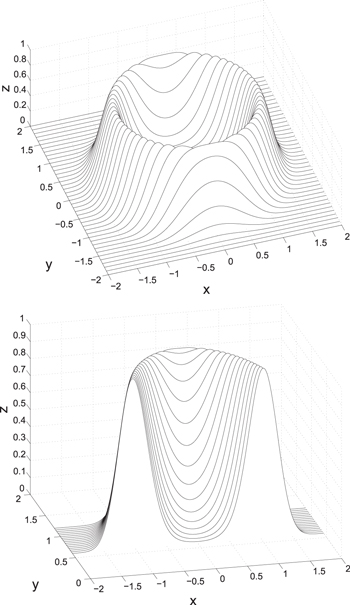
Figure 2. Top: radiation conal component; bottom: cut-out section. The height shows the intensity of the radiation beam. The curves show sections along the line of sight, i.e., pulse profiles. The bridge component is clearly seen.
Download figure:
Standard image High-resolution image
Figure 3. Fits based on two Gaussian components of the sections in Figure 2 for different y values. The thin lines (blue) are the sections. The dashed lines (green) represent the two peaks, and the thick lines (red) trace the combination of the two peaks. The blue dashed lines show the fit residuals, adopting the same units as in the main panels.
Download figure:
Standard image High-resolution image
Figure 4. As Figure 3, but for fits with three Gaussian components.
Download figure:
Standard image High-resolution image3.2. Determining the Shape of the Conal Component
In the multi-component analysis of the pulse profile, a Gaussian function with  wing dampening is usually used as the peak function (Kramer 1994; Wu et al. 1998). However, the shape of the conal component in the real pulse profile is as yet unknown. In this paper, to determine the most probable shape of the conal component, the following four functions are also used as trial peak functions to fit the pulse profile:


In Equation (2), the factor has been chosen to make the function resemble a Gaussian function, while in Equations (3)–(5), the factors have been chosen such that all functions have the same height, central position, and area as the equivalent Gaussian function, since the same parameters are used. The von Mises function (Equation (2)) has also been used to fit the pulse profile (Manchester et al. 2013), since it has a similar shape to the Gaussian function and is periodic. The hyperbolic secant function (Equation (3)) and the square hyperbolic secant function (Equation (4)) naturally have exponential wings. These two functions also show a peaked distribution; they have larger kurtosis and higher wings than the Gaussian function. The Lorentz function is characterized by inverse-square decreasing wings. The curves of Equations (3)–(5) and the Gaussian function are shown in Figure 5. Since the von Mises function has a similar curve to the Gaussian function, it has not been plotted. As shown in Figure 5, the Gaussian function has steeper wings than the square hyperbolic, the hyperbolic, and the Lorentz functions.
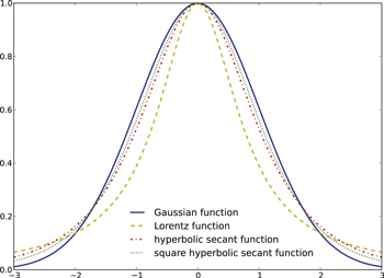
Figure 5. Gaussian, Lorentz, hyperbolic secant, and square hyperbolic secant functions. In all cases, the location, height, and width are all set to 1.
Download figure:
Standard image High-resolution imageAs shown in Figure 6, these five functions have been used to fit the 2256 MHz pulse profile of PSR B1133+16. Ignoring the trailing wings, which may be affected by interstellar scattering, we have thus shown that exponential damping functions such as the hyperbolic secant or square hyperbolic functions provide better fits to the leading wings. The leading-wing residuals of the multi-frequency profiles are shown in Table 2. By comparing the root-mean-squares of the leading-wing residuals, the fit based on the square hyperbolic secant function has the smallest leading-wing residuals in most cases, and it also has the smallest maximum and average residuals. Using the minimax criterion and Akaike's information criterion (AIC), which is defined as  , where k is the number of parameters and
  is proportional to
  (Burnham & Anderson 2002), the square hyperbolic secant function is adopted as the most appropriate shape of the conal component to fit the pulse profile. Because the square hyperbolic secant function is judged to be the best peak function to fit the profiles, the PSR B1133+16 profiles are fitted with three square hyperbolic secant peaks. This fit yields a very wide central peak, similar to that found experimentally (see Figure 7; only the eight frequency profiles that include a bridge component have been taken into account in the fits), and it thus implies that the bridge component of the PSR B1133+16 pulse profile cannot be independent.

Figure 6. Fits of the observed 2256 MHz profile of PSR B1133+16 with five different functions. The profiles have been aligned with the highest point of the first peak, and the pulse phase at the corresponding point is defined as  . The five panels separately show fits with a Gaussian function (left-hand panel, first row), a von Mises function (right-hand panel, first row), a hyperbolic secant function (left-hand panel, second row), a square hyperbolic secant function (right-hand panel, second row), and a Lorentz function (bottom panel). σ: root-mean-square of the residuals of the leading wings (for points with a pulse phase
  ). The square hyperbolic secant function yields the best-fitting results in the leading-wing region, with the smallest σ.
Download figure:
Standard image High-resolution image
Figure 7. Three-peak fits of the PSR B1133+16 multi-frequency profile. Only the profiles that include a bridge component have been taken into account in the fits. The green dashed lines highlight the three peaks, while the thick red line represents the combination of the three peaks. The thin blue lines are the observed profiles. The width of the central peak is too large to treat it as an independent component.
Download figure:
Standard image High-resolution imageTable 2. Leading-wing Residuals of the Fits with Five Test Functions
| Freq. (MHz) | G | M | H | S | L |
|---|---|---|---|---|---|
| 317 | 0.0146 | 0.0146 | 0.0128 | 0.0096 | 0.0483 |
| 408 | 0.0053 | 0.0053 | 0.0175 | 0.0064 | 0.0571 |
| 610 | 0.0047 | 0.0047 | 0.0186 | 0.0063 | 0.0596 |
| 925 | 0.0097 | 0.0097 | 0.0177 | 0.0083 | 0.0568 |
| 1410 | 0.0121 | 0.0121 | 0.0081 | 0.0098 | 0.0341 |
| 1642 | 0.0096 | 0.0096 | 0.0167 | 0.0064 | 0.0518 |
| 1710 | 0.0099 | 0.0099 | 0.0085 | 0.0081 | 0.0299 |
| 2256 | 0.0176 | 0.0176 | 0.0083 | 0.0072 | 0.0367 |
| Maximum | 0.0176 | 0.0176 | 0.0186 | 0.0098 | 0.0596 |
 (10−5) (10−5) |
12.6 | 12.6 | 20.2 | 6.2 | 230.7 |
Note. Columns marked G, M, H, S, and L represent the leading-wing residuals of the fits with Gaussian, von Mises, hyperbolic secant, square hyperbolic secant, and Lorentz functions, respectively, and  is the average value of the
  's of all eight frequencies.
Download table as: ASCIITypeset image
3.3. Profile Fits with a Conal Double Model
In modeling the actual radiation beam, asymmetries caused by pulsar rotation should be taken into account. This effect leads to differences in the radiation intensity of the conal component with pulse phase, ϕ. Here we consider only the first order (i.e., the linear variation) of the radiation intensity. In the conal double model, the conal component can be expressed as

Here,  can be obtained from ϕ (Zhang et al. 2007),

where α is the magnetic inclination angle and β the impact angle. In Equation (6), A is the amplitude of the Gaussian function,  and σ are the angular radius and angular width of the radiation conal component, k is the first order of the radiation intensity, which varies with ϕ and also represents the conal component's asymmetry, and
  is the phase measured when the line of sight, the magnetic axis, and the rotation axis are coplanar.
In the fit, we adopt inclination and impact angles of  and
and  , respectively (Lyne & Manchester 1988). The resulting pulse profile fit for PSR B1133+16 with this conal double model is shown in Figure 8. The bridge components could clearly be fitted adequately. The residuals in excess of the uncertainties in the data are caused by both our adoption of a square hyperbolic secant profile and our assumption of linear variation of the radiation intensity. Aberration and retardation may also affect the shape of the conal component (Kumar & Gangadhara 2013). The error due to model selection bias is much larger than the system noise, which shows that the system noise does not affect our analysis. The fit parameters as a function of frequency are included in Table 3 and shown in Figure 9. The uncertainties in the parameters were calculated based on application of the Jacobian matrix around the best-fitting solution. Since the amplitudes (A) and initial positions (
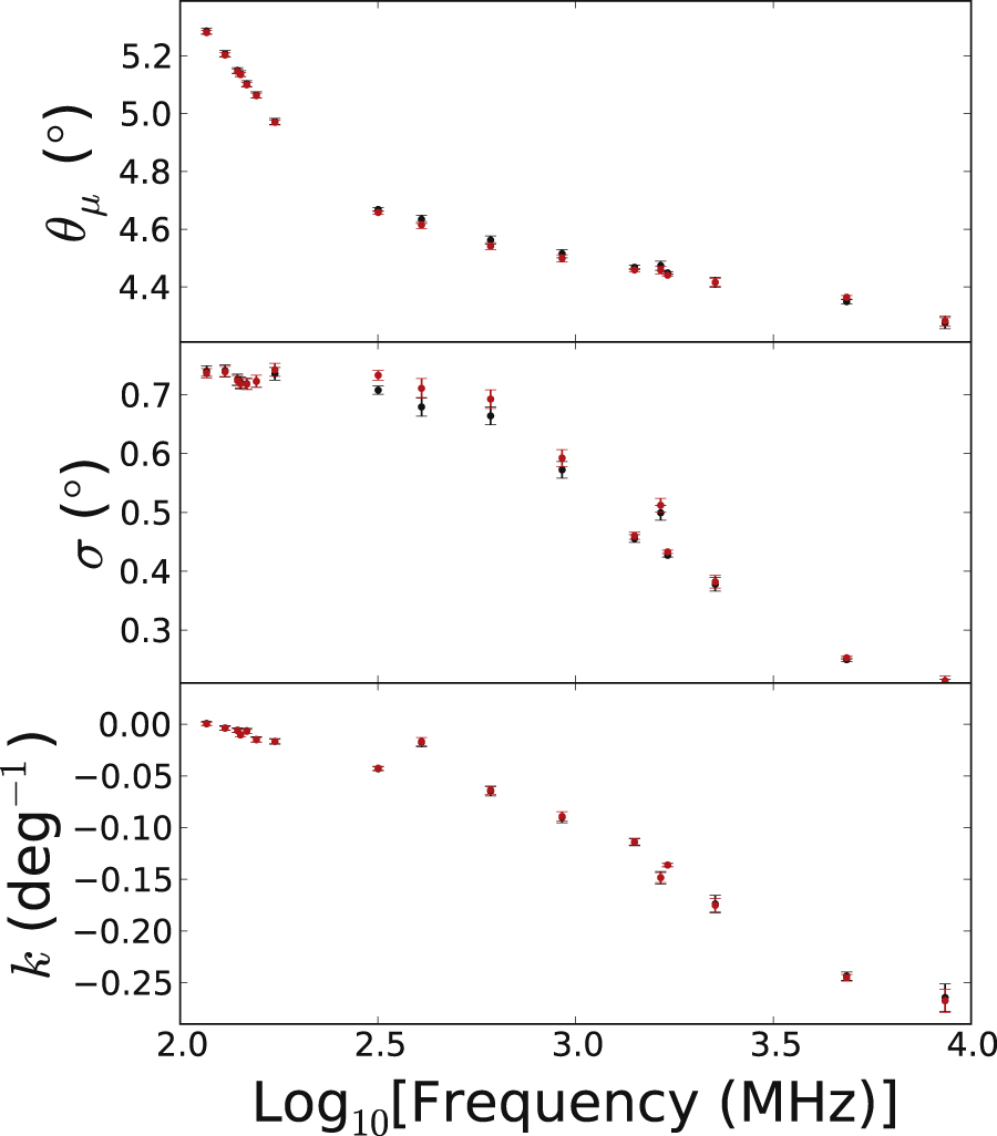
 ) of the profile are not important, we show only the other three parameters. In Figure 9, the parameters obtained by performing fits with a Gaussian-shaped conal component are also shown for comparison. They are approximately the same as for the fit obtained with a square hyperbolic secant profile. As shown in this figure, the opening angle of the radiation cone decreases with frequency, which means that the phase difference between the two peaks increases. This phenomenon occurs for most pulsars (Chen & Wang 2014). In the following, only the results calculated based on the square hyperbolic secant profile are adopted.

Figure 8. Conal double model fits of the PSR B1133+16 multi-frequency profiles. The blue dotted lines are the observed profiles, while the red solid lines are the best-fitting results.
Download figure:
Standard image High-resolution image
Figure 9. Best-fitting parameters of the conal double model vs. frequency. From top to bottom, the parameters are the conal radius ( ), the conal width (σ), and the conal asymmetry (k). The fit results of Equation (6) are plotted as red points with error bars, and the black markers are the results of fits with a Gaussian-shaped conal component.
Download figure:
Standard image High-resolution imageTable 3. Fit Parameters for the Conal Double Model
| Freq. (MHz) |
 (deg) (deg) |
σ (dcg) | k (deg−1) |
|---|---|---|---|
| 116.75 | 5.283 ± 0.008 | 0.737 ± 0.008 | 0.001 ± 0.002 |
| 130 | 5.205 ± 0.008 | 0.739 ± 0.009 | −0.004 ± 0.002 |
| 139.75 | 5.148 ± 0.008 | 0.724 ± 0.009 | −0.006 ± 0.002 |
| 142.25 | 5.137 ± 0.008 | 0.719 ± 0.009 | −0.010 ± 0.002 |
| 147.5 | 5.102 ± 0.008 | 0.718 ± 0.009 | −0.007 ± 0.002 |
| 156 | 5.064 ± 0.009 | 0.72 ± 0.01 | −0.015 ± 0.002 |
| 173.75 | 4.971 ± 0.009 | 0.74 ± 0.01 | −0.017 ± 0.002 |
| 317 | 4.662 ± 0.006 | 0.723 ± 0.008 | −0.043 ± 0.002 |
| 408 | 4.62 ± 0.01 | 0.70 ± 0.02 | −0.017 ± 0.004 |
| 610 | 4.55 ± 0.01 | 0.68 ± 0.02 | −0.064 ± 0.004 |
| 925 | 4.51 ± 0.01 | 0.58 ± 0.01 | −0.090 ± 0.005 |
| 1410 | 4.463 ± 0.007 | 0.459 ± 0.006 | −0.114 ± 0.003 |
| 1642 | 4.47 ± 0.01 | 0.51 ± 0.01 | −0.148 ± 0.005 |
| 1710 | 4.444 ± 0.003 | 0.431 ± 0.003 | −0.136 ± 0.002 |
| 2256 | 4.42 ± 0.02 | 0.38 ± 0.01 | −0.174 ± 0.007 |
| 4850 | 4.358 ± 0.006 | 0.251 ± 0.003 | −0.245 ± 0.003 |
| 8600 | 4.28 ± 0.02 | 0.211 ± 0.008 | −0.27 ± 0.01 |
Download table as: ASCIITypeset image
4. RELATIVISTIC PARTICLES IN THE MAGNETOSPHERE
4.1. Radiation Altitude
Before analyzing the distribution of the particle energies in the magnetosphere, the radiation altitude for each frequency band must be calculated. The radiation altitude can be calculated under the assumption of a dipole field and also assuming that the radiation is emitted near a specific field line, since the pulse phase ϕ is fixed. First, the equation describing the dipole field line can be written as

where r and θ are spherical coordinates with the magnetic axis in the zenith direction and  is the field line's diameter. The latter is a fixed parameter for a specified field line. This specified field line could be either in the core region or in an annular region (Qiao et al. 2004a, 2007). The field line in the core region is set at 0.75 times the critical field line (which passes the point of intersection between the null charge surface and the light cylinder) for the zenith angle of the point of intersection between the field line and the pulsar surface. The field line in the annular region is set at the average value of the critical field line and the last opening field line (which is tangential to the light cylinder, and which can be calculated following the method of Zhang et al. 2007). All of these field lines are shown in Figure 10. The dotted line shows the real shape of the radiation beam (the core region's field line is marked blue, while the annular region's field line is marked red). The last opening field line is shown as the black solid line and the critical field line is rendered as the black dashed line. In the top panel, a section of the field lines in the polar-cap region is shown, while a 2D sketch of the radiation beam is offered in the bottom panel. The detailed calculation of
  of the critical field line is given in Appendix
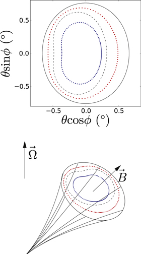
Figure 10. Field line in the core region (blue dotted line) and in the annular region (red dotted line). The black solid curve is the last opening field line, and the black dashed line is the critical field line. Top: section in the polar region; bottom: 2D radiation beam.
Download figure:
Standard image High-resolution imageCombined with the assumption that the radiation is emitted along the tangent line of the magnetic field, the relation between θ and  can be obtained:

With Equations (7) and (8), the radiation's position can be determined: see Figure 11. In the top panel, the radiation altitude for different radiation regions is shown, revealing that higher-frequency photons come from lower positions in the pulsar. In the bottom panel, the relative radiation altitudes for different radiation regions are plotted. It is apparent that the radiation position in the core region's model is significantly higher than that in the annular region's model.

Figure 11. Radiation altitude. The blue markers show the results for the core region, while the red markers show the results pertaining to the annular region. The plane defined by the rotation and magnetic axes is shown in the bottom panel. The black solid curve represents the last opening field line, while the black dashed line shows the critical field line.
Download figure:
Standard image High-resolution image4.2. Particle Energy Loss
In both the ICS and CR models, the energy of the radiating particles can be calculated if the radiation frequency and position are known. The radiation frequency in the CR model,  , can be calculated from the Lorentz factor of the particles, γ, and the curvature radius, ρ, of the field line (Ruderman & Sutherland 1975),

where c is the speed of light and

and this approximation applies to the case  . Based on Table 3 and Equation (8), θ could be still smaller than 4°, and the approximation above should be always valid. The particle energy can then be obtained in the CR model. In the ICS model, the radiation frequency,
  , can be expressed (Zhang et al. 2007) as

where  is the initial frequency of the photons generated by gap sparking, which is about 1 MHz before scattering,
  , and
, and


where  and
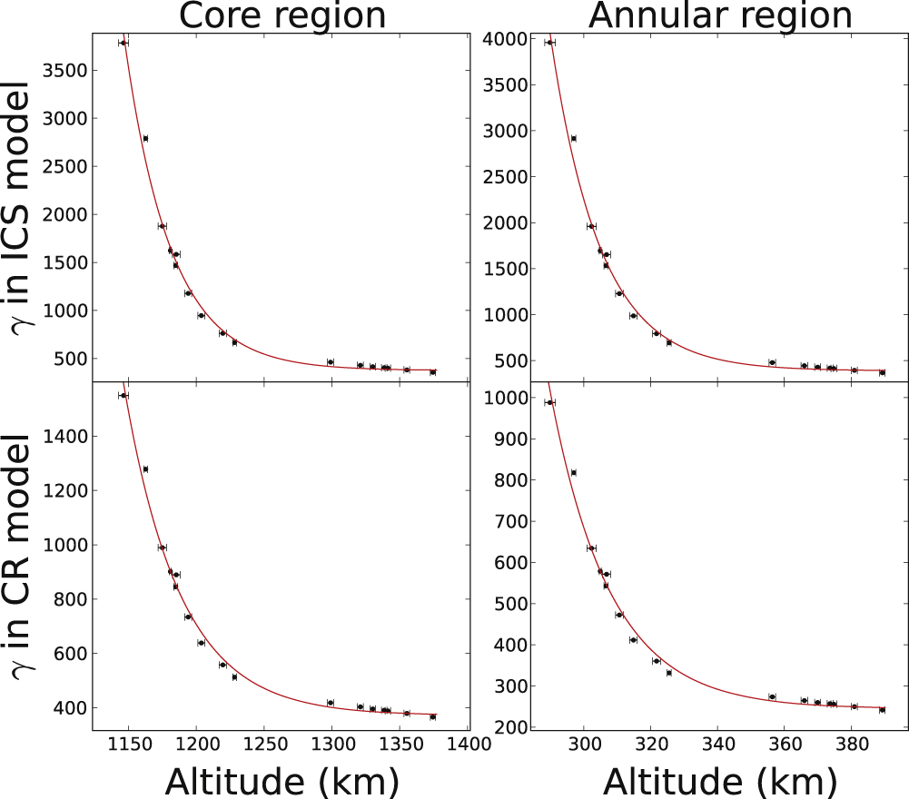
and  are the polar coordinates of the initial photon-radiation position and R is the radius of the pulsar. The particle energy can then also be obtained in the ICS model. The results are shown in Figure 12, which suggests that the particle energy should decrease with altitude in both the ICS and the CR models, i.e., the particles would lose energy while moving along the magnetic field lines. This result is consistent with the assumptions adopted in some previous studies regarding the ICS model (Qiao & Lin 1998; Qiao et al. 2001; Zhang et al. 2007).
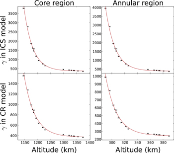
Figure 12. Evolution of particle energy with altitude for different cases. Fits to the data points using Equation (11) are also shown.
Download figure:
Standard image High-resolution imageAs shown in Figure 12, the rate of decrease of the particle energy also decreases with altitude. The functional form describing the particle energy as a function of altitude H is suggested to be exponential, as was also adopted in a number of previous studies (Zhang et al. 2007; Wang et al. 2013),

The points in Figure 12 are fitted with this function; the result is shown in Table 4 and it is also presented in the figure. Note that A is not the initial Lorentz factor of particles but just a fitting parameter, since the Lorentz factor of particles beyond the radiation region that generates emission with the frequencies chosen above is hard to estimate. From the figure, the Lorentz factors of the particles have a lower limit of ∼300. In other words, only high-energy particles would lose energy in the magnetosphere. This phenomenon cannot be explained by other, traditional models of the magnetosphere.
Table 4. Results of Fits to the Data Points in Figure 12 Using Equation (11)
| Case | γ1 | A | H0 (km) |
|---|---|---|---|
| Core (ICS) | 380 ± 70 | (1.18 ± 0.07) × 1018 | 34.28 ± 0.01 |
| Core (CR) | 370 ± 30 | (1.24 ± 0.07) × 1015 | 41.46 ± 0.02 |
| Annular (ICS) | 390 ± 80 | (1.01 ± 0.06) × 1012 | 14.92 ± 0.02 |
| Annular (CR) | 240 ± 20 | (7.8 ± 0.5) × 109 | 17.97 ± 0.03 |
Download table as: ASCIITypeset image
4.3. Particle Energy Dispersion
In the CR model, the conal beam width can be derived based on Equations (7)–(9) and the assumption  , i.e.,

where  is the full width at half maximum of the conal component,
  is the bandwidth of each band, and
  is the dispersion of γ. Note that
  is not the Lorentz factor dispersion of the particles at a certain location but the Lorentz factor dispersion of the particles that emit photons with the same phase. From Equation (12) it follows that, for a specified frequency, the conal width can be determined from the radiation field line and the particle energy dispersion. As the field line does not change with radiation frequency, any change in the conal width as the frequency increases is due to variation in the particle energy dispersion with altitude.
In the ICS model, the conal width can also be derived from Equation (10) and the assumptions  ,
,  , and
, and  ,
,

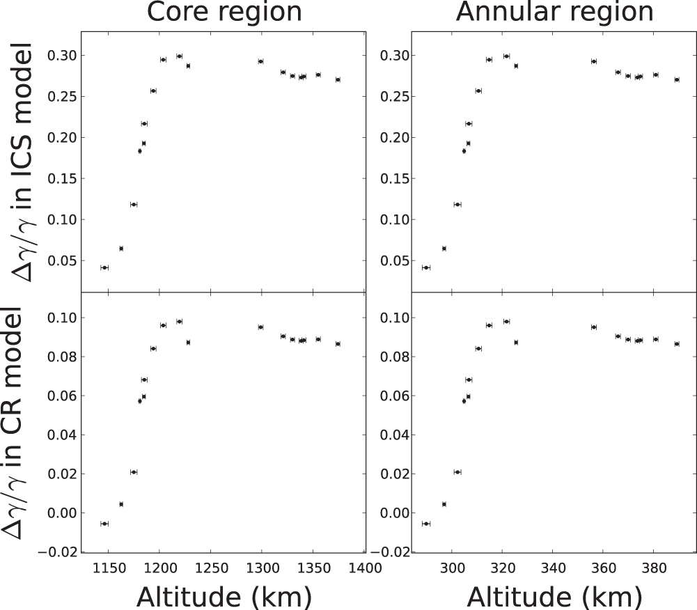
Similarly, the conal width changes as a result of the variation in particle energy dispersion. With Equations (12) and (13),  can be calculated. The results are shown in Figure 13. In this figure and below, the particle energy dispersion is expressed as
  .
.

Figure 13. Particle energy dispersion vs. altitude, represented by  . As shown in Figure 12 and here, the variation in particle energy is similar to that relating to the particle energy dispersion. The particle energy decreases rapidly while the particle energy dispersion increases sharply. On the other hand, as the rate of decrease becomes smaller, the dispersive process comes to a halt. These particle-energy properties provide constraints on the physical processes in the magnetosphere.
Download figure:
Standard image High-resolution imageIn fact, radiation emitted in the same phase of the profile also originates from different field lines. This means that  not only includes the width of the particle spectrum but also contains energy variations around the locations calculated in Section 4.1. In this case, the latitudinal distribution of the particles would also contribute to
  . Under the assumption of the presence of a core gap or an annular gap, the initial latitudinal distribution of particles and particle energy should be consistent. In other words, the latitudinal difference of particles in the vicinity of the radiation location is equivalent to the latitudinal energy dispersion.
As shown in Figure 13, the particle energy disperses as altitude increases in the lower region, but in higher regions it does not yet change. This change in energy dispersion is similar to that of the energy-loss process, which is analyzed in Section 4.2. This may imply that the decrease and dispersion in particle energy are caused by the same physical process. From Figure 13 it follows that, in the ICS model, the particle energy dispersion could still be positive, and the negative particle dispersion at lower altitudes cannot be explained if the CR model is adopted. The particle energy dispersion could be used to determine that there is a weak bridge component at both high and low frequencies. For low frequencies, the conal radius is located far above the impact angle, and measurements along the line of sight would produce two almost independent peaks. However, at high frequencies, the conal component is narrower because of the narrower particle energy spectrum, and the bridge component would also disappear. This is also the reason why only the profiles observed in mid-frequencies have obvious bridge components, and thus why eight profiles are chosen in Figure 7.
5. DISCUSSION
The pulse profile of PSR B1133+16 has two obvious peaks. Assuming that these two peaks are two independent components, the profile should be fitted by adopting a two-peak model. In fact, the bridge region between the two peaks cannot be adequately fitted in the two-peak model, which implies that the two peaks cannot be regarded as independent components. Three-peak model fits yield a central component that is too wide in the bridge region, which means that the bridge component could be an artificial one. On the other hand, an emission model with more than three components is too complex for this source and cannot be made to agree with core or conal emission geometries. In addition, the profile can be fitted very well with a 2D conal function, which has fewer parameters (five) than even the two-peak model (six parameters). It also implies that the two peaks should be the natural result of real conal components of radiation.
In Section 4, we demonstrated that radiation of different pulse phases is related to the particle energy at the radiation position and that the widths of peaks can be understood as the width of the particle energy spectrum, to some extent. If so, the flux of the wings versus the pulse phase could be naturally regarded as the manifestation of a particle energy spectrum. In the ICS and CR models, the Gaussian peak may imply that particles at the radiation position have an energy spectrum resembling  , but there is no reasonable physical process that could result in such a spectrum. Conversely, a power-law or exponential spectrum could be understood more easily. Peak functions with power-law or exponential wings, such as a Lorentz function, a hyperbolic secant function, or a square hyperbolic secant function, may be better physically motivated to fit the pulse profile, and fits using a square hyperbolic function indeed yield a better result. The angular distribution of the particles could also affect the damping rate of the wings, and whether the particle spectrum or its angular distribution plays a leading role in this aspect needs to be studied in more detail.
The notion that peak functions with exponential wings lead to better fit results, as mentioned in Section 3, also applies to other pulsar profiles. In other words, the pulse profile components may have a shape similar to the square hyperbolic secant function. This insight should be considered in pulsar timing. For example, while constructing a profile template, the square hyperbolic secant function could be used to fit the template profile instead of Gaussian or von Mises functions.
As shown in Figure 11, the range of radiation altitudes for different frequencies depends significantly on the assumption adopted for the radiation region. The difference in radiation altitude between 116.75 and 8600 MHz is 228 km for the core-region radiation assumption and only 100 km if we assume that the radiation originates in an annular region. As a consequence, a time lag of 0.76 ms is predicted between 116.75 and 8600 MHz for core-region radiation, but only 0.33 ms for annular-region radiation. Such effects would significantly affect simultaneous multi-frequency pulsar timing results if the same template is used for profiles at different frequencies in pulsar timing. In other words, timing may be an effective method to distinguish the location of the radiation region, but the dispersion measure (DM) should first be determined accurately.
The positive correlation between the absolute value of the conal asymmetry and the pulsar frequency is shown in Figure 9. It is apparent that the asymmetry varies continuously as the radiation localization increases in altitude. It leads to a smaller and smaller trailing peak (relative to the leading peak) as frequency increases, and in a very high frequency band the trailing peak could be predicted to be vanishing. Such asymmetry may be caused by the inhomogeneous distribution of the parallel electric field in the polar gap, which may be a result of pulsar rotation, and the density and spectrum of the particles would be different for different azimuth angles of the conal component. In addition, in the context of the ICS model, the conal asymmetry could also be due to the asymmetry of the initial photon energy distribution. If the luminosity of the initial photons in the polar-cap region is inhomogeneous, the radiation flux density would vary for different magnetic field lines. The inhomogeneity of the photon field weakens with increasing altitude, because the differences in the distance between the polar cap and different radiation locations become smaller. The asymmetry of the pulse profile would thus disappear. While this effect is reflected in the pulse profiles, the asymmetry would increase with increasing frequency, which is consistent with the observations.
Other effects, such as field-line bending caused by pulsar rotation, aberration, retardation, and plasma effects, could also affect the shape of the profile. The first three effects would affect the arrival time of the radiation, and the time difference  characteristic of all three effects can be estimated:
  , where
  is the altitude difference between the radiative locations in a given band. This altitude difference could also be estimated as
  . If the radiation is generated in the core region,
  , while for an annular region,
  . Given that the period of PSR B1133+16 is 1.1879 s, these three effects cannot significantly affect the observed profile. The uneven plasma distribution in the magnetosphere could lead to light deflection, which would result in deformation of the pulse profile. Using the laws of reflection, the deflection angle
  could be derived,
  , where
  is the electron plasma frequency and
  is the electron cyclotron frequency at the radiation location. Adopting the Goldreich–Julian density (Goldreich & Julian 1969) as the density of the free charged particles in a plasma, this deflection angle can be calculated. For the core, the deflection angle can be up to
  if the lowest frequency 116.75 MHz is adopted, while for the annular region, this value is
  . Even if the magnetic field is ignored, the deflection angle, which is expressed as
  , attains values of
  and
and  for the two cases. These results show that plasma effects are insignificant for our analysis of the profiles of PSR B1133+16. As discussed above, these effects would not change the distance between the two peaks or their widths significantly, so that they will not affect the results obtained in Section 4.
The initial frequency of the photons before scattering,  , is decided by both theories and observations. From theories in the RS model (Ruderman & Sutherland 1975), a low-frequency wave is produced in the inner gap sparking, which means the timescale should be
  . In the RS model, only the curvature radiation is taken into account, but near the star's surface the strong magnetic field effects should also be taken into account. When such effects are considered, the gaps should be nearly five times lower than RS's (Zhang et al. 1997). From observations, the occasional sub-pulses with a time structure shorter than
  (Hankins 1971; Bartel & Hankins 1982; Hankins et al. 2003) also show that the inner gap should be lower than RS's. With this evidence, the initial frequency is set to be
  , which is
  times larger than the choice of Zhang et al. (2007). This choice means that the sparking timescale is shorter than
  and it fits both theories and observations better.
γ-ray radiation from pulsars is suggested to originate from the annular and core regions (Du et al. 2010, 2011), while radio radiation coming from the annular region has also been previously discussed (Qiao et al. 2007). For PSR B1133+16, without considering additional acceleration effects, the particle energy in the acceleration region can be obtained by tracing back the energy-loss rate to the pulsar surface. The particle energy will be too large if the emission comes from the core region. This may imply that the radiation comes from the annular region. Theoretically, high-energy particles are preferably generated in the inner annular gap for short-period pulsars, since the annular gap region is so large that it has a large electric potential drop to accelerate charged particles (Du et al. 2010). However, the "bi-drifting" phenomenon of PSR J0815+0939, which has a period  (Champion et al. 2005), may indicate that radio emission from a pulsar with a slightly longer period could also be generated in the annular region (Qiao et al. 2004b). As a pulsar with a period of
  , PSR B1133+16 could be a long-period pulsar candidate that emits radio radiation from its annular region. Nevertheless, considering the acceleration processes in the magnetosphere (Harding et al. 2008), the conclusion obtained above should be treated with caution.
The double-peaked profile could also be understood in the context of the fan-beam model (Wang et al. 2014), and the two peaks could be considered to come from two different, patchy beams. However, the wide-band, multi-frequency properties of the pulse profile in the fan-beam model have not been fully clarified, so that further theoretical work is required.
The luminosity and spectrum are also important to distinguish among the different emission mechanisms. A simple simulated pulse profile in both the ICS and CR models is considered in Appendix
6. CONCLUSIONS
By fitting the profile of PSR B1133+16 with three independent components, we found that the central peak is too wide to be regarded as an independent component. Together with a numerical experiment, the radiation beam of PSR B1133+16 is determined to be of conal type.
A 2D beam function instead of a simple Gaussian function was used to fit the multi-frequency profile of PSR B1133+16, and correlations between the radiation beam parameters and the observed frequency were obtained. The radiation altitudes of multi-frequency bands were also calculated. With the radiation frequency and the corresponding altitude, the particle energy has been derived based on two radiation models. In the ICS and CR models, the particle energy is found to decrease rapidly while it is high, but this decreasing tendency flattens as the particle energy drops to ∼300 MeV. The particle energy dispersion is also derived, and the dispersivity has a negative relation with the particle energy. When particles flow out along the field line (losing energy), both the ICS and CR models could reproduce the curve of the relation between the opening angle of the radiation cone ( ) and the frequency for PSR B1133+16. More observations with high time resolution are needed to distinguish between these two radio radiation models.
Peak functions with exponential wings could fit our profiles better, and this approach could be useful for constructing a template profile for pulsar timing. It could also imply an exponential particle spectrum to some extent, but data with higher time resolution are needed to test this conjecture.
This work was supported by the National Basic Research Program of China (973 program, grant No. 2012CB821800), the talent team of science and technology innovation in Guizhou Province (Grant No. (2015) 4015) and the National Natural Science Foundation of China (grant Nos 11373011, 11303069, 11225314, 11103021, 11565010, and 11165006). We would like to thank Dr. Dipanjan Mitra for sharing the 317 MHz pulse profile data observed with the GMRT and Dr. Ramesh Karuppusamy for sharing the 116.75–173.75 MHz pulse profile data observed with the Westerbork Synthesis Radio Telescope (WSRT). We would also like to thank the Kunming 40 m Radio Telescope and EPN teams for providing their pulse profiles. In particular, we would like to greatly thank Prof. Richard de Grijs for his kind help in carefully improving the language. We sincerely thank the anonymous referee for insightful suggestions and valuable comments.
APPENDIX A: CALCULATING THE CRITICAL FIELD LINE
In magnetic coordinates  , which treat the magnetic axis as the direction of the zenith, the magnetic dipole field can be presented as follows:


Transforming these into rotational coordinates  , whose zenith is the rotation axis,


The magnetic field component parallel to the rotation axis,  , is
, is

For the point of intersection between the null charge surface and the light cylinder, the following equations should be satisfied:

where P is the period of the pulsar. Transform these two equations into the initial magnetic coordinates,


With Equation (7), the zenith angle of the intersection point between the critical field line and the pulsar surface  can be calculated,

Equations (A8)–(A10) give the relation between  and ϕ, and the critical field line can be determined by solving these equations.
The situation in which the field line could intersect the light cylinder on the opposite side should also be considered. In the critical case, the field line in the plane of the rotation and magnetic axes would be simultaneously tangential and perpendicular to the light cylinder. Considering a field line, it has a tangent line (the tangent point is  in rectangular coordinates) that is parallel to one of its normal lines (the footpoint is
  in rectangular coordinates), and the distances between the pulsar center and these two lines are equal:


Based on these equations, k = 2.87322, and this means that the critical inclination angle  . For PSR B1133+16,
  , so this case does not need to be considered.
APPENDIX B: SIMULATION
A real profile is hard to reproduce because of the complexity of the physical processes in the magnetosphere. Although the evolution and distribution of particle energy have been obtained by profiles fits, the results cover just part of the profile around the peak center. Here a simple simulation of a model pulsar is shown, which can reproduce some profile properties as seen in PSR B1133+16.
The distribution of the particles in the magnetosphere f is assumed to follow

Assume that the normalized particle spectrum  and the spatial particle distribution are independent of each other,

where f0 is the initial number density function of the particles in the polar gap,  is the initial zenith angle of the field line, and the factor
  represents the particle dispersion while moving along the field line. Here the assumption is that only one field line in each phase dominates the radiation, e.g., the core-region or the annular-region field line that we used to analyze the profile,

where F0 is a constant,  is the zenith angle of the specified field line, and the core-region field line is adopted here. The normalized particle spectrum is given by

where  is the mean energy of the particles and
  is their energy dispersion. Assume that the particle energy-loss rate
  is independent of the pulse phase,

where  is a constant. Using the particle distribution function and the assumption of coherent radiation, the radiation intensity in any direction can be calculated:


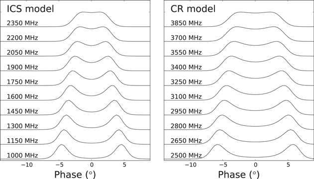
where the factor  represents the photons' dispersion while spreading outwards. The simulation results are shown in Figure 14, revealing that the profile contracts while the frequency increases. Of course, the simulated evolution of the profile with frequency is much faster than that in real data. In fact, this just depends on the functions s and d, and the degree of coherence, which are all uncertain. Since the radiation phase could be transformed to the radiation altitude in the magnetosphere, the phase–frequency mapping of the pulse profile could correspond one-to-one to the radiation spectrum of different points on the magnetic field line at different heights. Furthermore, the energy spectrum of particles at different height could be obtained. In this simulation, the functions s and d describe the evolution of the particle spectrum with height. Thus, the simulated profile evolution can of course always be roughly adjusted to be similar to that of the real data as appropriate functions and degree of coherence are used. In fact, any centrosymmetric profile could be obtained. Then, in Figure 14, only two exemplary results are shown, which show different speeds of profile evolution in different frequency bands.
Figure 14. Simulated multi-frequency profile of a model pulsar under the assumptions pertaining to the ICS and CR models.
Download figure:
Standard image High-resolution image
Footnotes
- 9
- 10
- 11