Functional principal components analysis of workload capacity functions

Abstract

Workload capacity, an important concept in many areas of psychology, describes processing efficiency across changes in workload. The capacity coefficient is a function across time that provides a useful measure of this construct. Until now, most analyses of the capacity coefficient have focused on the magnitude of this function, and often only in terms of a qualitative comparison (greater than or less than one). This work explains how a functional extension of principal components analysis can capture the time-extended information of these functional data, using a small number of scalar values chosen to emphasize the variance between participants and conditions. This approach provides many possibilities for a more fine-grained study of differences in workload capacity across tasks and individuals.

Introduction

From simple experiments with multiple stimulus dimensions to complex multitasking environments, changes in cognitive processes due to increases in workload are important in many areas of cognitive psychology. To assess the effect of workload, a standard approach is to measure performance on each part, such as a single stimulus dimension or a single subtask, and then compare it with performance when all components are present. Often, the analysis of these data is limited to a qualitative judgment of whether performance on each individual part is better than, worse than, or the same as when all components are present. While informative, this measure is relatively limited, particularly when attempting to compare workload across different combinations of parts. In this article, we discuss the workload capacity coefficient, C(t) (Townsend & Nozawa, 1995; Townsend & Wenger, 2004). This rigorous, model-based measure of processing efficiency is unlike the same, better, or worse judgment from traditional workload analyses in that C(t) is a function of time and can be as complex as the data collected. The additional complexity of the measure offers advantages over the traditional measures, but it can also be overwhelming; it can be preferable to describe data in terms of a few summary variables. The focus of our present work is the application of a functional principal components analysis (fPCA) to summarize workload capacity coefficient data with a small number of variables while preserving the largest amount of information contained in those data.

The basic idea of workload capacity is to compare performance with a common baseline model, the unlimited-capacity, independent, parallel model (UCIP). To reify this model, consider a task in which the participants must decide whether any stimulus is presented and they can be shown an audio cue, a visual cue, or both simultaneously. The baseline model predicts that performance in the combined condition will be a simple parallel race between the two single conditions. C(t) is a comparison of that predicted performance with the participants’ performance on trials with both audio and visual cues, and it will show whether they were faster or slower than predicted for each observed reaction time. Because the predicted UCIP performance is based on an individual participant and his or her performance in the single-target conditions, C(t) can be used to compare performance across tasks and individuals in a normalized way.

The capacity coefficient has already proven informative in a wide variety of applications. Neufeld, Townsend, and Jetté (2007) demonstrated its application in the study of cognitive functioning of anxiety-prone individuals, as well as with respect to memory search in schizophrenia. In the field of information fusion, Hugenschmidt, Hayasaka, Peiffer, and Laurienti (2010) used capacity analyses as a finer grained evaluation method in the study of multisensory integration. Workload capacity has also been used to analyze age-group differences in visual processing (McCarley, Mounts, & Kramer, 2007), to test implications of various hypotheses on visual selective attention (Gottlob, 2012), and many more disparate avenues of psychological investigation (e.g., Blaha & Townsend, 2008; Donnelly, Cornes, & Menneer, 2012; Ingvalson & Wenger, 2005; Von Der Heide, Wenger, Gilmore, & Elbich, 2011; Yang, Houpt, Khodadadi, & Townsend, 2011). C(t) functions have even been analyzed parametrically using the linear ballistic accumulator model of Eidels, Donkin, Brown, and Heathcote (2010).

The large amount of data contained in capacity functions can be a great boon to research but, at times, can also be somewhat unwieldy. Figure 1 shows some example capacity functions drawn from experimental data. Consider the graph on the left: A purely qualitative analysis would have trouble characterizing either function as exclusively greater than or less than one and would completely miss other interesting aspects of the data, such as the negative slopes of the functions and the distance between them. These aspects can be seen fairly easily with only two functions, but when more conditions and participants are used, as in the graph on the right, we need a more formal method for finding and characterizing the important differences between the functions. This difficulty in comparing large numbers of functions has led to the capacity coefficient being used most often with smaller data sets using only a handful of participants and conditions. To harness the functionality of this measure for experiments involving larger numbers of participants, it would be desirable to have a rigorous way of quantitatively comparing capacity functions.

Fig. 1

Examples showing the difficulty in comparing capacity performance in a solely qualitative way. The left graph shows data from 1 participant in two different conditions in a face recognition task. The right graph, containing data from the string perception task of Houpt and Townsend (2010), shows capacity functions based on median subtracted response times. Line color indicates condition, and line type indicates the participant

In this article, we demonstrate the use of a functional extension of PCA (e.g., Ramsay & Silverman, 2005) for capacity functions. This approach describes the capacity coefficient using a small number of values (often only two or three) while emphasizing the variation in capacity results across individuals and conditions. These values can be used to efficiently and quantitatively compare the data of any number of participants and conditions, allowing the capacity coefficient to be effective in a broader variety of contexts. The next section describes the fundamentals of fPCA, followed by a brief primer on the capacity coefficient. We will then present data collected in a recent psychological study to walk through the specific methods and demonstrate the use of fPCA for capacity analysis.

Functional principal components

As was previously mentioned with regard to workload capacity, using entire functions as pieces of data can provide much greater power than using a point estimate such as the mean. However, analyzing functional data also brings its own challenges. Previously basic properties and relationships such as greater than become messier when functions are compared, and it can be harder to get an intuitive -level feel for high-dimensional data. These issues call for new tools to both explore and analyze functional data. Fortunately, many previously useful techniques can be easily extended to work with entire functions, rather than isolated data points, and considerable work has already been done in this regard.

Ramsay and Silverman (2005) described a variety of these techniques for analyzing functional data (see also Ramsay, Hooker, & Graves, 2009). Our focus here is on the functional adaptation of PCA, which we refer to as fPCA. This procedure lends itself well to the analysis of high-dimensional data, allowing researchers to explore sources of variation as well as hidden invariants in their data. Also, fPCA provides a good feel for the complexity of a data set by establishing how many components are required to adequately describe the entire corpus of results. The main idea is that given a set of functional data, this procedure will return a number of “principal component” functions describing trends in the data and will report how much of the variance in the data can be explained by each one. A piece of functional data can be approximated by a linear combination of these components (which are functions as well), each multiplied by some scalar. This scalar is called the “score” for a particular datum on that component and has a conceptual interpretation of how much of that component is in that datum. Often, these components will have meaningful interpretations, such as a component that emphasizes early values and depresses later ones, and our list of scores will give us an intuitive (yet mathematically justified) understanding of how much this shape is represented in each of our pieces of data (remember, each piece of data is itself a function). To place this discussion on firmer ground, first let us describe the details of fPCA, and then we can proceed to its implementation for describing workload capacity.

The theory behind fPCA is a structural extension of standard PCA. Here, we give a brief overview of this theory, with a walk-through of an implementation of this theory for our purposes following in a later section. The goal is to describe a set of multivariate data using as small a basis as possible. In standard PCA, the number of dimensions of the data is finite, whereas fPCA extends the theory to infinite dimensional data: functions. In place of the finite dimensional vectors that form the basis in standard PCA, fPCA uses basis functions. Thus, each function in the data is described as a linear combination of the basis functions. The goal is to capture the variation in the data by assigning each piece of functional data a vector of weights for a modest number of basis functions. The components are chosen so that these weights will maximally distinguish the data.

When we extend PCA from a multivariate context into the functional domain, the primary difference is that when, formerly, we would sum variable values, we now must integrate function values. Thus, following the notation of Ramsay and Silverman (2005), when finding the first component in the multivariate case, we solve for the weight vector β ₁ in the weighted sum

$$ {f_{i1 }}=\sum\limits_j {{\beta_{j1 }}{x_{ij }}}, i=1,\ldots,N $$

(1)

so as to produce the largest possible mean square ${N^{-1 }}\sum\nolimits_i\,f_{i1}^2$. In this case, x _ij represents the value of dimension j for observation i. This maximization is subject to the constraint that $\sum\nolimits_j\,\beta_{j1}^2=1$. The difference for the functional case is that we are now combining weight and data functions using integration rather than summation:

$$ {f_{i1 }}=\smallint {\beta_1}(s){x_i}(s)ds. $$

(2)

Likewise, we now choose our weight function β ₁ to maximize the continuous analogue of the mean square:

$$ \frac{1}{N}\sum\limits_i {\,f_{i1}^2} =\frac{1}{N}\sum\limits_i {\,\mathop{{\left( {\smallint {\beta_1}{x_i}} \right)}}\nolimits^2} . $$

(3)

Our constraint on the weight function now takes the form $\int {_{{{\beta_1}}}} {(s)^2}ds=1$. These equations are all that are needed to find the first component, but to find any subsequent components, we must ensure that they are orthogonal to all previous components. In the multivariate case, this constraint is represented for the mth component as

$$ \sum\limits_j {\,{\beta_{jk }}{\beta_{jm }}} =0,\forall k<m. $$

(4)

This constraint is also straightforwardly extended to the continuous domain as $\int {_{{{\beta_k}}}} (s){\beta_m}(s)\:ds=0$.

Computationally solving for these component functions can be done in a number of different ways, but in all cases, we must convert our continuous functional eigenanalysis problem into an approximately equivalent matrix eigenanalysis task. The simplest way to do this is to discretize our observed functions by using a fine grid. A perhaps more elegant method is to express our functions as a linear combination of basis functions (such as a Fourier basis). We can now form a matrix of the coefficients for each basis function for each observed function and use that to compute the component functions.

The same techniques for choosing the number of basis functions to represent the data in PCA can be used in fPCA. For example, in many cases, there is a clear “elbow” in the eigenvalues associated with each of the bases, where after the first few eigenvalues, the addition of more bases provides very little additional descriptive power (see Fig. 2 for a scree plot using our data). A more rigorous decision could be made on a point-wise basis using model comparison methods such as AIC (cf. Yao, 2007). Because the eigenvalues give a direct measure of the percent of variance accounted for (Ramsay & Silverman, 2005), this approach allows the researcher to choose the basis that retains large amounts of variance while eliminating bases that account for only small additional amounts of variance.

Fig. 2

A scree plot showing the amount of variance accounted for by each eigenfunction, ordered from highest to lowest

Often, a rotation of the bases is useful in making the components more interpretable, just as in PCA. When a set of components is rotated, it still accounts for the same total amount of variance in the data, but the individual contributions of the components will change. If we form a matrix B whose rows are our selected principal component functions, the goal of a rotation procedure is to find a rotation matrix T that will give us a new matrix of component functions A = TB. Because T is a rotation matrix, the sum of the squared values of A will remain constant across all rotations. One of the most popular methods for picking a rotation matrix is called varimax rotation, which maximizes the sum of the variance of these squared values, thereby forcing them to be strongly positive, strongly negative, or close to zero. This has the effect of choosing component functions that have a more concentrated and, therefore, more visible effect on the data, while still describing the same total amount of variance with the chosen number of components. This strategy is perhaps even more important for fPCA, since continuous component functions can have complicated effects spread out across the time domain. Concentrating the effects of these components into smaller regions makes it easier to identify the salient features in the data.

An additional step that is often necessary when conducting an fPCA is to register the data so that they can be compared across the same time frame. In some applications, this just means subtracting the median time from all data points, but in other applications, it might also be appropriate to stretch or shrink the time scales of individual data functions so that they all begin and end at the same time. Often, it is also beneficial to smooth the functional data, especially if the function is based upon a relatively small amount of data. In this case, as with any application of smoothing, precautions should be taken to avoid over-smoothing and flattening out important features in the data. These decisions will depend on the kind of data being analyzed and the goals of the analysis. More specific guidelines have been discussed by Ramsay and Silverman (2005).

The capacity coefficient

The workload capacity coefficient (Houpt & Townsend, 2012; Townsend & Nozawa, 1995; Townsend & Wenger, 2004) is a functional measure based upon a comparison of observed performance with the predicted performance of a baseline model. The baseline model assumes unlimited-capacity, independent, parallel processing of each of the information sources. In brief, this is a model where separate sources of information are processed simultaneously (in contrast to serial processing) and without influencing each other. The unlimited-capacity assumption means that each individual channel is processed at the same speed regardless of how many other channels are also being processed (but the system as a whole might still slow down with increased workload if exhaustive processing is required).

The basic idea is to estimate how fast a participant might respond when all sources are present if he or she followed the baseline model assumptions. This estimate is based on his or her response times for each source of information when all other sources are absent. Those times can be combined to determine how long the baseline model will take to process all sources at once, which is then compared with how quickly the participant actually responds in that condition. The result is then a measure of performance targeted at how well the participant uses the sources together, controlling for variations in performance due to the possibly unequal difficulty of each of the sources.

Formally, under the assumption of the baseline model, performance when all sources are processed together is equal (in the sense outlined below) to the summed performance of each source presented in isolation. In particular, if the participant can respond as soon as any one of the sources is completely processed (i.e., an “OR” stopping rule), the probability that he or she has not finished by time t is the product of the probabilities that each source is not yet completed. In terms of the cumulative distribution function, $F(t)=\Pr \left\{ {T\leq t} \right\},$

$$ 1-{F_{UCIP-OR }}(t)=\prod\limits_{i=1}^m\,\left( {1-{F_i}(t)} \right), $$

(5)

where F _i (t) denotes the processing of each of the m sources in isolation. If the participant responds only when he or she has processed all sources of information (i.e., an “AND” stopping rule), the probability of finishing is the product of the probabilities that each source is finished,

$$ {F_{UCIP-AND }}(t)=\prod\limits_{i=1}^m\,{F_i}(t). $$

(6)

Taking the log transform of Eqs. 5 and 6 gives this relationship in terms of the cumulative hazard function (a measure of how much work has been done by a certain time) and the cumulative reverse hazard function (which can be thought of as a measure of how much work is left to be done), respectively:

$$ {H_{UCIP-OR }}(t)=\sum\limits_{i-1}^m {{H_i}(t)} $$

(7)

$$ {H_{UCIP-OR }}(t)=\sum\limits_{i-1}^m {{K_i}(t)} $$

(8)

Houpt and Townsend (2012) showed that using the Neslon–Aalen estimator for the cumulative hazard function, one can obtain an unbiased and consistent estimator of the baseline model performance. Let T _j be the jth element of the ordered set of response times for the condition of interest and Y(t) be the number of responses that have not yet occurred. The Neslon–Aalen estimator for the cumulative hazard function is given by

$$ \widehat{H}(t)=\sum\limits_{{{T_j}\leq t}} {\frac{1}{{Y\left( {{T_j}} \right)}}} . $$

(9)

The estimate of the baseline cumulative hazard function for OR processing of m sources and the estimator of its point-wise variance given in Houpt and Townsend (2012) are

$$ {{\widehat{H}}_{UCIP }}(t)=\sum\limits_{i=1}^m {\sum\limits_{{T_{{_j}}^{(i)}\leq t}} {\frac{1}{{{Y^{(i) }}\left( {{T_j}^{(i) }} \right)}}} } $$

(10)

$$ \mathrm{VAR}\left[ {{{{\widehat{\mathrm{H}}}}_{\mathrm{UCIP}}}} \right]\left( \mathrm{t} \right)=\sum\limits_{{\mathrm{i}=1}}^m {\sum\limits_{{T_{{_j}}^{(i)}\leq t}} {\frac{1}{{{{{\left( {{{\mathrm{Y}}^{{\left( \mathrm{i} \right)}}}\left( {{{\mathrm{T}}_{\mathrm{j}}}^{{\left( \mathrm{i} \right)}}} \right)} \right)}}^2}}}.} } $$

(11)

Houpt and Townsend (2012) also derived analogous estimators for AND processing. With the same notation and G(t) equal to the number of responses that have occurred by time t,

$$ \widehat{K}(t)=\sum\limits_{{{T_j} > t}} {\frac{1}{{G\left( {{T_j}} \right)}}} $$

(12)

$$ {{\widehat{K}}_{UCIP }}(t)=\sum\limits_{i=1}^m {\sum\limits_{{T_{{_j}}^{(i) } > t}} {\frac{1}{{{G^{(i) }}\left( {{T_j}^{(i) }} \right)}}} } $$

(13)

$$ \mathrm{VAR}\left[ {{{{\widehat{\mathrm{K}}}}_{\mathrm{UCIP}}}} \right]\left( \mathrm{t} \right)=\sum\limits_{{\mathrm{i}=1}}^m {\sum\limits_{{T_{{_j}}^{(i) } > t}} {\frac{1}{{{{{\left( {{{\mathrm{G}}^{{\left( \mathrm{i} \right)}}}\left( {{{\mathrm{T}}_{\mathrm{j}}}^{{\left( \mathrm{i} \right)}}} \right)} \right)}}^2}}}.} } $$

(14)

The capacity coefficient for OR processes (when processing terminates as soon as any source is processed) was originally defined by Townsend and Nozawa (1995). With $\widehat{H}$ indicating a cumulative hazard function estimated from a participant’s response times in a particular condition, i indicating a condition in which the participant responds only to source i, and r indicating the condition in which all sources of information are present,

$$ _{\mathrm{OR}}(t)=\frac{{{{\widehat{H}}_r}}}{{{{\widehat{H}}_{UCIP }}}}=\frac{{{{\widehat{H}}_r}}}{{\sum\nolimits_{i=1}^m\,{{\widehat{H}}_i}(t)}}. $$

(15)

The cumulative hazard function can roughly be interpreted as the amount of work completed by a given time (e.g., Townsend & Ashby, 1978). If a participant has more work completed by a particular time when all sources are present than would be predicted by the baseline model, the capacity ratio would be above one. This case is referred to as super-capacity. If the participant has completed less work when all sources are present than what would be predicted by the baseline, the ratio would be below one, referred to as limited capacity.

Townsend and Wenger (2004) defined the analogous measure for AND process (when processing terminates only when all sources are processed) as

$$ _{\mathrm{AND}}(t)=\frac{{\mathop{\widehat{K}}\nolimits_{UCIP }}}{{\mathop{\widehat{K}}\nolimits_r}}=\frac{{\sum\nolimits_{i=1}^m\,{{\widehat{H}}_i}(t)}}{{\mathop{\widehat{H}}\nolimits_r}}. $$

(16)

The cumulative reverse hazard function has the opposite interpretation of the cumulative hazard function. The larger the magnitude of the cumulative reverse hazard function, the more work there is left to be done. Thus, to maintain the interpretation that values of the capacity ratio above one are better than baseline, the ratio is inverted relative to Eq. 15. It can be intuitively seen why these different stopping rules require different capacity formulations. In an OR task where any single source is sufficient to respond, we expect performance to get faster as more sources are added. If, however, all sources need to be completed to respond, as in an AND task, we expect to see participants slow down as more items are added. The above equations ensure that these two different tasks are placed on equal footing such that they can be compared with one another.

Implementation

In this section, we describe the steps involved in performing an fPCA on capacity data by using as an example the data from Tipping and Bishop (1999). These data were collected to get a response-time-based measure of the word superiority effect: the finding that letters are processed more accurately when they are part of a word than when they are presented in isolation (Reicher, 1969; Wheeler, 1970). We were interested in how the processing capacity for identifying a string of four characters would vary as a function of the familiarity of the characters and the particular string. Thus, we used words (W), pseudowords (P), random consonant sequences (R), upside-down nonwords (U), and unfamiliar (Katakana) characters (K). To eliminate the extra probabilistic information available in a word context, each version of the task had a single target string and four distractor strings in which a single character changed in one of each of the positions. For example, in the word condition, the target was “care,” with distractors “bare,” “cure,” “cave,” and “card.”

Each version consisted of two parts. First, we measured the participants’ response times to correctly identify the target string from among the four distractor strings. Second, the participants had to distinguish between each pair of characters that differed between the target and a distractor. For example, in the word condition, participants needed to distinguish between “bare” and “care”; in the second part, participants were required to distinguish between “b” and “c.” Likewise, participants performed the single-letter task for the other three characters as well. Capacity was then computed as a ratio of full-string performance to the sum of each of the four single-character conditions. To correctly identify the target string, a participant needed to check each character in the string, so this was an AND task. Thus, we used the AND capacity coefficient (Eq. 16) composed of reverse cumulative hazard functions. We will estimate ${{\widehat{K}}_r}(t)$ from the string conditions and ${{\widehat{K}}_i},i\in \left\{ {1,2,3,4} \right\}$ from each of the single-character conditions. To implement the fPCA, we took the following steps (which can be seen in more detail in our R code, included in the supporting documents):

• 1. Register the capacity curves by shifting the response times for participants in each condition by their respective median target response times in that condition. The location of features of the capacity coefficient can depend on an individual’s overall response times. Some participants may be slower or faster overall, in both single-target and redundant-target conditions. To focus on variations in capacity, we subtract each participant’s median response time across the single and redundant conditions so that the capacity curves will be better aligned across participants.

• 2. Calculate the capacity function for each participant on the basis of the shifted response times. To calculate the OR capacity coefficient, estimate the cumulative hazard function of a participant’s response times to stimuli with all of the sources present, then divide that function by the sum of each of the estimated cumulative hazard functions for that participant’s response times to each of the single-source conditions. To calculate the AND capacity coefficient, sum the estimated cumulative reverse hazard functions for a participant’s response times for each of the single-source conditions, then divide by the estimated cumulative reverse hazard function for all sources present. Uncertainty in the estimate of the capacity coefficient can be quite large for regions of time when there are only a few measured response times. Thus, large deviations of the capacity functions from the mean capacity are less meaningful in these cases. To remove the effect of regions with high uncertainty on the fPCA analysis, we replace the value of each estimated capacity function in regions with high uncertainty. There are at least a couple of possibilities for this value, but we use the average value of the capacity across all functions, so that there will be no effect of the particular capacity function in that region on the analysis. The AND capacity functions for the word superiority data are shown in the right half of Fig. 1.

• 3. Subtract the mean capacity function across participants. This is done in order to focus on the variation across participants. The mean function can be analyzed on its own to examine the absolute level of capacity, but this analysis is concerned with relative performance. Note that this mean is based on the individual calculated functions, and not directly on pooling of the raw (or shifted) response times. The mean function is shown in Fig. 3, and the mean subtracted capacity functions are shown in Fig. 4. These two figures allow for the separate inspection of group-level trends and variability between participants and conditions.

  Fig. 3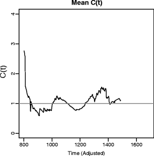

  

  The mean capacity function, averaged across participants and conditions

  Fig. 4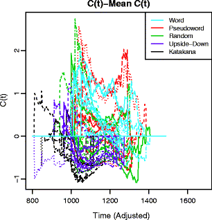

  

  Each of the mean centered capacity functions. Line color indicates condition, and line type indicates the participant

• 4. Calculate the representation of the capacity function in a chosen basis space. Following Ramsay and Silverman (2005), we use quartic B-spline basis with 25 equally spaced knots. There are a number of alternative options at this point, such as using more or unequally spaced knots or another basis. We have not found major effects of these alternatives on the results. Some degree of smoothing is also incorporated into this step, and one should ensure that no major features in the original data are lost in this new representation.

• 5. Determine the basis function that accounts for the largest amount of variance in the data from the chosen basis space, subject to the constraint that the integral of the square of the function is 1 (following Eq. 2–4). The top panel of Fig. 5 shows this component’s effect on the mean function on the left and relative to the mean in the center. Using a finite basis space, this step and the following two can be performed by finding the eigendecomposition of the matrix of coefficients describing each capacity function. Just as in multivariate PCA, the eigenvalues correspond to the proportion of variance accounted for by each eigenfunction. The eigenfunctions in the new space are those functions resulting from the linear combination of the original basis functions with weights given by the eigenvectors.

  Fig. 5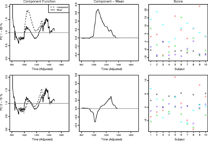

  

  The first three principal components of the capacity functions. The left column shows the component functions, weighted by the average magnitude of the factor score, compared with the mean. The middle column shows the component function weighted by the average magnitude of the factor score. The third panel shows the factor scores for each participant’s capacity function in each version of the task (word, pseudoword, random letters, upside down, and Katakana)

• 6. Find the basis function that accounts for the largest amount of variance in the data, subject to the constraints in Step 4 and orthogonal to the already chosen bases.

• 7. Repeat Step 4 until the desired number of bases has been chosen.

• 8. Apply a varimax rotation to the space. As was stated above, the total variance accounted for does not change with a rotation of the basis; however, by using a varimax rotation, the loading values are forced to be more extreme. As in multivariate PCA, the varimax rotation often leads to better discriminability across participants and more interpretable principal functions. Figure 6 shows the basis functions after a varimax rotation.

  Fig. 6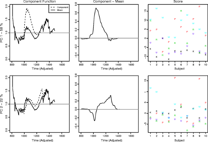

  

  The first three principal components of the capacity functions after a varimax rotation of the basis. The left column shows the component functions, weighted by the average magnitude of the factor score, compared with the mean. The middle column shows the component function weighted by the average magnitude of the factor score. The third panel shows the factor scores for each participant’s capacity function in each version of the task (word, pseudoword, random letters, upside down, and Katakana)

We now have a set of n basis functions to describe the variance between our capacity functions, and for each participant in each string type (word, nonword, etc.), we have n weight values describing how much of each component is needed to describe their performance. These weights themselves can be taken as a low-dimensional description of a participant’s capacity in relation to the group.

fPCA for word superiority

This approach offers a new and interesting perspective on the data from Houpt and Townsend (2010). Before the varimax rotation (Fig. 5), the first principal function indicates that the most variation across capacity functions is accounted for by an overall increase (or decrease for negative factor scores) across time. This function has a larger magnitude at earlier times, indicating that variation tapers off with increasing time. The second principal function indicates that a change of slope is the second most important source of variation: Higher factor scores lead to more positive slopes of the capacity coefficient. Note that, even before the varimax rotation, there are clear differences in the factor scores across conditions.

Roughly the same qualitative form is preserved for the first two principal functions after the varimax rotation (Fig. 6). The first component relates to a general increase (or decrease) of the capacity coefficient, and the figure on the right showing the scores gives a clear indication that words and pseudowords are processed more efficiently than in the other conditions. Nearly all participants had their highest scores on the first component for words and pseudowords and their lowest scores on upside-down nonwords and unfamiliar characters, although there were large individual differences in overall magnitude and the spread between conditions. Another interesting difference highlighted in this figure is that the scores for random consonant sequences were scattered across participants, sometimes appearing at or near the top of that participant’s performance, and sometimes at the bottom.

The second component indicates a change in the slope of the function, lowering capacity for early times and elevating it for later responses. The scores on this component are less consistent across participants, so they may be an indicator of important individual differences. Participants 6 and 9 have high scores for pseudowords, with participants 1 and 2’s scores for words being slightly lower. The majority of the remaining scores are, at most, half the magnitude of those four highest scores.

While the first component is easily interpretable in terms of the underlying cognitive processes, the slope change indicated by the second component is more difficult to understand. Due to the lack of appropriate tools, assessment of the capacity functions has been limited to overall higher-versus-lower comparisons up to now, so there has been little to no theoretical work on the more complex properties. One of our goals with fPCA is to begin to explore the possible connections between functional-level properties of the capacity coefficient and attributes of the underlying cognitive processes.

Discussion

Although using entire functions as pieces of data allows a researcher to retain more power for analyses, functions can be more difficult to interpret or describe. Functional principal components analysis, or fPCA, provides a mathematically rigorous way of representing functional data in a finite dimensional way. It offers the advantage of allowing the researcher to choose the number of components included so as to account for the desired amount of variance and selects these components in such a way as to maximally describe the differences among the data.

This approach is particularly well suited for doing a workload capacity analysis (Townsend & Nozawa, 1995). Because the capacity coefficient describes changes in efficiency across different reaction times, it is desirable to retain that structure rather than collapsing across all values of time (e.g., taking the mean). There are a number of applications (such as structural equation modeling), however, where functional data cannot be used as an input and the data must be represented by a set of finite values. By using fPCA, we can use the scores for each component to describe the way each participant’s capacity function from each condition varies from the group mean. Each component function will depart from the mean in different ways for different values of time, perhaps emphasizing early times while deemphasizing later ones. This can indicate to a researcher which parts of the capacity function are most useful in distinguishing among observers and/or conditions on a given task.

While fPCA has many advantages, there are some shortcomings that we hope to address in future research. As we have mentioned, little is know about the meaningfulness of the features of the capacity functions. Thus, there may be some principal functions that are clearly an important part of the data, but we may not know how to interpret those functions in terms of cognitive processing. While this is a shortcoming, fPCA is also part of the solution. fPCA can isolate the features that correspond to a particular task or condition. We can then work from there to determine what aspects of cognitive processing in that task or condition gave rise to those features.

Another shortcoming of fPCA, inherited from PCA, is that it is not a probabilistic model by nature. This limits the possibilities for making judgments about the loading values. One possible approach to address this shortcoming may be to generalize probabilistic models such as probabilistic PCA (Tipping & Bishop, 1999) to functions.

This approach to analyzing the capacity coefficient differs in many ways from traditional analyses. Most previous work (e.g., Gottlob, 2012; Hugenschmidt et al., 2010; McCarley et al., 2007; Neufeld et al., 2007) focused on a qualitative comparison with a baseline model: the UCIP model. The coefficient was designed so that the UCIP model would produce a value of one, which means performance on an individual item remains constant across increases in workload (thus, unlimited capacity). Values greater than one are called super-capacity, and values less then one are referred to as limited capacity. This level of analysis says nothing about changes in the function over time and is inconclusive if the function is sometimes greater than one and sometimes less. Variation across time might contain important information regarding performance on a task, and it can now be accounted for through the use of fPCA. Is should be noted, however, that this analysis is intended to complement, rather than replace, more traditional comparisons. This is because fPCA describes how individual capacity functions vary from the mean, and thus in a relative sense, in contrast to the absolute comparisons with baseline. In other words, although this new approach excels at describing differences between participants and conditions, it says nothing about characterizing performance using the traditional labels of limited, unlimited, or super-capacity.

In addition to the capacity coefficient, there are other ways to measure workload capacity. The race model inequality (Miller, 1982) compares true performance with a baseline predicted by a race model that does not assume independence. Another measure used in the literature is the Cox proportional hazard model (e.g., Donnelly et al., 2012). A thorough discussion of these approaches is beyond the scope of this article, although fPCA could also be a useful tool for enhancing either measure.

In conclusion, we have demonstrated an effective new tool, fPCA, for the analysis of capacity data. This tool provides researchers with the flexibility to select their own balance between parsimony and accuracy of representation by choosing how many components to use. Importantly, because these components are functions across time, they can speak to variations of capacity at different reaction times, a depth of analysis unavailable in previous methods. The scores for each component that represent the data in this lower dimensional space are a succinct, data-driven way to characterize the capacity variations between participants or conditions quantitatively, allowing capacity analysis to be implemented in a wider variety of psychological domains.

References

Blaha, L., & Townsend, J. (2008). A Hebbian-style dynamic systems model of configural learning. Journal of Vision, 8(6), 1126–1126.
Donnelly, N., Cornes, K., & Menneer, T. (2012). An examination of the processing capacity of features in the Thatcher illusion. Attention, Perception, & Psychophysics, 74(7), 1475–1487.
Eidels, A., Donkin, C., Brown, S. D., & Heathcote, A. (2010). Converging measures of workload capacity. Psychonomic Bulletin and Review, 17(6), 763–771.
Gottlob, L. R. (2012). Aging and capacity in the same-different judgment. Aging, Neuropsychology, and Cognition, 14(1), 55–69.
Houpt, J. W., & Townsend, J. T. (2010). A new perspective on visual word processing efficiency. In Proceedings of the 32nd annual conference of the cognitive science society.
Houpt, J. W., & Townsend, J. T. (2012). Statistical measures for workload capacity analysis. Journal of Mathematical Psychology, 56, 341–355.
Hugenschmidt, C. E., Hayasaka, S., Peiffer, A. M., & Laurienti, P. J. (2010). Applying capacity analyses to psychophysical evaluation of multisensory interactions. Information Fusion, 11(1), 12–20.
Ingvalson, E. M., & Wenger, M. J. (2005). A strong test of the dual-mode hypothesis. Attention, Perception, & Psychophysics, 67(1), 14–35.
McCarley, J. S., Mounts, J. R. W., & Kramer, A. F. (2007). Spatially mediated capacity limits in attentive visual perception. Acta Psychologica, 126(2), 98–119.
Miller, J. (1982). Divided attention: Evidence for coactivation with redundant signals. Cognitive Psychology, 14(2), 247–279.
Neufeld, R. W. J., Townsend, J. T., & Jetté, J. (2007). Quantitative response time technology for measuring cognitive-processing capacity in clinical studies. In R. W. J. Neufeld (Ed.), Advances in clinical cognitive science: Formal modeling of processes and symptoms (pp. 207–238). Washington DC: American Psychological Association.
Ramsay, J. O., Hooker, G., & Graves, S. (2009). Functional data analysis with R and MATLAB. New York: Springer.
Ramsay, J. O., & Silverman, B. W. (2005). Functional data analysis (2). New York: Springer.
Reicher, G. (1969). Perceptual recognition as a function of meaningfulness of stimulus material. Journal of Experimental Psychology, 81(2), 275.
Tipping, M. E., & Bishop, C. M. (1999). Probabilistic principal component analysis. Journal of the Royal Statistical Society. Series B (Statistical Methodology), 61(3), 611–622.
Townsend, J. T., & Ashby, F. G. (1978). Methods of modeling capacity in simple processing systems. In J. Castellan & F. Restle (Eds.), Cognitive theory (pp. 200–239). Hillsdale, NJ: Erlbaum Associates.
Townsend, J. T., & Nozawa, G. (1995). Spatio-temporal properties of elementary perception: An investigation of parallel, serial, and coactive theories. Journal of Mathematical Psychology, 39(4), 321–359.
Townsend, J. T., & Wenger, M. J. (2004). A theory of interactive parallel processing: New capacity measures and predictions for a response time inequality series. Psychological Review, 111(4), 1003–1035.
Von Der Heide, R. J., Wenger, M. J., Gilmore, R. O., & Elbich, D. B. (2011). Developmental changes in encoding and the capacity to process face information. Journal of Vision, 11(11), 450–450.
Wheeler, D. (1970). Processes in word recognition. Cognitive Psychology, 1(1), 59–85.
Yang, H., Houpt, J. W., Khodadadi, A., & Townsend, J. T. (2011). Revealing the underlying mechanism of implicit race bias. In Midwestern cognitive science meeting. East Lansing, MI.
Yao, F. (2007). Functional principal components analysis for longitudinal and survival data. Statista Sinica, 17, 965–983.
Author Note
This work was supported by NIH-NIMH MH 057717-07 and AFOSR FA9550-07-1-0078 awarded to J.T.T.
Author information
Authors and Affiliations
Corresponding author
Rights and permissions
About this article
Cite this article
Burns, D.M., Houpt, J.W., Townsend, J.T. et al. Functional principal components analysis of workload capacity functions. Behav Res 45, 1048–1057 (2013). https://doi.org/10.3758/s13428-013-0333-2
Published:
Issue Date:
DOI: https://doi.org/10.3758/s13428-013-0333-2