
Abstract
The multiple-look notion holds that the difference limen (DL) decreases with multiple observations. We investigated this notion for temporal discrimination in isochronous sound sequences. In Experiment 1, we established a multiple-look effect when sequences comprised nine standard time intervals (S) followed by an increasing number of comparison time intervals (C), but no multiple-look effect when one trailing C interval was preceded by an increasing number of S intervals. In Experiment 2, we extended the design. There were four sequential conditions: (a) 9 leading S intervals followed by 1, 2, …, or 9 C-intervals; (b) 9 leading C intervals followed by 1, 2, …, or 9 S intervals; (c) 9 trailing C-intervals preceded by 1, 2, …, or 9 S-intervals; and (d) 9 trailing S-intervals preceded by 1, 2, …, or 9 C-intervals. Both the interval accretions before and after the tempo change caused multiple-look effects, irrespective of the time order of S and C. Complete deconfounding of the number of intervals before and after the tempo change was accomplished in Experiment 3. The multiple-look effect of interval accretion before the tempo change was twice as big as that after the tempo change. The diminishing returns relation between the DL and interval accretion could be described well by a reciprocal function.
Introduction
Our aim in the present study was to examine discrimination between tempi of isochronous sound sequences comprising empty time intervals delimited by clicks as a function of sequence length. Initially, time discrimination was mainly studied using the classic two-duration discrimination paradigm (see Allan, 1979, for an overview), but, subsequently, more studies investigated time discrimination in or between sound sequences (e.g., Blaschke, 2009; Fraisse, 1967; Friberg & Sundberg, 1995; Grondin, Bisson, & Gagnon, 2011; Halpern & Darwin, 1982; Hibi, 1983; Hirsch, Monahan, Grant, & Singh, 1990; Jones & Yee, 1997; Lunney, 1974; Madison & Merker, 2002; Michon, 1964; ten Hoopen et al., 1994; Yee, Holleran, & Jones, 1994). Some of these studies investigated how the difference limen (DL)Footnote 1 for the tempo difference between two isochronous sequences depends on tempo, often expressed by its inverse: interonset interval (IOI) or stimulus onset asynchrony (SOA).Footnote 2 Other studies investigated whether the DL for anisochrony within an otherwise isochronous sequence is affected by tempo and/or whether the sequential position of temporal perturbation of a sound marker affects the DL. Another study investigated whether the DL for anisochrony in tone sequences is smaller than that in speech. We are rather interested in whether and how the DL for discriminating tempi of isochronous sequences depends on the number of time intervals in the sequences. The notion that multiple observations, in this case of interval durations, might decrease the DL (thus, increase the temporal sensitivity) is called the multiple-look notion, or sometimes repeated-look notion.
The structure of the present article is as follows: First, we will discuss studies that explicitly or implicitly investigated the multiple-look notion as regards time discrimination. Second, we will sketch two preliminary studies on multiple-look effects from our laboratory. Third, we present evidence that time discrimination in auditory sequences differs fundamentally between relatively fast sequences (SOA < 250 ms) and slower sequences (SOA > 250 ms), because this difference might interact with the multiple-look process. Fourth, three experiments will be presented in which the tempo of the sequences, the number of intervals in the sequences, and the time order of standard (S) and comparison (C) sequences were systematically varied. Last, in the General discussion section, we will compare the "reciprocal diminishing returns model" that we derived from our experiments with the seminal "multiple-look model" (Drake & Botte, 1993) and the "generalized multiple-look model" (McAuley & Miller, 2007; Miller & McAuley, 2005).
Drake and Botte (1993), in Experiment 1 of their influential study, utilized an adaptive psychophysical procedure to establish the DL as a function of: (a) the number of empty time intervals in a sequence of short tones, and (b) the tempo of the sequence. In each trial of the adaptive procedure, participants heard two isochronous sequences separated by twice the SOA, both sequences containing the same number of intervals (either 1, 2, 4, or 6), and the listeners had to indicate whether the first (S) or second (C) sequence was faster (thus, notice that the numbers of intervals in S and C were completely confounded). The SOA was varied from 100 to 1,000 ms in steps of 100 ms, and one more SOA of 1,500 ms was added. Drake and Botte found that tempo sensitivity increased significantly when the number of intervals in the sequence increased from 1 to 2, and from 2 to 4. However, sensitivity did not further increase from 4 to 6 intervals. This pattern was found at all SOAs except at 1,500 ms, where there was no further sensitivity improvement after the first extra look (2 intervals). Drake and Botte stated that, “The multiple-look strategy probably involves the creation of a memory trace of the average duration and the degree of dispersion of the intervals in the first sequence heard by the subject. The intervals in the second sequence would be compared with this ‘average’ memory trace. Thus, the more intervals in the first sequence, the more precise would be its memory trace and the greater would be the sensitivity" (p. 284). The authors proposed that the tempo DL at N intervals in the sequences could be predicted from the observed DL for discriminating between two single time intervals by the equation:
Panissal-Vieu and Drake (1998)Footnote 3 summarized their study as follows: “In a 2AFC paradigm, trained listeners identified the slower of two isochronous sequences. The number of intervals was varied in either the first or second sequence, with the temporal window saturated in the other sequence.” (p. 2849). The authors meant by saturation that the multiple-look process works within a limited temporal window providing sufficient information to extract a stable temporal memory trace and that additional information outside this window does not further improve tempo sensitivity. Their aim was to distinguish between two alternatives: Either the increase of the number of intervals in the first sequence (S) is more important (to build a more reliable memory trace), or the increase of the number of intervals in the second sequence (C) is more important (to improve the comparison process). Another aim was to investigate whether the size of the saturated window changed with tempo.
In their first experiment, the number of intervals in S was increased one by one to determine at which number the sensitivity was optimal. By optimal, the authors meant no further significant increase of sensitivity; that is, sensitivity is saturated. The second sequence (C) contained a fixed number of intervals clearly beyond the optimal number; thus, C was saturated. The results showed that the numbers of intervals in S to reach optimal sensitivity were 5, 3, and 3 at 100-, 300-, and 500-ms SOA, respectively. In their second experiment, the roles of S and C were reversed: S contained a fixed optimal number of intervals, and the number of intervals in C was increased one by one. The results showed that the numbers of intervals in C to reach optimal sensitivity were 3, 3, and 3 at 100-, 300-, and 500-ms, SOA, respectively. Panissal-Vieu and Drake concluded that: "These results suggest a buildup of a stable and accurate memory trace during the first sequence which is subsequently compared with the first two intervals of the second sequence" (1998, p. 2849). Thus, the authors did not fundamentally change Drake and Botte's (1993) initial multiple-look model, but they asserted to have refined the model by establishing the widths of the time windows, necessary for a saturated multiple-look process. To us, it is remarkable that the authors did not mention to have partly deconfounded Drake and Botte's design.
Whereas Drake and Botte (1993) and Panissal-Vieu and Drake (1998) observed clear multiple-look effects, a null effect was reported by ten Hoopen et al. (1995). In their Experiment 1, a constant method was used that required the participants to judge whether the last interval of short click sequences that functioned as comparison interval (C) was shorter or longer than the duration(s) of either 1, or 2, or 3 immediately preceding S intervals. The expectation was that an increasing number of S intervals should yield a clearer memory trace of the preceding time interval(s) with which the final interval had to be compared. The base SOAs were varied between 50, 100, 200, and 400 ms. However, four Page tests for ordered alternatives (Siegel & Castellan, 1988), one at each SOA, revealed that there was no significant decrease of the DL with an increasing number of preceding S-intervals; thus, no multiple-look effect was observed.
Grondin (2001a) examined the multiple-look notion for time discrimination in the visual modality. Nevertheless, we summarize Grondin's (2001a) study because he contrasted two types of visual temporal sequences: continuous and discontinuous. In the continuous condition, he presented sequences like those of ten Hoopen et al. (1995), thus comprising 2, 3, or 4 empty time intervals (marked by flashes), of which the last interval functioned as C. Grondin’s discontinuous condition contained two isochronous sequences, separated by two SOAs, such as in Drake and Botte (1993). Both sequences of flashes had the same number of intervals (1, 2, or 3), the first sequence was S, and the second one was C. Grondin ascertained a multiple-look effect in the discontinuous condition at all base SOAs (150, 300, 600, and 900 ms), which replicates Drake and Botte's finding for the visual modality. In the continuous condition, however, no multiple-look effect could be observed at the two shortest SOAs, thus replicating ten Hoopen et al.'s auditory null effect for the visual modality.
Ivry and Hazeltine (1995) investigated how temporal variability increased with duration, and whether time perception and time production used a common timing mechanism. Relevant to the present study is that the results of their Experiments 1, 2, 3 suggested that variability in time discrimination tasks was lower with multiple presentations of the standard interval. Because methodology and participants varied between their Experiments 1, 2, 3, they performed a systematic test on the issue in their Experiment 4, of which we only discuss the perceptual part. The authors distinguished between continuous and discontinuous conditions, like Grondin (2001a) did, but their stimuli were auditory, and they used one base SOA of 500 ms. There was either 1, or 4, S intervals preceding the C interval, which was shorter or longer than S to different extents. In the discontinuous condition, S and C were separated by 900, 1,000, or 1,100 ms, and in the continuous condition, S and C were contiguous. The authors established the temporal variability in these four treatment combinations (1 vs. 4 S-intervals × Discontinuous/continuous) by means of an adaptive psychophysical procedure. The results were clear: Temporal variability was less when four S intervals led the sequence as compared with one leading S. Thus, the multiple-look notion was supported, both for the continuous and discontinuous conditions.
Another relevant study is that of McAuley and Kidd (1998). In their Experiment 3, S and C were two- and four-tone isochronous sequences delimiting 1 and 3 empty time intervals and the S–C combinations were 1–1 and 3–3 intervals. There were four base SOAs of 100, 400, 700, and 1,000 ms. Listeners heard S, followed by two comparisons (C1 and C2) of which one was faster or slower than S, and they had to indicate whether C1 or C2 differed from S. The conditions were discontinuous: The interpattern intervals between S and C1, and between C1 and C2 were twice the base SOA. McAuley and Kidd found a clear multiple-look effect. The absolute DLs (ms) at the SOAs of 100, 400, 700, and 1,000 ms were, respectively, 9, 10, 12, and 17 ms smaller in the 3-interval condition than those in the 1-interval condition.
In a more recent study from McAuley's laboratory, Miller and McAuley (2005) stated that in Drake and Botte (1993), Grondin (2001a), and McAuley and Kidd (1998), the number of intervals in S and C were covaried. To quote the authors, “That is, the multiple-interval advantage may occur because of multiple intervals in the standard sequence, the comparison sequence, or in both.” (p. 1151). Miller and McAuley proposed a generalized multiple-look model, taking into account the conceivable contributions of S and C, by extending Drake and Botte’s model (Eq. 1) to:
In this model, the relative DLs depend inversely on the square roots of N1 (the number of intervals in S), and N2 (the number of intervals in C). The weight parameter w can be either 1 when only S determines the DLs (then the model boils down to Drake and Botte's Eq. 1) or 0 when only C determines the DLs. If w takes a value in between 1 and 0, both S and C contribute to the DLs in a weighted combination.
Miller and McAuley (2005) tested their generalized multiple-look model by independently crossing the number of intervals in S (one or three intervals) and C (one or three intervals). The four pattern conditions (one–one, one–three, three–one, and three–three) were discontinuous, the time lapse between S and C was twice the base SOA, which was 500 ms in their Experiment 1. The participants had to judge whether C was slower or faster than S. It turned out that increasing the number of S intervals from 1 to 3 did hardly or not lower the DL, whereas increasing the number of C intervals from 1 to 3 clearly did. The mean DLs for the patterns 1–1, 1–3, 3–1 and 3–3 were 22, 16, 21, and 15 ms, respectively. The null result (no multiple-look effect) of S-interval accretion from 1 to 3 when followed by 1 C interval observed by Miller and McAuley for discontinuous sequences replicates the null effect found by ten Hoopen et al. (1995) for continuous sequences.
Miller and McAuley (2005) argued that the participants may have built up a stable memory trace for the single SOA used (500 ms), which eliminates the advantage of multiple observations. They tested this argument in their Experiment 2 by varying the SOA of S between 400, 500, and 600 ms, trial by trial. As hypothesized, the authors observed that not only the increase of C intervals, but also the increase of S intervals lowered the DL values. Averaged over the three SOAs, the DLs for the patterns 1–1, 1–3, 3–1, and 3–3 were 40, 32, 33, and 23 ms, respectively. Thus, increasing S from 1 to 3 intervals reduced the DL on average by 8 ms, and increasing C from 1 to 3 intervals reduced the DL on average by 9 ms. In a subsequent study, McAuley and Miller (2007) could replicate the result that increasing the number of intervals in S as well as in C improved temporal sensitivity if the SOA roved between trials.
We will now briefly describe two preliminary studies done in our laboratory to investigate whether multiple-look effects can be demonstrated in continuous sequences. We did an experiment in which the number of preceding S intervals was fixed at 9 and the number of contiguously following C intervals in the sequence increased from 1 to 5 to 9, and the base SOA was varied between 100 ms and 500 ms. We established the DLs by the method of constant stimuli, which were 9.5 ms (1 C), 6.8 ms (5 Cs), and 6.2 ms (9 Cs) when the SOA was 100 ms; and 16.4 ms (1 C), 9.5 ms (5 Cs), and 9.7 ms (9 Cs) when the SOA was 500 ms. We drew two conclusions: (a) the multiple-look effect can also be found in a continuous condition, and (b) there is a multiple-look effect when going from 1 to 5 C-intervals, but not from 5 to 9 C-intervals.
In a second study, we investigated whether a multiple-look effect can be found in continuous sequences by a different paradigm. So-called "grouped anisochrony" was introduced in isochronous sequences containing four, six, eight, or 10 clicks by equally offsetting all even-numbered clicks from their isochronous positions toward the odd clicks to systematic extents (e.g., \( \left| { } \right| \left| { } \right| \left| { } \right| \to \left| { } \right| \left| { } \right| \left| { } \right| \), where | signifies a click). The base SOAs were 100 ms and 400 ms. Participants judged whether the sequences sounded regular or grouped. From the responses we calculated the d' values, which were 1.36, 1.66, 1.71, and 1.69 at SOA = 100 ms, and the d' values were 1.29, 1.44, 1.45, 1.48 at SOA = 400 ms for the sequences containing 4, 6, 8, 10 clicks, respectively. Thus, we found a multiple-look effect in continuous sequences at both SOAs when the sequence length increased from four to six clicks, thus from three to five intervals. Beyond that, no further increase in sensitivity could be observed, and this accords with the first preliminary study.
In these preliminary studies, the SOAs were varied between a very short value (100 ms) and a longer value (500 and 400 ms) because we were aware of a fundamental difference between discriminating time at fast tempi (SOA < 250 ms) and at slower tempi (SOA > 250 ms). Friberg and Sundberg (1995) and ten Hoopen et al. (1994) showed that the absolute DL (ms) for tempo discrimination remained constant up to an SOA of approximately 250 ms. For SOAs longer than 250 ms, however, the relative DL (%) remains constant. In other words: Weber's law does not hold for SOAs shorter than about 250 ms, but does for longer SOAs. In 1964, Michon already described this hinge: “The graph [Michon’s Fig. 4] indeed suggests the operation of two different mechanisms, which supersede each other at an interval length between 200 and 300 ms” (p. 446). Hibi (1983) reported comparable results and coined the terms "holistic processing mechanism" and "ongoing processing mechanism," though he estimated the SOA-boundary between processing fast and slower sequences to be about 300 ms. Several other behavioral studies reported an auditory time window of about 250 ms (e.g., Cowan, 1984; Guttman & Julesz, 1963; for a survey, see Massaro & Loftus, 1996).
There is also psychophysiological evidence for a sensory auditory time window of about 250 ms. Loveless, Levänen, Jousmäki, Sams, and Hari (1996) analyzed neuromagnetic evoked responses to pairs of identical sounds. When presented at intervals less than 250 ms, the second sound evokes an N100mA with enhanced amplitude at150-ms latency. The authors proposed that the amplitude enhancement reflects a temporal integration process with a time constant of 200–300 ms, and concluded that sound sequences within this window seem to be coded holistically. Tervaniemi, Saarinen, Paavileinen, Davilona, and Näätänen (1994) recorded ERPs to infrequent changes in a pair of closely spaced tones. One of the infrequent changes was omitting the second tone, which elicited a mismatch negativity (MMN) when the tone interval (in the unchanged tone pairs) was very short (40 or 140 ms), but not when this interval was longer (240 or 340 ms). It was concluded that, as reflected by the MMN, two closely spaced tones are integrated into a unitary sensory event when within a temporal window of integration lasting 200–250 ms. Comparable studies (e.g., Ross, Picton, & Pantev, 2002; Winkler, Czigler, Jaramillo, Paavilainen, & Näätänen, 1998; Yabe et al., 2001) reported slightly shorter estimates of temporal window integration (~ 200 ms).
Three experiments will be reported here. In Experiment 1, we extended the design of the first preliminary study by using a finer grading of the range of C intervals, contiguously trailing the nine S intervals. In addition, there is a condition in which one trailing C-interval is preceded by an increasing number of S intervals up to nine. Experiment 2 is an expansion of Experiment 1 in which either S or C leads the sequence and either S or C increases from one to nine intervals; thus, there will be a partial deconfounding of the number of S and C intervals. Another important expansion is independently varying the sequential order of S and C and the sequential order of interval accretion—that is, before or after the tempo change. In Experiment 3, we further refine the design of Experiment 2: The number of intervals before and after the tempo change are varied independently; that is, complete deconfounding is accomplished. The choice of base SOA levels in all three experiments was guided by the aforementioned evidence in the literature for two fundamentally different processes of temporal discrimination. ten Hoopen (1992) proposed: (a) that discrimination in the "holistic" time window (< 250 ms) is based on template matching of temporal positions of time-shifted sound markers and their isochronic base positions, which explains that DLs are not affected by the SOA-value, and (b) that discrimination in the "analytic" ("ongoing processing" as Hibi mmmm(1983) called it) time domain (> 250 ms) appears to be based on the duration differences of time intervals between successive sound markers. It is of interest to know whether the holistic and analytic discrimination processes yield different multiple-look patterns In other words, does sensitivity accrue in the same vein when having multiple looks of temporal position deviations as when having multiple looks of duration differences?
Experiment 1
In our first preliminary study, the sequences started with nine S intervals, and the number of contiguously trailing C intervals increased coarsely from 1 to 5 to 9. In the present experiment, we had a set of patterns in which the leading S part of the sequences was also fixed at nine intervals, but a finer graded sampling of the number of C intervals was applied to establish a more precise curvature of the DL-decrease. There was also a set of patterns à la Grondin (2001a) and ten Hoopen et al. (1995), in which one last C interval was immediately preceded by an increasing number of S intervals. Because Grondin (2001a) and ten Hoopen et al. (1995) found no multiple-look effect (at short SOAs) when the number of S intervals increased from 1 to 2 to 3, we applied a larger range (up to nine preceding S-intervals) to explore whether the effect might emerge then.
Method
Participants
Twenty-four students from different faculties of Leiden University, 20 male and four female, 19–30 years of age, served in the experiment. An audiometer test revealed that they had normal hearing as regards pure tones. They were paid 6.5 Dutch guilders ( ≈ 3 Euro) per hour for their services.
Stimuli and design
The stimuli were continuous sound sequences that comprised two isochronous parts, S and C. There were two sets of sequences: In the first set (Set A), the number of intervals in S was kept fixed at nine, and the number of trailing C intervals varied between 1, 2, 3, 5, 7, and 9. The second set of sequences (Set B) comprised only one C interval (the last one), and the number of intervals in the leading S part varied between 1, 2, 3, 5, 7, and 9. The intervals were delimited by 10-ms square waves with a fundamental frequency of 1 kHz, starting and stopping at zero crossings. Note that there was one pattern, nine S intervals followed by 1 C interval, common to Sets A and B. Thus, there were 2 (sets) × 6 (number of intervals) - 1 = 11 different sequence patterns. Because we varied the SOA of the sequences between 100, 200, 400, and 800 ms, there were \( {4}\left( {\text{SOAs}} \right) \times {11}\left( {\text{patterns}} \right) = {\text{44 patterns in total}} \).
Equipment
The sound patterns (sampling rate 22.050 Hz, 8-bit resolution) were presented by an IBM-compatible PC, generated by a soundcard (Turtle Beach) under control of a MATLAB (v. 5.0) program. This program also controlled the experiment and registered the responses. The sound patterns were presented via a Sony TA-FE700R amplifier to both shells of Beyerdynamics DT990 headphones at a comfortable listening level. Tone audiograms were established by a digital screening audiometer (Madsen Electronics, type DS 6214).
Procedure
We applied the method of constant stimuli to establish the DLs for tempo in the 44 conditions. The SOA ranges by which the values of C deviated from the base SOAs of S, and the step size between the Cs, were chosen on basis of ten Hoopen et al. (1995), and further piloting. For Set A, the C ranges were 88 – 120 ms, 180 – 224 ms, 352 – 436 ms, and 712 – 880 ms for the SOAs of 100, 200, 400, and 800 ms, respectively, with (constant) step sizes between the comparisons of 2, 2, 4, and 8 ms respectively. For Set B, the C ranges were 70 – 136 ms, 170 – 230 ms, 348 – 440 ms, and 704 – 872 ms, with the same step sizes as in Set A. All ranges also contained the C values that equaled the value of the base SOA (0-ms deviation).
Twelve participants were first presented with the 24 conditions in which C was kept fixed at one interval (6 patterns × 4 SOAs), followed by the 20 remaining conditions (5 patterns × 4 SOAs) in which S was fixed at nine intervals. The other 12 participants got the reverse order. The blocked presentation of pattern type was done to keep instructions, which differed between Sets A and B, the same over a long spell. When C was fixed at one interval and the leading S was varied, participants were instructed to indicate whether the last click of the sequence came too early or too late. When S was fixed at nine intervals and C varied between two and nine intervals, participants were required to indicate whether the tempo further onwards in the sequence was faster or slower than the tempo in the beginning of the sequence (see Fig. 1 for a task diagram).

Experiment 1. Task diagram. The Set A sound sequences started with 9 standard time intervals (S) contiguously followed by 2, 3, 5, 7, or 9 comparison time intervals (C). Participants had to judge whether the tempo of the sequence decreased or increased. Two examples are depicted: S = 9, C = 3; and S = 9, C = 9 intervals. The Set B sequences ended with one comparison time interval (C) contiguously preceded by 1, 2, 3, 5, 7, or 9 standard time intervals (S). Participants had to judge whether the last click sound came too late or too early. Two examples are depicted: S = 9, C = 1; and S = 3, C = 1 interval(s)
Within each set (A and B), the orders of the 20 and 24 conditions were counterbalanced, and within each condition, the C values were presented twice in randomized order. Under both instructions, participants could mouse click their judgments (last click early/late, or tempo faster/slower) on one of two buttons on a monitor. After responding, they had to press the enter key to release the next trial. Notice that the SOA remained the same until all trials of a condition had been administered (34, 46, 44, and 46 trials for the 100-, 200-, 400-, and 800-ms SOA conditions, respectively). Participants served individually in a sound attenuating booth, taking the 44 conditions in four sessions, two sessions for each set. The sessions lasted about 2 hr, including three short obligatory breaks. Before starting with Set A and Set B, there were training sessions of about 30 min containing examples of all conditions in those sets.
Results and discussion
For each of the 44 conditions, we gathered 24 (participants) × 2 (replications) = 48 judgments at each C value from which the “last sound too late” and “slower tempo” psychometric curves were established. These 44 curves were fitted in three ways: by the classic z-score transformation and least-squares solution, and by probit and logit transformations, using the maximum likelihood method. The PSEs and DLs for the 44 conditions as estimated by the three analyses hardly differed, and for the remainder, we will use the PSE values and DL values as estimated by the classic analysis. The PSEs at 100, 200, 400, and 800 ms did not differ much from the POEs: On average, the CEs (PSE – POE) were +3, +2, -5, and -18 ms respectively.
The overall pattern in Fig. 2 shows that the mean DL decreased at all SOA values as the number of C intervals, trailing the nine S intervals, increased. The negatively accelerated course of the DL is a clear case of diminishing returns: Each additional C-interval (extra look) yields less improvement in sensitivity. Such a course of diminishing returns is often described by several functions: power, logarithmic, and exponential. However, in the present case, it turned out that the course of the DLs at all four SOAs could be fitted best by a reciprocal function: DLestimated \( \left( {{\text{DLest}}.} \right) = {\text{a}} + \left( {{\text{b}}/{\text{N}}} \right){\text{ms}} \), where parameter a is the horizontal DL asymptote, parameter b is the maximum amount of DL decrease possible, and N denotes the number of C intervals. The coefficients of determination were 0.99, 0.95, 0.98, and 0.95 at the SOAs of 100, 200, 400, and 800 ms. We also calculated the corresponding r 2 s for other functions proposed for diminishing returns: power, 0.95, 0.80, 0.88, 0.93; logarithmic, 0.85, 0.77, 0.85, 0.92; exponential, 0.77, 0.55, 0.63, 0.78. All of these r 2 s were smaller; thus, the reciprocal function appears to explain the variance of diminishing returns best. The reciprocal curves, their regression equations, and the coefficients of determination are inserted in Fig. 2. Take, for example, the equation \( {\text{DLest}}. = {2}.{2} + \left( {{9}.{5}/{\text{N}}} \right) \) at SOA = 100 ms. When there is only one C interval, the estimated DL is the sum of parameters a and b; that is, \( {2}.{2} + {9}.{5} = {11}.{\text{7 ms}} \). When there are two C intervals (N = 2, thus one extra look), the estimated \( {\text{DL}} = {2}.{2} + {9}.{5}/{2} = {6}.{\text{95 ms}} \), and so on.

Experiment 1. Mean difference limens (DLs) as a function of the number of comparison intervals, trailing contiguously after a standard sequence of nine intervals, dependent on stimulus onset asynchrony (SOA). The estimated reciprocal functions, their equations and coefficients of determination (Rsq.) are inserted
It is of importance that we have a continuous condition in which a clear and orderly multiple-look effect emerged, not only at the two fast tempi (SOA < 250 ms), but also at the two slower ones (SOA > 250 ms). Figure 2 further shows that the largest DL decreases occur up to three C intervals, about 6 ms at SOAs of 100, 200, and 400 ms, and about 10 ms at an SOA of 800 ms. Although the reciprocal DL-curves keep of course decreasing, the further gain in sensitivity gets smaller and smaller.
Table 1 displays the mean DLs for the sequences with one last C interval, preceded by an increasing number of S intervals. Contrary to the pattern displayed in Fig. 2, showing a diminishing decrease of the DL with an increasing number of trailing Cs, the pattern in Table 1 does not show such a decrease. Although one could argue that increasing the number of leading intervals in S should improve the memory representation of S from which C has to be discriminated, as was proposed by Drake and Botte (1993), the results defy such a proposal. Thus, the fact that Drake and Botte found a multiple-look effect by increasing the number of S intervals might very probably have been caused by concomitantly increasing the number of C intervals. This conviction is supported by the studies of Miller and McAuley (2005) and McAuley and Miller (2007). These authors showed that when the SOA was held constant over trials, tempo sensitivity did not improve by increasing the number of intervals in S, but rather improved by increasing the number of C intervals. However, when S roved trial by trial between different SOAs, an increase of the number of intervals both in S and C improved tempo sensitivity. Similar results have been reported by Grondin and McAuley (2009).
In the present experiment, there were 24 conditions (4 SOAs × 6 numbers of S-intervals) for the Set B patterns in which one last C interval was preceded by 1, 2, 3, 5, 7, or 9 S intervals. The 24 conditions were counterbalanced over the 24 participants, and because the method of constant stimuli was used, the SOA remained the same until all the trials of a condition were administered (34, 46, 44, and 44 trials for the SOAs of 100, 200, 400, and 800 ms, respectively). Thus, the base SOA of S did not rove trial by trial, but changed only when the next condition started. The experiments just discussed suggest that we did not observe a multiple-look effect for the Set B patterns because of nonroving SOAs (see Table 1). However, for the Set A patterns, in which nine S intervals were followed by an increasing number of C intervals, the 20 conditions were also counterbalanced, and the SOA did not rove either between the trials of a condition. Yet, a clear multiple-look effect emerged (see Fig. 2). Thus, a nonroving SOA cannot explain that the multiple-look effect failed to occur for the Set B patterns. We strongly surmise that the reason is that the Set B patterns had only one final C interval. This was also suggested by Blaschke (2009) in his discussion of the null results reported by Grondin (2001a) and ten Hoopen et al. (1995).
Experiment 2
In Experiment 1, we deliberately chose two different sets of sequences. Set A (nine S intervals, trailed by an increasing number of C intervals), and Set B (one trailing C interval, preceded by an increasing number of S intervals). In this experiment, we discarded the Set B patterns, but added to the Set A patterns its reverse condition of nine last C intervals, preceded by an increasing number of S intervals. This reverse condition is of special importance: Does a multiple-look effect emerge when there is not one last C interval, but nine? To complete this design, we added mirror conditions in which the time order of S and C was swapped. Such a C/S – S/C time order variable makes it possible to determine whether the magnitude of a multiple-look effect, in the event of occurrence, is dependent on interval accretion either in S or C, or whether the magnitude is dependent on interval accretion before or after the tempo-change—that is, irrespective of whether the accretion is in S or C.
Method
Participants
The five participants, between the ages of 18 and 24, one female and four male, were Leiden University students and were either paid or received curriculum credits for their services. No tone hearing deficiencies were detected.
Stimuli and design
The 36 different sound sequence types are given in Table 2. The sound markers had the same characteristics as those in Experiment 1. Because the SOA was varied between 200 and 400 ms, there were 72 different sequences. The factors were: (a) SOA [200 or 400 ms], (b) before/after [accretion of the number of S or C intervals before or after the tempo change], (c) time order [sequences starting with C or S], and (d) interval accretion [1 to 9]. Thus, we had a 2 × 2 × 2 × 9 factorial design.
Equipment
The sound sequences were generated and presented by a basic program running on a Commodore Amiga 500+ computer, which also controlled the experiment and registered the responses. The amplifier, headphones, and audiometer were the same as in Experiment 1.
Procedure
Following Cornsweet (1962), we used a multiple interleaved staircase method to establish the upper limens (UL) and the lower limens (LL) separately, from which the DLs could be calculated. The 144 runs (36 sequence patterns × 2 SOAs × 2 limens) were divided over 24 sextuples. Within each sextuple, the SOAs and limens were balanced, and sequence type was balanced across sextuples. The trials of the six runs of a sextuple were randomized so that any two consecutive trials came from different runs.
When, after hearing a sequence, the participant keyed in “Y” (for “Yes, I do hear a tempo change”), the value of the C intervals was adapted toward the value of the S intervals. When, after hearing a sequence, the participant keyed in “N” (for “No, I do not hear a tempo change”), the difference between the values of the C and S intervals was incremented. The stepsize of this adaptation was held constant at 4 and 6 ms for the SOAs of 200 and 400 ms, respectively.
For the estimation of the ULs, the runs started at 230 and 440 ms for SOAs of 200 and 400 ms, respectively. For the LL estimations, the runs started at 170 and 360 ms for SOAs of 200 and 400 ms, respectively. A “Y” followed by a “N,” and an “N” followed by a “Y,” was registered as a reversal point. After 10 reversal points, a run was finished. After ample training, the participants took individually part in six sessions, and in each session, four sextuples were presented, divided by three short breaks. The six groups of four sextuples were counterbalanced as far as possible. The sessions took approximately 2 hr each and were held on different days in a sound attenuating booth.
Results and discussion
For each of the five participants, we calculated the LLs and the ULs for all 72 sequences by averaging the 10 reversal points of the respective runs, and from these values, we calculated the DLs [DL = (UL-LL)/2]. The DLs were submitted to a repeated measures ANOVA: 2[SOA (200/400 ms)] × 2 [before/after (interval accretion before or after tempo-change)] × 2[time order (C/S or S/C)] × 9 [interval accretion (1 to 9)] × 5 [participants].
We now summarize the main and interaction effects and, where necessary, we corrected the degrees of freedom according to Greenhouse–Geisser. The main effect of SOA was significant, F(1, 4) = 31.89, MSe = 1257.2, p < .005, \( \eta_{\text{p}}^2 = 0.{889} \). The mean DLs at SOA = 200 ms and 400 ms were 16.8 ms and 27.4 ms, respectively. The main effect of before/after was significant as well, F(1, 4) = 19.95, MSe = 325.47, p < .01, \( \eta_{\text{p}}^2 = 0.{842} \). The mean DL before the tempo change was 24.3 ms, and the mean DL thereafter was 19.9 ms. The main effect of interval accretion was significant, F(1.260, 5.042) = 15.62, MSe = 2640.99, p < .009, \( \eta_{\text{p}}^2 = 0.{799} \). The mean DL decreased with increasing number of intervals from 35.3 ms (one interval) to 18.9 ms (nine intervals), supporting the multiple-look notion.
The only main effect that was not significant (p < .50) was that of time order. The mean DLs of C/S and S/C were 22.2 and 22.0 ms, respectively. Although this variable was logically included to complete the design from an experimenter’s point of view, as Table 2 illustrates, it did not affect the discriminative behavior of the listeners. This is understandable in terms of the task requirement: The participants had to detect a tempo difference between the two isochronous parts of the sequences, but had no cues whatsoever which part was C or S.
The interaction effect between SOA and before/after was significant, F(1, 4) = 28.19, MSe = 38.45, p < .006, \( \eta_{\text{p}}^2 = 0.{876} \). At SOA = 200 ms, the mean DLs before and after the tempo change were 18.1 and 15.5 ms, respectively, and at SOA = 400 ms, these values were 30.4 and 24.3 ms. The interaction effect between before/after and interval accretion was significant as well, F(1.437, 5.748) = 9.02, MSe = 904.18, p < .02, \( \eta_{\text{p}}^2 = 0.{692} \). When the interval accretion occurred before the tempo change, the mean DL decreased from 43.2 ms (one interval) to 19.1 ms (nine intervals), whereas the DL decrease after the tempo change was from 27.5 ms to 18.8 ms. None of the other interaction effects reached significance, and only the interaction between SOA and interval accretion bordered on significance (p < .084, Greenhouse–Geisser correction; p < .036, Huynh–Feldt correction).
It is clear from the previous effects that the pattern of results can be best portrayed in terms of the factors SOA, before/after, and interval accretion; hence, we plotted the mean DLs as a function of these three factors in Fig. 3. We fitted reciprocal functions to the observed DLs as a function of interval accretion for the four SOA × Before/After combinations. The inserted curves and their coefficients of determination show that the fits were excellent for the before condition, and were reasonable for the after condition (as in Experiment 1, the reciprocal fits were better than alternative candidates). At both SOAs, the decrease of the before DLs with interval accretion is bigger than the decrease of the after DLs. Thus, the gain in sensitivity by adding more intervals— that is, the multiple-look effect—is greater when interval accretion occurs before the tempo change than when accretion occurs thereafter. In the General discussion section, we will offer an explanation for this difference.

Experiment 2. Mean difference limens, averaged over “standard first” and “comparison first,” for the conditions in which the accretion of the number of intervals is before (squares) or after (circles) the tempo change as a function of stimulus onset asynchrony (SOA). Inserted are the best-fitting reciprocal functions, their regression equations, and the coefficients of determination. DLest. denotes the estimated difference limen
The reciprocal curves seem a clear illustration of the SOA × Before/After interaction; that is, the curves indicate that the mean DL difference between the before- and after-level at SOA = 400 ms is larger than the corresponding mean DL difference at SOA = 200 ms. To analyze this significant interaction further, we ran two 3-way ANOVAs [2 (before/after) × 2 (time order) × 9 (interval accretion)], one at SOA = 200 ms, and the other one at SOA = 400 ms. Although this procedure to test for simple main effects by running subsequent ANOVAs with one factor less is secure for between-subjects designs, applying the procedure to within-subjects designs requires a stricter criterion for the significance of the simple main effects because of the dependence between levels of a factor (in this case, two SOA-levels). Thus, we set the criterion following Bonferroni at 0.05/2 = 0.025. The simple main effect of before/after at SOA = 200 ms (2.6 ms) was not significant, F(1, 4) = 6.604, p < .062, \( \eta_{\text{p}}^2 = 0.{692} \), but the simple main effect of before/after at SOA = 400 ms (6.1 ms) was significant, F(1, 4) = 39.314, p < .003, \( \eta_{\text{p}}^2 = 0.{9}0{8} \).
We also analyzed the other significant interaction (before/after × interval accretion, p < .02) because Fig. 3 illustrates that at accretion levels 6, 7, 8, and 9, the differences between the before and after DLs get extremely small or even negative. For each of the five participants, and at each accretion level (1 to 9), we averaged the DLs over SOA and time order, and applied t tests to inspect which mean before and after DLs at the nine accretion levels differed significantly. The DL differences at accretions 1 to 5 (15.7, 8.4, 4.6, 4.4, and 3.7 ms, respectively) were significant; the five paired-samples t tests (df = 4, two tailed) yielded p values of .025, .02, .02, .015, and .01, respectively. The remaining four DL differences at interval accretions 6 to 9 (0.6, 2, - 0.2, and 0.3 ms, respectively) were not significant; the corresponding p values were 0.44, 0.12, 0.86, and 0.62.
The results of the previous two analyses, (a) no significant simple main effect of before/after at SOA = 200 ms, and (b) no significant differences between before and after levels at the interval accretions beyond five, lead to an important question. Would the simple main effect have been significant if there had been only interval accretions from one to five? We first ran a 2 (SOA) × 2 (before/after) × 2 (time order) × 5 (interval accretion) repeated measures ANOVA to test whether the same significant effects emerged again. The main effects, except for time order, were significant, and the SOA × Before/After and the Before/After × Accretion interactions were significant as well (p < .012 and p < .002, respectively). Thus, again, two Before/After × Time Order × Accretion repeated measures ANOVAs were run, one at 200-ms SOA, and the other one at 400-ms SOA. Given the Bonferroni criterion of .05/2 = .025, the simple main effect of before/after at SOA = 200 ms (4.5 ms) was not significant, F(1, 4) = 8.675, p < .042, \( \eta_{\text{p}}^2 = 0.{684} \), but the simple main effect of before/after at SOA = 400 ms (10.2 ms) was significant, F(1, 4) = 24.856, p < .008, \( \eta_{\text{p}}^2 = 0.{861} \). It is evident that removing the negligible DL differences between the before and after conditions by deleting the accretion levels six to nine from the design increased both simple main effects. Nevertheless, the simple main effect at SOA = 200 ms still did not reach significance, although its p value of .042 closely approached the .025 criterion. Two facts appear to account for this: As Fig. 3 shows, the mean observed DL difference at accretion three is negligible (1.2 ms) and in Experiment 3, we will see and explain that the after DLs at the level of three intervals are often larger than those at two and four intervals. The other fact is the huge between-subjects variance, F(1, 4) = 82.618, p < .001, \( \eta_{\text{p}}^2 = .{954} \); thus, the number of participants we chose appears somewhat meager.
The most important conclusion is that interval accretions before and after the tempo change both produce a multiple-look effect. The proportional effect sizes were calculated by dividing the regression coefficients (parameters b) of the reciprocal before function and the reciprocal after function by the sum of these coefficients. At 200-ms SOA, the proportional sizes were 0.70 and 0.30, and at SOA = 400 ms, the proportional sizes hardly differed from those at 200 ms: 0.73 and 0.27. Again, it appears that the multiple-look process operates similarly on "holistic" and "analytic" temporal discriminations. Notice finally that the design of this experiment—keeping the number of intervals constant either before or after the tempo change and increasing the number of intervals after or before the change—is the same as Panissal-Vieu and Drake's (1998) design.
Experiment 3
In Experiment 2, the numbers of intervals before and after the tempo change were only deconfounded to a small extent. A complete image of the multiple-look effects as a result of interval accretion before and after the tempo change can be obtained only by independently varying all the numbers of intervals before the tempo change with all numbers of intervals thereafter, which is done in this experiment.
Method
Only deviations from the method of Experiment 2 will be described. The same five students from Experiment 2 plus one new participant (a female student of the same age group) served in the experiment. Because Experiment 2 showed that the time order of S and C did not affect the magnitude of the multiple-look effect, we chose for economic reasons, sound sequences that started with an isochronous S, containing 1, 2, 3, 4, or 5 intervals, followed immediately by an isochronous C, also containing 1, 2, 3, 4, or 5 intervals. All combinations were used; thus, there were \( {5} \times {5} = {25} \) different sequence patterns of which the length varied between 2 and 10 intervals. Also for economic reasons, we chose a range from 1 to 5 intervals instead of from 1 to 9 because Experiment 2 showed that: (a) the DLs hardly or do not get smaller beyond five intervals, and (b) the DL differences between the before and after conditions are not significant anymore beyond interval accretion 5. We kept the same SOAs as applied in Experiment 2; thus, there were 5 (S intervals) × 5 (C intervals) × 2 (SOAs) = 50 different sequences. Therefore, the multiple interleaved staircase method comprised 100 runs (50 sequences × 2 limens [LL/UL]), which were divided over 20 quintuples. In each quintuple, the SOAs and limens were balanced as far as possible. The participants took individually part in four sessions, and in each session, five quintuples were presented, divided by four short breaks.
Results and discussion
For each of the six participants, we calculated the DLs in the same way as in Experiment 2. In Fig. 4, we plotted the mean DLs as a function of three factors: (a) sequence lengths [2–6, 3–7, 4–8, 5–9, and 6–10, in Figures 4A–E respectively], (b) SOA [200 or 400 ms, left and right figure panels respectively], and (c) number of intervals [1, 2, 3, 4, or 5] before [B] or after [A] the tempo change. In Fig. 4A, the mean DLs of two sets of five sequence patterns are plotted: of the set BA, BAA, BAAA, BAAAA, BAAAAA, and of the set BA, BBA, BBBA, BBBBA, BBBBBA. Thus, the sequence length in both sets varies from 2 to 6 intervals. In the first set of 5 patterns, the tempo change occurs straight after the first interval (B), and the interval accretion from 1 to 5 is after (A) the tempo change. In the second set, the tempo change occurs just before the last interval (A), and the interval accretion from 1 to 5 is before (B) the tempo change. In each next plot (Figs. 4B to E), the sequence lengths are increased by one interval, ultimately resulting in set BAAAAA, BBAAAAA, BBBAAAAA, BBBBAAAAA, BBBBBAAAAA, and in set BBBBBA, BBBBBAA, BBBBBAAA, BBBBBAAAA, BBBBBAAAAA as depicted in Fig. 4E. Thus, the sequence length in these latter two sets varies from 6 to 10 intervals.


a Experiment 3. Mean difference limens at stimulus onset asynchronies of 200 (left panel) and 400 ms (right panel) for the sequences in which there is one interval before (B) or after (A) the tempo change and the number of A or B intervals increases from one to five. b Experiment 3. Mean difference limens at stimulus onset asynchronies of 200 (left panel) and 400 ms (right panel) for the sequences in which there are two intervals before (B) or after (A) the tempo change and the number of A or B intervals increases from one to five. c Experiment 3. Mean difference limens at stimulus onset asynchronies of 200 (left panel) and 400 ms (right panel) for the sequences in which there are three intervals before (B) or after (A) the tempo change and the number of A or B intervals increases from one to five. d Experiment 3. Mean difference limens at stimulus onset asynchronies of 200 (left panel) and 400 ms (right panel) for the sequences in which there are four intervals before (B) or after (A) the tempo-change and the number of A or B intervals increases from one to five. e Experiment 3. Mean difference limens at stimulus onset asynchronies of 200 (left panel) and 400 ms (right panel) for the sequences in which there are five intervals before (B) or after (A) the tempo change and the number of A or B intervals increases from one to five
We were, of course, interested in whether the mean DLs in each of the 20 systematically ordered sets followed a reciprocal trajectory as a function of interval accretion. If the five consecutive mean DLs in a set could be fitted by a reciprocal function (our arbitrary criterion was a coefficient of determination of 0.75), the drawn curve of the function and its regression equation was inserted in Fig. 4. If a fit did not meet the criterion of r 2 = .75, the five mean DLs in a set were connected by straight lines. At the SOA of 200 ms (Figs. 4A to E, left panels), nine of the 10 DL-trajectories could be fitted reasonably (0.77 and 0.88) or well (0.90 to 0.99) by reciprocal functions. The only case in which no reciprocal function could be fitted was for the set of five patterns BA, …, BAAAAA—that is, the set of shortest sequence lengths (2–6) in which the interval accretion is after the tempo change (see Fig. 4A, left panel, triangle-marked DLs).
At the SOA of 400 ms (Figs. 4A to E, right panels), only six of the 10 DL trajectories could be fitted reasonably (0.75) or well (0.90 to 0.99) by reciprocal functions. For the two sets of shortest sequence lengths 2–6 (set BA, …, BAAAAA, and set BA, …, BBBBBA), no fit could be made (Fig. 4A, right panel). For the sets of longer sequence lengths (3–7 through 6–10), fits could be made if the interval accretion was before the tempo change (Figs. 4B to E, right panels, diamond = marked DLs). When interval accretion was after the tempo change, fits could be made only when the sequence lengths were 5–9 and 6–10 (Figs. 4D and E, right panels, triangle marked DLs). In particular, when the interval accretion was after the tempo change (triangle markers in Fig. 4), and when the sequences were relatively short, there was a clear tendency that the DLs at the odd number of 3 intervals were bigger than those at the even numbers of 2 and 4 intervals. Also, the DLs at the odd number of 5 intervals were sometimes bigger than the DLs at 4 intervals. In a few cases, these tendencies were so strong that no reciprocal fit could be made; thus, an odd–even effect appears not only to be superimposed, but can even override the reciprocal decrease of DLs with interval accretion.
We surmise that the odd–even effect is brought about by subjective rhythmization of isochronous sound sequences (Bolton, 1894). A very common subjective group size is two; the first sound marker of each subjective group seems accented (Fraisse, 1956), and the subjective duration between consecutive groups of two sounds tends to be overestimated (Stetson, 1905). Because three intervals are of course marked by four sounds and five intervals by six sounds, subjective rhythmization generates two or three groups of two sounds. These subjective temporal alterations (subjective time dilation between groups of two, and accentuation of the groups) may have introduced anisochrony in the sequence part trailing the tempo change and have lowered sensitivity of discrimination.
In the greater number of cases in which the reciprocal pattern of DLs was not overridden by the odd–even effect, the slope of the before reciprocal functions is steeper than the slope of the after functions, which implies that the multiple-look effect of interval accretion before the tempo change is stronger. This accords with the results of Experiment 2 (see Fig. 3) in which the proportional multiple-look effects of the before and after accretions were 0.70 - 0.30 at SOA = 200 ms, and 0.73 - 0.27 at SOA = 400 ms. The proportional multiple-look effects in the present Experiment 3 were 0.69–0.31, 0.65–0.35, 0.64–0.36, and 0.68–0.32 at the SOA of 200 ms (note that the proportion could not be calculated for the results shown in Fig. 4A). Thus, on average, the proportional effect was 0.67–0.33. At the SOA of 400 ms, the proportions were 0.66–0.34 and 0.62–0.38 (note that the proportion could not be calculated for the results shown in Figures 4A, B, and C). Thus, on average, the proportional effect was 0.64–0.36. These values do not differ much from those found in Experiment 2. More important, there is hardly a difference between the proportions at the SOAs of 200 and 400 ms, offering still more support that the multiple-look process operates similarly in different time windows (SOA < 250 ms, and SOA > 250 ms). In the General discussion section (subsection “Model of reciprocal diminishing returns”), we will explain why the regression coefficients of the reciprocal functions are much larger when the interval accretion occurs before the tempo change.
In the previous analysis, the positions of the tempo change were fixed in each of the five sets of sequences, and the number of intervals before or after the tempo-change increased. We wondered what the pattern of DLs would look like when the sequence lengths are kept constant, but the position of the tempo change in the sequences varies. Therefore, in a second analysis, we divided the sequences into groups of equal sequence length. The groups of sequence lengths 3, 4, 5, 6, 7, 8, and 9 have 2, 3, 4, 5, 4, 3, and 2 members respectively. The shortest sequence (two intervals) and the longest sequence (10 intervals) can of course not be grouped, because there is only one specimen of each. Figure 5 shows the groups of sequence lengths and the DLs of their members for the SOAs of 200 ms (top panel) and 400 ms (bottom panel). For clarity of inspection, the groups are systematically divided over three horizontal panels.

Experiment 3. Mean difference limens at the stimulus onset asynchrony (SOA) of 200 ms (top panel) and 400 ms (bottom panel) grouped with regard to equal numbers of intervals in the sequences (3, 4, 5, 6, 7, 8, and 9) as a function of the number of intervals before the tempo change. “B” signifies the interval(s) before, and “A” signifies the interval(s) after the tempo change. The mean difference limens of the shortest and longest sequence (BA and BBBBBAAAAA) of the 25 sequence types, not depicted in the figure, were 34.4 and 18.2 ms, respectively, at SOA = 200 ms; and 42.6 and 29.9 ms, respectively, at SOA = 400 ms
Several trends can be observed in the DL patterning within a group, and we exemplify this for the group of patterns with a sequence length of six intervals (middle panels). Tempo sensitivity is worst (DL highest) when the tempo change in the sequence occurs straight after the first interval of the sequence, but there is a big enhancement of sensitivity when the tempo change occurs after the second interval. Compare the DLs of patterns BAAAAA and BBAAAA in the middle panels of Fig. 5. At both SOAs (200 and 400 ms), the DL decreases 12 ms by shifting the tempo change one position further. Another trend is that the sensitivity for a tempo change just before the last interval is higher (DL lower) than for a tempo change straight after the first interval of the sequence, as a comparison of the DLs of patterns BAAAAA and BBBBBA shows. At the SOA of 200 ms, the DL for the latter pattern is 9 ms smaller, and at the SOA of 400 ms, the DL for the latter pattern is 7 ms smaller. Notice further that the sensitivity increases when the tempo change is penultimate. Comparing patterns BBBBBA and BBBBAA shows DL decreases of 5 ms and 6 ms for the latter pattern at the SOAs of 200 ms and 400 ms, respectively.
From the previous inspections of the five patterns having a sequence length of six intervals, it is clear that when the tempo change occurs in the very beginning or the very end of the sequence, sensitivity is worst, and more so for a tempo change in the beginning. Shifting the position of tempo change only one interval more, either forward or backward in the sequence, yields the maximum sensitivity improvement, but the multiple-look effect is bigger when going from BAAAAA to BBAAAA than when going from BBBBBA to BBBBAA. Shifting the position of tempo-change to the middle of the sequence yields the pattern BBBAAA of which the DLs do hardly or not differ from the DLs of their neighbor patterns BBAAA and BBBBAA. Some of these trends exemplified previous can be observed in the other groups as well, depending on sequence length and SOA.
There is one last interesting subset of patterns, namely BA, BBAA, BBBAAA, BBBBAAAA, and BBBBBAAAAA, because this subset is quite similar to the patterns used by Drake and Botte (1993). Recall that their S and C sequences both contained 1, 2, 4, or 6 intervals, but were separated by twice the SOA, the so-called discontinuous condition. Our subset of patterns was continuous and almost covered Drake and Botte's range of intervals (1, 2, 3, 4, 5 vs. 1, 2, 4, 6). Comparing the courses of the DLs with interval accretion in both experiments gives us another opportunity to inspect whether a multiple-look effect can also emerge in a continuous condition. In Fig. 6, we plotted the observed absolute DLs of both studies at the comparable SOAs of 200 and 400 ms as a function of interval accretion and inserted the reciprocal fits and their equations. For Drake and Botte's data (top panel), the reciprocal regressions were significant at the SOAs of 200 ms (p < .029; r 2 = .94) and 400 ms (p < .006; r 2 = .98), as they were in the present study (bottom panel: p < .009; r 2 = .92 and p < .008; r 2 = .93, respectively). As the bottom panel shows, there is a clear multiple-look effect for the continuous condition as well. Note that, although the reciprocal regressions were significant, the bottom panel again illustrates the interference of the odd–even tendency we discussed: DLs at 3 intervals were larger than those at 2 and 4 intervals. Because Drake and Botte skipped the level of 3 intervals (they also skipped 5), the r 2 values of the reciprocal fits to their DLs are somewhat larger than the r2 values of the fits to our DLs. Here, we compared our data with those of Drake and Botte at the shared SOAs of 200 and 400 ms, but in the General discussion section, we will reanalyze their data at the other SOAs they used as well.

Experiment 3. Top panel: Observed mean difference limens (DLs) at stimulus onset asynchronies (SOAs) of 200 ms (circles) and 400 ms (squares) as a function of the number of intervals as reported by Drake and Botte (1993). The estimated reciprocal functions and their equations are inserted. Bottom panel: Observed mean DLs at SOAs of 200 ms (circles) and 400 ms (squares) as a function of the number of intervals as found in the present study. The estimated reciprocal functions and their equations are inserted
General discussion
In Experiment 1, we presented two sets of sequential sound patterns. In the first set, the sequence started with 9 empty time intervals of equal duration, marked by 10 short sounds. This isochronic part functioned as the temporal standard (S), and the stimulus onset asynchronies (SOAs) were 100, 200, 400, and 800 ms. This initial S part of the sequence was followed contiguously by 1, 2, 3, 5, 7, or 9 comparison intervals (C). Participants had to judge whether the tempo in the (total) sequence became faster or slower. The results showed that the DL decreased with increasing C at all SOAs; that is, multiple-look effects were observed. The DL decreases could be fit very well by a reciprocal function \( \left[ {{\text{DLest}}. = {\text{a}} + \left( {{\text{b}}/{\text{N}}} \right){\text{ms}}} \right] \). In the second set of sequential sound patterns, there was one last C interval immediately preceded by 1, 2, 3, 5, 7, or 9 S intervals. Participants had to judge whether the last sound of the total sequence came too early or too late. The DLs did not decrease with an increasing number of preceding S intervals; that is, no multiple-look effects could be observed.
In Experiment 2, there were four sequential conditions: (a) 9 leading S intervals followed by 1, 2, …, or 9 C intervals; (b) 9 leading C intervals followed by 1, 2, …, or 9 S intervals; (c) 9 trailing C intervals preceded by 1, 2, …, or 9 S intervals, and (d) 9 trailing S intervals preceded by 1, 2, …, or 9 C intervals. Of all 36 sequential patterns, the temporal ULs and LLs were measured by an interleaved staircase method at the SOAs of 200 and 400 ms, from which the DLs were calculated. We showed that the following main effects were significant: SOA, interval accretion and before/after (whether interval accretion was before or after the tempo change). There was no main effect of the time order of S and C. We therefore averaged the DLs over C/S and S/C and plotted them against interval accretion (one to nine intervals) as a function of SOA and of whether the accretion was before or after the tempo change. Clear decreases of DL were found at both SOAs. The multiple-look effect of interval accretion before the tempo-change was much larger than that after the tempo change. The DL patterns could be fit by reciprocal functions.
In Experiment 3, we fully deconfounded the numbers of intervals in S and C. The SOAs were 200 and 400 ms, and the number of intervals was varied from 1, 2, 3, 4, to 5, yielding 25 S/C pairings at each SOA. The psychophysical procedure was the same as in Experiment 2. A first detailed analysis showed that the DL decreases with interval accretion could be well accounted for by reciprocal functions in most cases. The multiple-look effect of interval accretion before the tempo change was larger than that after the tempo change. However, in some cases, an odd–even pattern of DLs overrode the reciprocal decrease, probably as a result of subjective rhythmization within the isochronous structure. In a second detailed analysis, we grouped the sequences according to number of intervals—that is, sequence length. In each group, the position of the tempo change varied. The DLs were largest if the tempo-change occurred in the very beginning of the sequence, and second largest if the tempo change was at the very end of the sequence. If the tempo changes occurred at sequence positions in between, the DLs were smallest. In a third and last analysis, we selected sequences that increased in length, but in which the tempo change was halfway (BA, BBAA, BBBAAA, BBBBAAAA, and BBBBBAAAAA) and compared the pattern of DLs with the pattern established by Drake and Botte (1993). Although our sequences were continuous and those of Drake and Botte were discontinuous (B A, BB AA, …), both patterns of DLs were very similar. The diminishing returns reciprocal function also fitted Drake and Botte's DLs very well.
Model of reciprocal diminishing returns
In Experiment 1, we reported that the best-fitting function relating the decrease of DL to the number of looks (N) was: \( {\text{DL}} = {\text{a}} + \left( {{\text{b}}/{\text{N}}} \right){\text{ms}} \). Although the goodness of fit of this reciprocal function was very good (and better than that of common candidates, such as a power function, etc.), it was not so easy to grasp the perceptual reality of the parameters of the reciprocal function. Hence, we converted the variable part of this function (b/N) into the function relating the concomitant increase of sensitivity to N. This function can be written as: Sensitivity Increase (SI) = b(N –1)/N. Displaying the DL and the SI functions in tandem gives a clear view of the perceptual properties of the parameters.
Figure 7 shows an example that we took from the results of Experiment 1. The bottom panel portrays the estimated reciprocal function of DL dependent on N for SOA = 100 ms \( \left[ {{\text{DL}} = {2}.{2} + \left( {{9}.{5}/{\text{N}}} \right)} \right] \). Although the maximum number of comparisons used in Experiment 1 was nine, we drew the function up to N = 20 to better illustrate the asymptotic behavior of the diminishing returns of an increasing number of looks. The top panel shows how SI depends on the number of looks [SI = 9.5(N – 1)/N) ms]. The SI curve obviously is the mirror image of the DL curve. Parameter A (the regression constant) is the asymptote to which the DL approaches (see bottom panel of Fig. 7), and Parameter b (the regression coefficient) is the asymptote to which the SI approaches (see top panel of Fig. 7). Thus, the minimum DL after an infinite number of looks is bounded by 2.2 ms, and the maximum SI is bounded by 9.5 ms in this example.

Bottom panel: Example of a reciprocal function relating the value of the difference limen (DL) to the number of comparison intervals at the base stimulus onset asynchrony (SOA) of 100 ms, based upon the data reported in Experiment 1. Top panel: Dependency of the concomitant sensitivity increase (SI) on the number of comparison intervals. See text for further explanation
For N = 1, 2, 3, 4, …, 20, the variable (N – 1)/N follows the sequence: 0, 1/2, 2/3, 3/4, …, 19/20. When N = 1, the sensitivity increase (SI) is of course \( 0 \times {9}.{5} = 0{\text{ ms}} \), because there are no additional looks. When N = 2, there is one extra look, and \( {\text{SI}} = {1}/{2} \times {9}.{5} = {4}.{\text{75 ms}} \). When N = 3, there are two extra looks and \( {\text{SI}} = {2}/{3} \times {9}.{5} = {6}.{\text{33 ms}} \), and so on. The fact that our reciprocal curve fit starts at the single interval (one look) implicates of course that we favor the idea of one perceptual/memory process for timing single intervals and sequences of intervals, an idea also advocated by Drake and Botte (1993) and McAuley and Kidd (1998) (see Blaschke, 2009 Footnote 4; Grondin, 2001b; Grondin, 2010; Rammsayer & Grondin, 2000 for thorough overviews of several models of timing). It is surprising that the sensitivity increase, resulting from the multiple-look process, obeys such an orderly sequence (0/1, 1/2, 2/3, 3/4, 4/5, …), which is the division between two simple arithmetic series (0, 1, 2, 3, 4, …, and 1, 2, 3, 4, 5, …).
We derived the basics of the model of reciprocal diminishing returns from those conditions of Experiment 1 in which the number of intervals accrued after the tempo change. However, in Experiments 2 and 3, we determined the magnitudes of the multiple-look effects of interval accretion not only after but also before the tempo change. The effect of the interval accretion before the tempo change was much bigger than that of interval accretion thereafter. Evidently, our model should incorporate an explanation of these differential effect sizes, and we do that shortly. To this end, we should first make a modification to the original description of the multiple-look process. Drake and Botte (1993) proposed that, "The multiple-look strategy probably involves the creation of a memory trace of the average duration and the degree of dispersion of the intervals in the first sequence heard by the subject. The intervals in the second sequence would be compared with this average memory trace" (p. 284). However, the authors offered no proposal whatsoever about how the intervals in the second sequence are compared with the memory trace of the first sequence. Moreover, Panissal-Vieu and Drake (1998) stated that, "There is no need to recalculate the memory trace for the second sequence" (p. 2849), but gave no arguments for this assertion.
Our Experiments 2 and 3, along with the findings of Panissal-Vieu and Drake (1998), Miller and McAuley (2005), and McAuley and Miller (2007) showed that multiple-look effects can arise not only when the number of intervals increases after the tempo change, but also when the increase takes place before this change. Thus, a plausible amendment to Drake et al.'s descriptions of the comparison process is that two temporal auditory memory traces are generated: one of the sequence before, and a second one of the sequence after the tempo change. Let us name them the B trace and the A trace. It is our conviction that the ultimate comparison process takes place between these traces. Such a point of view also seems to be inherent to the generalized multiple-look model (Miller & McAuley, 2005). We explain the differential multiple-look effect sizes of the interval accretions before and after the tempo change in terms of asymmetry of temporal perception. It was the famous Ernst Mach (1922) who lucidly described temporal asymmetry, and we quote from his essay: "…, so wird es verständlich, warum die physiologische Zeit ebenso wie die physikalische Zeit nicht umkehrbar ist, sondern nur in einem Sinne ablauft. … Die beiden nebenstehende Takte welche für das Auge und den Verstand eine Symmetrie darbieten, zeigen nichts Derartiges in Bezug auf die Zeitempfindung. Im Gebiete des Rhythmus und der Zeit überhaupt gibt es keine Symmetrie" [" …, then it becomes clear why physiological time is irreversible like physical time, and only proceeds in one direction. … Both measuresFootnote 5 depicted here, which appear symmetric to the eye and to the mind, do not appear so with regard to time perception. In the field of rhythm and time in general there is no symmetry"] (p. 209, English translation ours).
Since then, many more asymmetries in auditory temporal perception have been reported—for example, the difference between forward and backward masking (e.g., Fastl & Zwicker, 2007) and the time-shrinking illusion (e.g., Nakajima et al., 2004; ten Hoopen, Miyauchi, & Nakajima, 2008). The present study adds still another example: Accretion of intervals before the tempo-change yields a stronger multiple-look effect than interval accretion thereafter. Figure 3 and most panels of Fig. 4 show that adding extra intervals to the B trace is more effective in lowering the DLs than adding extra looks to the A trace. The reason is that, because of the inherently asymmetric passage of time, the B trace is more vulnerable to decay than the A trace. Consequently, adding extra intervals (looks) before the tempo change is relatively more effective in terms of trace strength than adding extra intervals after the tempo change. In conclusion, our model holds that multiple-look effects of discriminating isochronous interval sequences follow the course of a reciprocal diminishing returns function \( \left[ {{\text{DL}} = {\text{a}} + \left( {{\text{b}}/{\text{N}}} \right){\text{ms}}} \right] \), both for interval accretions before and after the tempo-change, but that the effect of the before accretion is about twice that of the after accretion as we calculated from the respective regression coefficients.
Our model may be open to criticism in view of Panissal-Vieu and Drake's (1998) concept of saturation. In their study, they determined the time window width, expressed as the number of intervals, within which a multiple-look process is still functioning. That is, after each interval accretion, the authors statistically tested whether the DL significantly decreased, and if it had not, they regarded the process to have been saturated. We estimated the strength of the multiple-look effect on basis of the reciprocal fit to the successive DLs over the whole accretion range of intervals (nine in Experiments 1 and 2, and five in Experiment 3). Thus, our reciprocal diminishing returns estimate (= the regression coefficient b) differs from the saturation estimate (= the number of intervals) of Panissal-Vieu and Drake. Theoretically, there is no saturation of sensitivity in our reciprocal diminishing returns model because sensitivity keeps increasing for each additional interval, albeit to less and less extent. We are well aware this could be a criticism to our model, although experimentally we chose a realistic domain for the reciprocal function. It is our conviction that the approach to statistically fit a function of the DL decrease over the whole range of interval accretion applied gives a more precise estimate of the before and after multiple-look effects than does the stepwise (interval by interval) statistical cut off procedure by Panissal-Vieu and Drake. As we mentioned, they found equal before and after multiple-look effects at the SOAs of 300 and 500 ms, whereas we found the before effect to be about twice as big at the SOAs of 200 and 400 ms. Only at the SOA of 100 ms did Panissal-Vieu and Drake find a bigger before effect.
Reanalysis of Drake and Botte’s (1993) data
We reanalyzed the results of Drake and Botte’s (1993) Experiment 1 to inspect whether the model of reciprocal diminishing returns would yield a better fit than the multiple-look model the authors proposed. We converted Drake and Botte’s relative DLs back to absolute DLs (ms) by measuring the DLs (%) in their Fig. 1 (p. 279) as accurately as possible. Table 3 gives these absolute DLs, and it can be seen at all SOAs that the steepest decrease of the DL is from one to two intervals, and that at almost all SOAs, subsequent DL decreases get less and less with an increasing number of intervals. At each SOA, we fitted the reciprocal function through the DLs at 1, 2, 4, and 6 intervals, and Table 3 gives the reciprocal regression equations and, as the coefficients of determination (r2's) show, the reciprocal functions describe the data of Drake and Botte very well at almost all SOAs. We strongly suspect that our model yields such high r 2s because the numbers of intervals in S and C were completely confounded (1–1, 2–2, 4–4, 6–6). Therefore, the memory traces of the number of intervals before and after the tempo change mimicked each other precisely by which the comparison process between the traces might have been ameliorated. We also calculated the reciprocal regression of the absolute DLs on the number of intervals, averaged over the 10 SOAs from 100 to 1,000 ms. The equation is: DLest. = 10.8 + (19.1/N) ms, and the coefficient of determination is a superb 0.999!
It should be emphasized that Drake and Botte (1993) also proposed a reciprocal relationship, however, not between the DL and the number of intervals itself, but between the DL and the square root of the number of intervals. A comparison between their Fig. 1 (1993, p. 279) and the present Table 3 clearly shows that the model of reciprocal diminishing returns fits their data far better than their original multiple-look model. Drake and Botte indeed remarked that there were not negligible discrepancies between their predicted and observed values, notably at the shorter and longer SOAs, and they discussed possible explanations. Schulze (2005) also reported discrepancies between his multiple-look data and Drake and Botte's original multiple-look model.
Can the reciprocal diminishing returns model and the generalized multiple-look model be compared?
The findings of Miller and McAuley (2005), McAuley and Miller (2007), Grondin and McAuley (2009), and of the present study showed that increasing the number of intervals in the S or C sequences (before and after the tempo change) could both generate a multiple-look effect. However, a direct comparison between the generalized multiple-look model of McAuley and co-workers and our model of reciprocally diminishing returns is hardly possible. The reason is that the parameters of the two models estimated by the respective experiments signify different things.
In the present study, the parameter that estimates the size of the multiple-look effect is the regression coefficient (b) of the function \( {\text{DL}} = {\text{a}} + \left( {{\text{b}}/{\text{N}}} \right){\text{ms}} \) through consecutive DLs when the number of intervals accrues from 1 to 5 (Experiment 3) either before or after the tempo change. The respective multiple-look effects of the interval accretions before and after the tempo-change are reflected by the relative proportion of the before and after coefficients. In the generalized multiple-look model, the parameter w estimates the proportional weight of increasing the number of intervals before the tempo change (from 1 to 3) on the decrease of the DL. Hence, (1 – w) estimates the proportional weight of increasing the number of intervals after the tempo change (from 1 to 3) on the decrease of the DL. It is of course impossible to compare the parameter-value w, estimating a single DL decrease (from 1 to 3 intervals) with the parameter-value b, estimating the regression of DL decrease over an interval accretion from 1, 2, 3, 4, to 5.
The multiple-look studies from McAuley's laboratory were a very welcome and accessible step forward in deconfounding Drake and Botte's (1993) design (as mentioned above, Panissal-Vieu & Drake's, (1998) study that partly deconfounded Drake and Botte’s design was difficult to access). However, to name the proposed model "generalized multiple-look model" might be a bit premature. The multiple-look effect should, in our view, be investigated as a function of interval accretion (from 1, 2, 4, to 6 [Drake & Botte] or from 1, 2, 3, 4, to 5 [present study]). McAuley et al. established the value of parameter w in only four of the 25 S/C combinations we tested in Experiment 3. If they had gathered w-values for all 25 combinations (or the 16 S/C combinations necessary to deconfound Drake and Botte's (1993) design), and had modeled the pattern of w-values as a function of interval accretion, the wording "generalized" had been justified, and a comparison with our model had been possible.Footnote 6
Consequently, the only possible comparison at present is not at the model level, but at the empirical level between the 1–1, 1–3, 3–1, and 3–3 S/C combinations and those combinations encompassed by our 25 S/C combinations. From Miller and McAuley's (2005) Tables 1 and 2, and McAuley and Miller's (2007) Table 1, we converted the reported relative DLs back into absolute DLs, and displayed them in Table 4 together with the corresponding DLs of our Experiment 3. The results from both Miller and McAuley’s and McAuley and Miller’s studies and from the present study observed smaller DLs for the 3–3 patterns than for the 1–1 patterns. However, the results for the intermediate patterns (1–3 and 3–1) differed.
Conclusions
The most important conclusion is that lengthening the S and C parts of the total interval sequence—that is, increasing the isochronic parts before and after the tempo-change—both cause a multiple-look effect. It turned out that adding intervals before the tempo change brings about a multiple-look effect approximately two times stronger than the effect of adding intervals after the tempo change. We explained this in terms of the inherent asymmetry of time perception. Our study demonstrated that the multiple-look process operates not only in discontinuous conditions, but also when temporal discriminations have to be made in continuous sequences, containing two isochronic parts. The magnitude of the multiple-look effect effect is greatest for one and two extra looks, and vanishes quickly for additional looks. We showed that the diminishing returns of adding more intervals, both in the sequences before and after the tempo change, can be best described by a reciprocal function. This holds equally well for relatively fast sequences (SOA < 250 ms) as for slower sequences (SOA > 250 ms). The model of reciprocal diminishing returns gives a much better fit of Drake and Botte's (1993) seminal data than their own multiple-look model did. However, the process underlying the model of reciprocal diminishing returns is not yet fully understood. Further studies should reveal how the multiple-look process generates such an amazing orderly sensitivity increase as (0/1, 1/2, 2/3, 3/4, 4/5, …) × b.
Notes
Several scholars use the term just noticeable difference (JND), but we prefer to use difference limen, because this term has to be used in the stimulus domain (in the present study, time differences in milliseconds), whereas JND is a term in the sensation domain (see, e.g., Baird & Noma, 1978, p.19).
Although the use of the term interonset interval (IOI) is more widespread and somewhat more appropriate to denote the tempo of isochronous sequences than stimulus onset asynchrony (SOA), a term also often used for a temporal onset discrepancy of two stimuli, we use here SOA in exactly the same sense as IOI for traditional reasons (i.e.,, the persistent usage of SOA in the publications of the first author, of which, however, the meaning was and is always clear in the context).
After we finished our experiments, we found an abstract revealing that Drake and coworkers had continued studying the multiple-look model (Panissal-Vieu & Drake, 1998). We found also the proceedings underlying the 1998 abstract on the Internet (that has meanwhile disappeared therefrom) from which we obtained the details of the experiments.
Blaschke's (2009) PhD thesis (in German language) can be downloaded from: http://webdoc.sub.gwdg.de/diss/2009/blaschke/blaschke.pdf
The two measures that Ernst Mach (1922) used to illustrate his argument for the asymmetry of time and rhythm perception. The symmetric structure is grasped at once visually and mentally, but when the notes are played, our ear has humongous difficulty to hear a symmetrical auditory pattern.
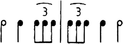
A comparison between the present "reciprocal diminishing returns model" and McAuley's "generalized multiple-look model" is possible if the parameter W of the latter model is established for each of the 25 S/C combinations in which the number of intervals in S increases from 1 to 5, and the number of intervals in C also from 1 to 5. This yields the matrix:
$$ \begin{array}{*{20}{c}} {{{\text{W}}_{{{11}}}}} \hfill & {{{\text{W}}_{{{21}}}}} \hfill & {{{\text{W}}_{{{31}}}}} \hfill & {{{\text{W}}_{{{41}}}}} \hfill & {{{\text{W}}_{{{51}}}}} \hfill \\ {{{\text{W}}_{{{12}}}}} \hfill & {{{\text{W}}_{{{22}}}}} \hfill & {{{\text{W}}_{{{32}}}}} \hfill & {{{\text{W}}_{{{42}}}}} \hfill & {{{\text{W}}_{{{52}}}}} \hfill \\ {{{\text{W}}_{{{13}}}}} \hfill & {{{\text{W}}_{{{23}}}}} \hfill & {{{\text{W}}_{{{33}}}}} \hfill & {{{\text{W}}_{{{43}}}}} \hfill & {{{\text{W}}_{{{53}}}}} \hfill \\ {{{\text{W}}_{{{14}}}}} \hfill & {{{\text{W}}_{{{24}}}}} \hfill & {{{\text{W}}_{{{34}}}}} \hfill & {{{\text{W}}_{{{44}}}}} \hfill & {{{\text{W}}_{{{54}}}}} \hfill \\ {{{\text{W}}_{{{15}}}}} \hfill & {{{\text{W}}_{{{25}}}}} \hfill & {{{\text{W}}_{{{35}}}}} \hfill & {{{\text{W}}_{{{45}}}}} \hfill & {{{\text{W}}_{{{55}}}}} \hfill \\ \end{array} $$in which the first index stands for the number of intervals in S, and the second one for those in C. When W = 1, only the S intervals determine the DL, and when W = 0, only the C intervals determine the DL. If 0 < W < 1, both S and C determine the DL in a certain weight combination (W and 1-W). Analysis of the pattern of weight combinations in the matrix could reveal whether the contributions of S and C to the DL are comparable to the relative proportions of the slopes of the before (S) and after (C) reciprocal functions.

References
Allan, L. G. (1979). The perception of time. Perception & Psychophysics, 26, 340–354.
Baird, J. C., & Noma, E. (1978). Fundamentals of scaling and psychophysics. New York: John Wiley & Sons.
Blaschke, S. (2009). Zeitwahrnemung in isochronen Sequenzen: Ein Vergleich verschiedener Modelle zum Einfluss des Kontextes auf die Wahrnehmungsleistung [Time perception in isochronous sequences: A comparison of different models as regards the contextual influence on perceptual performance]. Unpublished doctoral dissertation, George-August-Universität Göttingen, Germany.
Bolton, T. L. (1894). Rhythm. The American Journal of Psychology, 6, 145–238.
Cornsweet, T. N. (1962). The staircase method in psychophysics. The American Journal of Psychology, 75, 485–491.
Cowan, N. (1984). On short and long auditory stores. Psychological Bulletin, 96, 341–370.
Drake, C., & Botte, M.-C. (1993). Tempo sensitivity in auditory sequences: Evidence for a multiple-look model. Perception & Psychophysics, 54, 277–286.
Fastl, H., & Zwicker, E. (2007). Psychoacoustics: Facts and models. Berlin: Springer Verlag.
Fraisse, P. (1956). Les structures rythmique. Louvain, Belgium: Publications Universitaires de Louvain.
Fraisse, P. (1967). Le seuil différentiel de durée dans une suite régulière d’intervalles. L'Année Psychologique, 1, 43–49.
Friberg, A., & Sundberg, J. (1995). Time discrimination in a monotonic, isochronous sequence. Journal of the Acoustical Society of America, 98, 2524–2531.
Grondin, S. (2001a). Discriminating time intervals presented in sequences marked by visual signals. Perception & Psychophysics, 63, 1214–1228.
Grondin, S. (2001b). From physical time to the first and second moments of psychological time. Psychological Bulletin, 127, 22–44.
Grondin, S. (2010). Timing and time perception: A review of recent behavioral and neuroscience findings and theoretical directions. Attention, Perception, & Psychophysics, 72, 561–582.
Grondin, S., & McAuley, J. D. (2009). Duration discrimination in crossmodal sequences. Perception, 38, 1542–1559.
Grondin, S., Bisson, N., & Gagnon, C. (2011). Sensitivity to time interval changes in speech and tone conditions. Attention, Perception, & Psychophysics, 73, 720–728.
Guttman, N., & Julesz, B. (1963). Lower limits of auditory periodicity analyses. Journal of the Acoustical Society of America, 35, 610.
Halpern, A., & Darwin, C. (1982). Duration discrimination in a series of rhythmic events. Perception & Psychophysics, 31, 86–89.
Hibi, S. (1983). Rhythm perception in repetitive sound sequence. Journal of the Acoustical Society of Japan (E), 4, 83–95.
Hirsch, I. J., Monahan, C. B., Grant, K. W., & Singh, P. G. (1990). Studies in auditory timing: 1. Simple patterns. Perception & Psychophysics, 47, 215–226.
Ivry, R. B., & Hazeltine, R. E. (1995). Perception and production of temporal intervals across a range of durations: Evidence for a common timing mechanism. Journal of Experimental Psychology. Human Perception and Performance, 21, 3–18.
Jones, M. R., & Yee, W. (1997). Sensitivity to time change: The role of context and skill. Journal of Experimental Psychology. Human Perception and Performance, 23, 693–709.
Loveless, N., Levänen, S., Jousmäki, V., Sams, M., & Hari, R. (1996). Temporal integration in auditory sensory memory: Neuromagnetic evidence. Electroencephalography and Clinical Neurophysiology, 100, 220–228.
Lunney, H. W. M. (1974). Time as heard in speech and music. Nature, 249, m592.
Mach, E. (1922). Die Analyse der Empfindungen (Neunte Auflage). Jena: Gustav Fisher Verlag.
Madison, G., & Merker, B. (2002). On the limits of anisochrony in pulse attribution. Psychological Research, 66, 201–207.
Massaro, D. W., & Loftus, G. R. (1996). Sensory and perceptual storage: Data and theory. In E. L. Bjork & R. A. Bjork (Eds.), Memory (Handbook of perception and cognition) (2nd ed., pp. 67–99). San Diego: Academic.
McAuley, J. D., & Kidd, G. R. (1998). Effect of deviations from temporal expectations on tempo discrimination of isochronous tone sequences. Journal of Experimental Psychology. Human Perception and Performance, 24, 1786–1800.
McAuley, J. D., & Miller, N. S. (2007). Picking up the pace: Effects of global temporal context on sensitivity to the tempo of auditory sequences. Perception & Psychophysics, 69, 709–718.
Michon, J. A. (1964). Studies on subjective duration: I. Differential sensitivity in the perception of repeating temporal sequences. Acta Psychologica, 22, 441–450.
Miller, N. S., & McAuley, J. D. (2005). Tempo sensitivity in isochronous tone sequences: The multiple-look model revisited. Perception & Psychophysics, 67, 1150–1160.
Nakajima, Y., ten Hoopen, G., Sasaki, T., Yamamoto, K., Kadota, M., Simons, M., et al. (2004). Time-shrinking: The process of unilateral temporal assimilation. Perception, 33, 1061–1079.
Panissal-Vieu, N., & Drake, C. (1998). Tempo-perception: The multiple-look strategy is limited by a short temporal window. Journal of the Acoustical Society of America, 103, 2849.
Rammsayer, T. H., & Grondin, S. (2000). Psychophysics of human timing. In R. Miller (Ed.), Time and the brain (Conceptual advances in brain research) (pp. 157–167). Reading: Harwood Academic.
Ross, B., Picton, T. W., & Pantev, C. (2002). Temporal integration in the human auditory cortex as represented by the development of the steady-state magnetic field. Hearing Research, 165, 68–84.
Schulze, H.H. (July, 2005). Detectability of uneven rhythms. Paper presented at the 10th Rhythm Perception and Performance Workshop, Bilzen, Belgium.
Siegel, S., & Castellan, N. J., Jr. (1988). Nonparametric statistics (2nd ed.). New York: McGraw-Hill.
Stetson, R. H. (1905). A motor theory of rhythm and discrete succession. Psychological Review, 12, 250–270. and 292-350.
ten Hoopen, G. (February, 1992). Temporal processing of fast auditory patterns. Paper presented at the 2nd International Conference on Music Perception and Cognition, Los Angeles, California.
ten Hoopen, G., Miyauchi, R., & Nakajima, Y. (2008). Time-based illusions in the auditory mode. In S. Grondin (Ed.), Psychology of time (pp. 139–187). Bingley: Emerald Group Publishing Limited.
ten Hoopen, G., Boelaarts, L., Gruisen, A., Apon, I., Donders, K., Mul, N., et al. (1994). The detection of anisochrony in monaural and interaural sound sequences. Perception & Psychophysics, 56, 110–120.
ten Hoopen, G., Hartsuiker, R., Sasaki, T., Nakajima, Y., Tanaka, M., & Tsumura, T. (1995). Perception of auditory isochrony: Time-shrinking and temporal patterns. Perception, 24, 577–593.
Tervaniemi, M., Saarinen, J., Paavileinen, P., Davilona, N., & Näätänen, R. (1994). Temporal integration of auditory information in sensory memory as reflected by the mismatch negativity. Biological Psychology, 38, 157–167.
Winkler, I., Czigler, I., Jaramillo, M., Paavilainen, P., & Näätänen, R. (1998). Temporal constraints of auditory event synthesis: Evidence from ERPs. NeuroReport, 9, 495–499.
Yabe, H., Koyama, S., Kakigi, R., Gunji, A., Tervaniemi, M., & Kaneko, S. (2001). Automatic discriminative sensitivity inside temporal window of sensory memory as a function of time. Brain Research. Cognitive Brain Research, 12, 39–48.
Yee, W., Holleran, S., & Jones, M. R. (1994). Sensitivity to event timing in regular and irregular sequences: Influences of musical skill. Perception & Psychophysics, 56, 461–471.
Author Note
Stéphanie van den Berg is now at the University of Twente, Enschede, The Netherlands. Jiska Memelink is still at Leiden University, Leiden, The Netherlands. Bruno Bocanegra is now at the Erasmus University, Rotterdam, The Netherlands. Roel Boon is now at the Police Academy of The Netherlands, Apeldoorn, The Netherlands. We are very grateful to Edwin van Buuringen for pilot studies and programming. We thank an anonymous reviewer, Devin McAuley, and Simon Grondin for their many helpful comments. We dedicate this study to Carolyn Drake, a great scholar and great lady who unfortunately, but for reasons we respect, left our field. Correspondence concerning this article to Gert ten Hoopen (hoopenten@planet.nl).
Open Access
This article is distributed under the terms of the Creative Commons Attribution Noncommercial License which permits any noncommercial use, distribution, and reproduction in any medium, provided the original author(s) and source are credited.
Author information
Authors and Affiliations
Corresponding author
Rights and permissions
Open Access This is an open access article distributed under the terms of the Creative Commons Attribution Noncommercial License (https://creativecommons.org/licenses/by-nc/2.0), which permits any noncommercial use, distribution, and reproduction in any medium, provided the original author(s) and source are credited.
About this article
Cite this article
Ten Hoopen, G., Van Den Berg, S., Memelink, J. et al. Multiple-look effects on temporal discrimination within sound sequences. Atten Percept Psychophys 73, 2249–2269 (2011). https://doi.org/10.3758/s13414-011-0171-1
Published:
Issue Date:
DOI: https://doi.org/10.3758/s13414-011-0171-1