
Abstract
Nanopores are cost-effective digital platforms, which can rapidly detect and identify biomolecules at the single-molecule level with high accuracy via the changes in ionic currents. Furthermore, nanoscale deoxyribonucleic acid and proteins, as well as viruses and bacteria that are as small as several hundred nanometers and several microns, respectively, can be detected and identified by optimizing the diameters of a nanopore according to the sample molecule. Thus, this review presents an overview of the methods for fabricating nanopores, as well as their electrical properties, followed by an overview of the transport properties of ions and analyte molecules and the methods for electrical signal analysis. Thus, this review addresses the challenges of the practical application of nanopores and the countermeasures for mitigating them, thereby accelerating the construction of digital networks to secure the safety, security, and health of people globally.
Export citation and abstract BibTeX RIS
1. Introduction
Since the discovery of Avogadro's number, the detection and identification of analyte molecules have been largely based on weighting statistics (the statistical averages of ∼1023 molecules have been measured). However, weighting statistics cannot measure the most fundamental physical quantities, such as the number of molecules; counting statistics are employed for detections and identifications based on single-molecule measurements. Thus, the single molecule whose type has been determined can be counted in ones and twos. Counting statistics facilitates a qualitative analysis for detecting and identifying very small amounts of analyte molecules at the single-molecule level. 1–4) This method can be extended to the qualitative analysis of n-type molecules. 1–4) The counting of molecules whose types can be determined ensures the quantitative analysis of the amounts of such molecules in a solution. The counting statistics method can be used to quantitatively determine the existence ratios of molecular species in a solution containing n-types of analyte molecules. Notably, single-molecule-measurement-based qualitative and quantitative analyses will revolutionize biomolecular testing and disease diagnoses.
Nanopore measurement accounts for a typical single-molecule measurement. 5–12) Nanopores can detect and identify particles and biomolecules that pass through them via the changes in the ionic currents flowing through their through-holes with diameters of several nanometers or more [Figs. 1(a) and 1(b)]. Nanopores are classified into two categories, namely, bionanopores 5–12) and solid-state nanopores. 9,13–16) Bionanopores are commercialized next-generation deoxyribonucleic acid (DNA) sequencers that exert a revolutionary impact on medical science. 17–25) There are several review articles on bionanopores. 9,10,12) However, this review focuses on solid-state nanopores. Henceforth, nanopores will be referred to as solid-state nanopores in this paper.
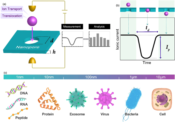
Fig. 1. (Color online) Nanopore digital platform. (a) This digital platform comprises nanopore devices, instrumentation, and data analysis systems. Its practical application requires the development of these two hardware and one software as well as the elucidation of the ion transport and translocation of the analyte molecule in the nanopores. (b) Conceptual diagram of the nanopore sensor principle. An ionic current is obtained when a DC voltage is applied between the electrodes. When the analyte molecule enters the nanopore, the ionic current changes. (c) Biomolecules on a wide range of scales can be detected and identified by generating nanopores with the appropriate diameter for the analyte molecules.
Download figure:
Standard image High-resolution imageNanopores can measure a wide range of biomolecules. 13,26–42) By optimizing the diameter of a solid-state nanopore to the size of the sample molecule, nanoscale DNA and proteins, as well as viruses and bacteria of several hundred nanometers and several micrometers, respectively, can be measured on a single-unit basis [Fig. 1(c)]. Nanopores are digital platforms that detect and identify a wide range of biomolecules of different sizes ranging from the nm to μm scale via the optimization of the nanopore diameter. The development of peptide and protein sequencers using nanopores has recently become a new trend. 43) In addition, clinical specimens have been used to demonstrate a new method for testing for novel coronaviruses. 44)
The nanopore digital platform comprises nanopore devices, instrumentation, and analysis methods [Fig. 1(a)]. The ionic current–time waveforms obtained from this platform facilitate the ion transport in nanopores, as well as the flow dynamics of the analyte particles and molecules. Many researches have contributed to the development of methods for fabricating nanopore devices, 45–47) elucidation of the mechanisms of their electrical properties, 45,48) establishment of the basic concept of flow dynamics, 49–51) and development of analytical methods. 3,4,52) The commercialization of nanopores has been achieved via these comprehensive studies (Nanopore Solutions, Goeppert, and Aipore). Rapid, accurate, inexpensive, and portable methods for conducting biomolecular testing and disease diagnoses using nanopores are currently approaching the practical application stage.
Thus, this review addressed the existing state-of-the-art developments in nanopore fabrication methods, noise reduction in instrumentation, interpretation of measurement data, and analyses of obtained data to reveal significant connections between the relevant results obtained in numerous studies worldwide. Thus, each section will present the challenges of the practical application of specific nanopore-based biomolecular testing and disease diagnoses as well as recommend solutions to the discussed challenges.
2. Nanopore devices
The materials and methods for fabricating nanopores significantly affect the reproducibility and robustness of the ion-current measurements, as well as the mass production and integration of nanopores. The material properties also affect the electrical noise characteristics and flow dynamics of nanopores. Many microfabrication processes have been developed for silicon. Therefore, the consistency of the fabrication process of nanopores through the manufacturing process of silicon semiconductors is a shortcut to the practical application of nanopores. Historically, nanopores have been developed via the fabrication of through-holes in hollow silicon nitride membranes (silicon nitride thin films exhibiting a thickness of ∼50 nm) on a silicon substrate. 9,14,45,47)
2.1. Fabrication method
The foremost nanopores were fabricated in hollow silicon nitride on a silicon substrate employing a focused ion beam (FIB) [Fig. 2(a)]. 13) A secret method for fabricating the nanopores (diameter = 1.8 nm) involved the utilization of a low-stress silicon nitride thin film fabricated via low-pressure chemical vapor deposition. The low-stress property of the thin film ensured the stable fabrication of the through-holes in the membrane. Next, using the intense electron beam of a transmission electron microscope (TEM), nanopores of a few nanometers were fabricated in the hollow silicon dioxide thin film that had been fabricated on the silicon substrate via thermal oxidation [Fig. 2(b)]. 15) The combination of this material with the electron beam of TEM became the standard for the material and fabrication method for nanopores with diameters of a few nanometers.
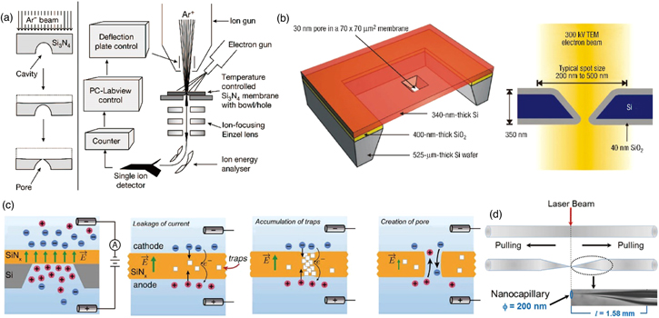
Fig. 2. (Color online) Nanopore fabrication methods. (a) FIB-based fabrication. Here, nanopores with a diameter of 1.8 nm were fabricated on a SiN membrane. Reprinted with permission from Ref. 13. Copyright 2001 Springer Nature. (b) TEM-based fabrication. Here, nanopores with a 2 nm diameter were fabricated on a SiO2 membrane. Reprinted with permission from Ref. 15. Copyright 2003 Springer Nature. (c) CDB-based fabrication. Here, nanopores with a 3 nm diameter were fabricated on a SiN membrane. Reprinted with permission from Ref. 53 (d) Capillary-based fabrication. Here, nanopores with a ∼20 nm diameter were fabricated. Reprinted with permission from Ref. 58. Copyright 2013 American Chemical Society.
Download figure:
Standard image High-resolution imageOwing to their slow production throughput, FIB and TEM do not represent a suitable microfabrication technique for mass-producing nanopores. As a fabrication method with high throughput, electron beam lithography (EBL) has been used to develop nanopores for silicon nitride membranes on silicon substrates. 45–47) The combination of this method with etching and VD can achieve the fabrication of nanopores with diameters of ≥300 nm, although such a combination cannot facilitate the production of nanopores with diameters of a few nanometers. 45–47) Furthermore, as a fabrication method that does not require heavy and expensive equipment, the controlled dielectric breakdown (CDB) method was developed for the fabrication of nanopores via the application of a voltage of 11–17 V between silicon nitride membranes (thickness = 10–30 nm) on a silicon substrate [Fig. 2(c)]. 53–56) The physical breakdown caused by a localized strong electric field facilitates the formation of nanopores with a 2 nm diameter. CDB is a simple process, although the control of the location and number of produced nanopores could be challenging. As a method that does not require microfabrication techniques, a capillary is first formed by heating and pulling a glass pipette, after which nanopores are fabricated in the capillary that is blocked by chemical etching [Fig. 2(d)]. 57–59) This fabrication technique can be used to produce nanopores with diameters of ≥20 nm. Although many nanopore fabrication methods have been developed, nanopores for practical applications are generally fabricated via EBL, which is semiconductor technology. By con-chambering mass productivity, high reproducibility, and high yield, nanopores with diameters of 300 nm could be developed via EBL for future practical applications. Practical methods for fabricating nanopores with diameters of <300 nm have not yet been established, and this represents the biggest barrier to the practical applications of nanopores.
2.2. Materials
Following their development history, nanopores have been fabricated on silicon nitride membranes, although SiO2, 60–62) HfO2, 63,64) Al2O3, 63,65) ZnO, 66) and TiO2 67) have also been used as alternatives. The development of nanopores involves two approaches: decreasing the diameter of the nanopore and decreasing its thickness. The spatial resolution of the ionic current–time waveforms, which is obtained via nanopore measurements, could improve with the decreasing nanopore thickness (the ideal thickness of a nanopore is one atomic layer). Two-dimensional materials, such as graphene sheets, 16,26,27,68–76) MoS2, 28,77–79) WS2, 80) and h-BN, 81–83) have been utilized to fabricate nanopores in membrane structures comprising several atomic layers. The nanopores were fabricated by focusing ion or electron beams from FIB or TEM, respectively, on two-dimensional (2D) materials that had been fabricated on support substrates, such as silicon substrates. Nanopores (diameter = 5 nm), which were fabricated on several layers of MoS2, were successfully used to identify single DNA base molecules. 28) Although the high spatial resolutions of thin membranes have been demonstrated, the development of fabrication methods that enables the mass production of 2D material-based nanopores with high reproducibility and yield accounts for a major barrier to their practical application.
Thinner films are essential for nanopore-based measurements for identifying biomolecules on a molecule-by-molecule basis with high precision. 49) Thinner films pose a new challenge to researchers because thinner nanopores correspond to the generation of stronger electric fields within the nanopore. 49) This relatively stronger electric field allows biomolecules to pass through the nanopores much faster during electrophoresis. To achieve a high spatial resolution, the measurement must be rapidly conducted or the translocation of a single molecule decelerated. Studies on faster measurements are reported in the next section (Sect. 3), and those of slower single-molecule velocities are presented in Sect. 4. The two consecutive sections reveal that the methods for fast measurement and slow translocation are inextricably linked to the device materials and fabrication methods.
3. Current measurement methods
The origin of the current obtained during nanopore measurement, where a DC voltage is applied, is ionic and electronic transport. The characteristic electrical properties in nanopore measurements, represented by rectangularity, are mainly due to ionic conductivity. Conversely, the characteristic electrical noise is mainly due to the flicker noise,  thermal noise,
  insulator noise,
  and capacitive noise,
  which originate from electron transport [Fig. 3(a)].
45,48,84) These four types of noise account for the noise in nanopore measurements; the frequency bands in which the four types of noise dominate are fixed. The total noise,
which originate from electron transport [Fig. 3(a)].
45,48,84) These four types of noise account for the noise in nanopore measurements; the frequency bands in which the four types of noise dominate are fixed. The total noise,  of the measurement system is given by Eq. (1):
In addition, if the power spectral densities (PSD) corresponding to each noise are 

 and
and  the PSD,
  of the measurement system will be presented by Eq. (2):

The PSD and the current noise exhibit the following relationship:


Fig. 3 (Color online) Electrical noise in nanopores. (a) Frequency dependence of noise. The noise spectral density, S(f), was fitted by S(f) = A/f + B + C f + D f2. The bandwidth of flicker noise is <100 Hz. The bandwidth of the thermal noise is between 100 Hz and 2 kHz. The bandwidth of the dielectric noise is 1–10 kHz. The bandwidth of the capacitive noise is >10 kHz. Reprinted with permission from Ref. 84. Copyright 2016 American Chemical Society. (b) Noise currents in the nanopores (diameter = 20 nm) that were fabricated on Si3N4 membranes on various substrates. Reprinted with permission from Ref. 97. Copyright 2014 Springer Nature. (c) Frequency dependence of PSDs of the nanopores (diameter = 20 nm) that were fabricated using SiN membranes and Si thin films on Si substrates and quartz, respectively. Reprinted with permission from Ref. 97. Copyright 2014 Springer Nature. (d) Device structures comprising nanopores with diameters of less than 3.5–4.9 nm were fabricated using SiN membranes on SOI. Reprinted with permission from Ref. 61. Copyright 2012 Springer Nature. (e) Optical photograph of a preamplifier, which was fabricated in a complementary metal–oxide semiconductor (CMOS), and the schematic diagram of a current amplifier. Reprinted with permission from Ref. 61. Copyright 2012 Springer Nature. (f) Frequency dependence of the noise spectral density of the CMOS-integrated nanopore platform with a 4.9 nm diameter. Axopatch shows the standard instrumentation employed in nanopore metrology (Axopatch 200B). Reprinted with permission from Ref. 61. Copyright 2012 Springer Nature.
Download figure:
Standard image High-resolution image3.1. Flicker noise
The flicker noise in the low-frequency band is also referred to as the 1/f noise. The impurity and trapped levels account for the source of flicker noise in semiconductors. Flicker noise is obtained using the following equation as Hooge's relation: 85)

where α and β denote the Hooge parameters that are associated with the membrane material of the nanopore (fitting parameters with values close to 1). Nc, I, and f denote the number of charge carriers in the nanopore, the ionic current obtained by the measurement, and the frequency, respectively. The flicker noise in the nanopores is caused by the vibration of the membrane, 82,86,87) the charge in the nanopores, 88) and the adhesion of the impurities and nanobubbles on the surface of the nanopore. 89) The membranes that are deposited on silicon substrates mechanically vibrate in the presence of thinner films and larger areas. Graphene membranes comprising several layers exhibit two orders of magnitude-greater noise than SiN membranes with a thickness of several ten nanometers. 26,90) Flicker noise is reduced by decreasing the area. Impurity removal and surface modification are effective strategies for reducing noise in nanopores, as in semiconductors. Furthermore, cleaning the SiN membrane with a piranha solution (30% H2O2:H2SO4 = 1:3) could reduce the flicker noise by a factor of 100 compared with no cleaning. 91)
3.2. Thermal noise
When the temperature and nanopore resistance are T and RPore, the PSD of the thermal noise can be expressed as follows: 92,93)

where k is Boltzmann's constant. Thermal noise, which is caused by the irregular movement of electrons through a resistive element in response to heat, exists in all resistive elements. Thermal noise can never be smaller than Eq. (5), even if the other three noises can be significantly reduced. Using Eqs. (3) and (5), the thermal noise voltage can be expressed as follows:

At room temperature (T = 300 K), RPore = 100 MΩ and f = 100 Hz, amounting to 13 μV. At 250 kHz, which is the typical measurement bandwidth for nanopores, this value will be 643 μV. Because the resistance of a nanopore cannot be reduced, its thermal noise can only be reduced by lowering the temperature or measurement bandwidth. The AxoPatch 200B utilizes a Peltier effect to lower the temperature.
3.3. Dielectric noise
Given that the capacitance and dielectric loss of the nanopore device are CPore and DPore, respectively, the PSD of the dielectric noise will be represented by Eq (7): 94)

where CPore can be controlled by the device structure and materials. By coating the membrane with a dielectric material, such as polyimide or silicone, CPore could be reduced, thereby reducing the noise by one to two orders of magnitude. 91,95,96) In addition, the noise was reduced by a factor of 10 [Figs. 3(b) and 3(c)] by changing from a silicon substrate to an insulating one, such as glass. 97) The structure combining these two methods reduced the capacitance of the device comprising a SiN membrane on a silicon substrate from 300 to 6 pF. 61) In this structure, the SiN membrane is deposited on a silicon-on-insulator (SOI) substrate comprising a SiO2 thin film on the silicon substrate, and the SiN membrane is coated with silicone as the insulator [Fig. 3(d)]. 61) The situation in which both chambers of the SiN membrane are filled with a solution containing ions is equivalent to that of the parallel-plate model in which the insulator is sandwiched between conductors. In this model, reduction of the area of the SiN membrane in contact with the solution reduces CPore. The reduction of the membrane area is equivalent to the method for reducing flicker noise due to membrane vibration. Thus far, the reviewed noise-reduction methods have availed design guidelines for low-noise nanopore devices. The design guidelines comprise fabricating a small-area membrane on an insulating or SOI substrate, coating the membrane with an insulator, and cleaning the nanopore device with a piranha solution.
3.4. Capacitive noise
Given that the capacitances of the nanopore device, current amplifier, and wiring are CPore, CAmp, and CWire, respectively, the PSD of the capacitive noise can be represented by the following equation: 98)

where vn denotes the noise density of the input voltage. The reduction of noise by reducing CPore is common with the methods for reducing insulation noise. Therefore, it is consistent with the design guidelines of noise-reduction devices, which have been discussed (Sect. 3.3). When the wiring is parallel along the same plane, CWire will be proportional and inversely proportional to the height of and distance between the wiring, respectively. CWire can be minimized by designing the interconnections according to this rule. The reduction of capacitive noise mainly depends on minimizing CAmp.
Presently, 100 kHz low-pass filters are employed as standards owing to the high electrical noise in the high-frequency band. To identify the high-accuracy molecules passing through nanopores at speeds of >100 kHz, it is important to reduce the electrical noise in the high-frequency band. The ionic currents obtained from the nanopore measurements range from a few pA to several 10 nA. To measure ionic currents, the input current is amplified and output as a voltage (transimpedance amplifiers (TIA) are utilized in most cases). Ideally, TIA must be able to measure currents with high sensitivities over a wide frequency band, and the noise gain (NG) around the cut-off frequencies, fc, and fc of TIA is determined using the following equation, where Rf and Cf denote the feedback resistance and feedback capacitance of the amplifier, respectively:


where Rf is the current amplification factor. At Rf = 100 MΩ, an ionic current of 1 pA is amplified to 108 Ω × 10−12 A = 0.1 mV. To reduce the amplifier noise, CPore or Cf can be reduced or increased, respectively. However, the cut-off frequency can be reduced by increasing Cf, thereby inhibiting fast measurements. In practice, this corresponds to reducing CPore. By integrating TIA into an integrated circuit comprising a small feedback resistor fabricated from a metal–oxide–semiconductor field-effect transistor and a silicone-coated SiN membrane fabricated on an SOI substrate, a bandwidth performance of 1 MHz was achieved at Cf = 0.15 pF [Figs. 3(e) and 3(f)]. 61) Moreover, the signal-to-noise ratio (SNR) was >10. The advantage of using TIAs as integrated circuits is the noise reduction via the minimization of parasitic capacitance due to the shortest distance between TIA and the nanopore. Another advantage involves the parallel measurement facilitated by integrating many nanopore devices on a single chip. Thus, the most effective method for using nanopores for the measurement of ionic currents at a high speed and with low noise is to deposit a small-area membrane on an insulating or SOI substrate and to cover the membrane with an insulator.
4. Flow dynamics
The ionic current–time waveforms obtained from the nanopores were observed from two perspectives, namely, ion transport and the translocation of the analyte molecule. Furthermore, the magnitude of the base current, as well as the current–voltage characteristic of the buffer solution-filled nanopores, was observed to determine whether the measurement system worked correctly. Ion transport is employed to confirm the correct operation of the measurement system. When measuring the buffer solutions of sample molecules, the signal frequency and ionic current–time waveform of the analyte molecules were observed. The signal frequency determines the throughput of the test/diagnostic time, whereas the ionic current–time waveform determines the accuracy of detecting and identifying the analyte molecules. The translocation of analyte molecules determines the testing and diagnostic performances.
When an Ag/AgCl electrode (as the electrode) and a solution containing Cl− are utilized, the ionic current obtained is due to the electrochemical reactions occurring at the electrode interface. The ions, which are present around the nanopores, do not directly convey the information associated with the translocation of the analyte molecules to the electrodes through the nanopores. This is evident because most of the voltages applied between the electrodes are applied between the membranes. Nanopore measurements reveal the dynamics of the ions, and the flow dynamics of charged analyte molecules flowing through the nanopores facilitate detection and diagnosis. The dynamics of the ions, as well as the flow dynamics of the analyte molecules, are inextricably linked. Ion transport consists of ion dynamics. The translocation of an analyte molecule comprises the ion and flow dynamics of the analyte molecules.
4.1. Ion transport
The transport of ions in nanopores is evaluated using the simplest model. Therein, the ionic current in V/RPore is evaluated as the base current when the applied voltage is V. The resistance is given by Eq. (11) if the ionic resistivity of the buffer solution is ρ: 99)

When using a typical buffer, 1X PBS (ρ = 1.6 Sm−1), and nanopores (diameter and thickness = 300 and 50 nm, respectively), the value of RPore would be 2.5 MΩ. Notably, this model does not apply to all nanopores; for example, Eq. (11) applies to cylinder-shaped nanopores. The resistance of a nanopore depends on its structure. 51,100–105) In practice, many nanopores exhibit a truncated cone shape. The surface charge of the nanopore is also the main reason why Eq. (11) cannot be applied. 51) The surface charge of the nanopore generates an electro-osmotic flow along the wall of the nanopore; this flow affects the ionic current–voltage curve. The ionic current–voltage curve is an indicator of the strength of the surface charge. The detailed mechanism of ionic current–voltage curves indicating rectification is reported in other reviews. 50,51) In this review, the mechanisms that must be elucidated to add the desired functionality to nanopore measurement systems are presented.
The forces acting on ion transport depend on the distance between the interacting substances. 106) For example, hydration and steric hindrance act predominantly at an interaction distance <2 nm; the van der Waals forces, interaction distance <50 nm; and electrostatic interaction, interaction distance <100 nm. A typical electrostatic interaction involves that between the charges on the nanopore wall and the ions in the solution. The models of ion transport can be broadly divided into two categories depending on the diameter of the nanopore. 50) When the diameter is >5 nm, ion transport is described by the continuum model, and when the diameters are >5 nm, the ion transport is described by molecular dynamics. At present, molecular dynamics is challenging to model, and a timescale is used to simulate the amorphous membranes to reproduce experimental results. 50)
The continuum model avails a picture of the dynamics of ion transport to the experimenter. The walls of the SiN membrane are charged to −44 mC m−2, and the experimental zeta potential of the Si3N4 surface ranges from −18 to −26 mV. 107,108) The walls of the SiN membrane are charged by electrostatic cations that accumulate on the SiN membrane wall via electrostatic interaction (cations accumulate on the SiN membrane wall via electrostatic interaction). This accumulation layer is known as the stern layer. The bulk ion concentration (nBulk) is reached above the Debye length (λD) from the stern layer. Given that the dielectric constant of the solution, electric elementary mass, and valency of the ions are ε, e, and Z, respectively, λD would be represented by Eq. (12):

At nBulk = 100 mM for the monovalent ions, λBulk is 1 nm. A positive voltage is applied to the cis chamber, including Region I, whereas the trans chamber, including Region II, is grounded [Fig. 4(a)]. 109) The cations in the solution and those accumulated on the nanopore wall would migrate from the cis to trans chambers. Thus, the ion concentrations of the trans and cis chambers would increase and decrease, respectively. This difference between the ion concentrations induces the diffusion of ions from the trans to cis chambers. The diffusion of ions suppresses and enhances the electrophoretic cation and anion fluxes, respectively. When a positive voltage is applied to the trans chamber while grounding the cis chamber, the cation and anion fluxes are also suppressed and enhanced, respectively. However, the cation flux, following the application of a positive voltage to the cis chamber, is different from that, following the grounding of the chamber. Similarly, the anion flux depends on voltage polarity. This flux difference generates a rectification property. The rectification factor (RF) is greater for nanopores exhibiting smaller diameters [Fig. 4(b)]. 109) Particularly, when the diameter is <50 nm, the rectification ratio rapidly increases. RF also increases with the bias voltage (the surface charge), thereby increasing the thickness of the wall of the nanopore surface [Figs. 4(c)–4(e)]. 109) Furthermore, RF increases with the decreasing concentration of the buffer solution [Fig. 4(f)]. 109) RF determines the degree of nonlinearity of the ionic current–voltage curve. The degree of nonlinearity obtained from the measurement facilitates the optimization of the measurement protocol. Increasing the ion concentrations of the buffer reduces the influence of the surface charges on the nanopore surface wall. High ion concentrations generate large ion currents, thus increasing SNR. Notably, high ion concentrations can agglomerate analyte molecules with the surface charge.
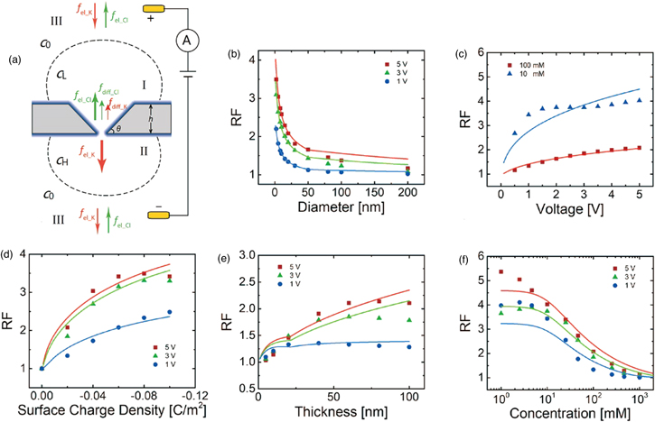
Fig. 4. (Color online) Ion transport in nanopores. (a) Distributions of the ion flux and concentration in nanopores exhibiting negatively charged surfaces. The solution contains KCl. fel_K and fel_Cl denote the ion fluxes of K+ and Cl− via electrophoresis, respectively. fdiff_K and fdiff_Cl denote the ion fluxes of K+ and Cl− due to the concentration gradient-driven diffusions, respectively. CL and CH denote low and high concentrations, respectively. C0 indicates the bulk ion concentration. In Region III, the ion fluxes of K+ and Cl− were almost balanced. In Regions I and II, the balance between fel_K and fel_Cl was broken by the ion selectivity of the nanopores. Dependences of the rectification ratio (RF) on the (b) diameter, (c) voltage, (d) surface charge, (e) nanopore thickness, and (f) concentration. Reprinted with permission from Ref. 109. Copyright 2019 American Chemical Society.
Download figure:
Standard image High-resolution image4.2. Translocation of the analyte molecules
The surface charges on the nanopore walls, as well as the structure and surface charges of the analyte molecule, could complicate the translocation dynamics of the analyte molecule through the nanopores [Figs. 5(a) and 5(b)]. 110,111) Moreover, the translocation dynamics of the analyte molecule change the ion transport to obtain an altered ion transport in the measurement. Theoretical studies coupling the translocation dynamics of an analyte molecule with ion transport are less common than those on ion transport. The theoretical studies use the molecular dynamics methods for nanopores exhibiting diameters of a few nanometers, 112–114) as well as multiphysics simulations for nanopores exhibiting diameters of more than a few 10 nm. 115–120) Multiphysics simulations combine three physical models that describe the ionic dynamics of the nanopore. The interface between the nanopore and liquid is described by the Poisson–Boltzmann equation. Ion transport via diffusion, an electric field, and advection is described by the Nernst–Planck equation. The Navier–Stokes equation also describes the motion of liquids due to the pressure and viscosity applied to the solution. Multiphysics simulations incorporating the time evolution of an analyte molecule passing through nanopores are challenging. It represents an intrinsic challenge for basic science to connect the models that treat the interactions between the matter, nanopores, water, and ions passing through nanopores on a molecular basis using models that treat them as a continuum. For practical purposes, it is paramount to obtain high signal frequencies. Here, we focused on the capture rate of analyte molecules to demonstrate the transport mechanism of analyte molecules.

Fig. 5. (Color online) Translocation of the analyte molecules. (a) Schematic diagram of the translocation mechanism of the analyte molecules in the nanopores. In Region I, the translocation proceeds when the kinetic energy of the analyte molecule crosses an energy barrier through the nanopore structure. In Region III, the kinetic energy of the analyte molecule competes with the diffusion motion. The boundary between Regions I and III is expressed by the capture radius, r*. Reprinted with permission from Ref. 110. Copyright 2010 Springer Nature. (b) Dynamics of the negatively charged analyte molecules that are translocated through the nanopores exhibiting a negative surface charge. The cations are accumulated on the nanopore surface wall. The movement of the cations generats an electro-osmotic flow. vEP denotes the velocity of the analyte molecule via electrophoresis. vEO indicates the velocity of the analyte molecule via the electro-osmotic flow. The dotted lines on the analyte molecule (particle) and the surface of the nanopore wall indicate the stern layer. vEP and vEO are in the cis and trans chamber orientations, respectively, when a positive voltage was applied to the cis chamber. When a negative voltage was applied to the cis chamber, vEP and vEO were in the trans and cis chamber orientations, respectively. The magnitudes of vEP and vEO determine the transport dynamics of the analyte molecules. Reprinted with permission from Ref. 111. Copyright 2012 American Chemical Society.
Download figure:
Standard image High-resolution imageAssuming that the analyte molecule passing through the nanopore, as well as the surface charge on the nanopore wall, are both negative [Fig. 5(b)], 111) a positive voltage would be applied to the cis chamber, whereas the trans chamber would be grounded. The analyte molecule would be forced to move from the trans to cis chambers via electrophoresis. The electro-osmotic flow acts from the cis chamber to the trans one. The translocation of the analyte molecule from the cis to trans chambers subjects it to a drag force from the liquid from the trans chamber to the cis one. When the electro-osmotic flow is stronger than the electrophoretic force, the analyte molecule passes through the nanopore. Thus, the greater the surface charge of the surface of the nanopore wall, the stronger the electro-osmotic flow, and the lower the ion concentration of the solution, the longer the distance that the electro-osmotic flow would act from the nanopore wall. The magnitude of the surface charge and ion concentration can control the translocation speed of the analyte molecule.
The capture rate, which is crucial to actual measurements, can be classified into two processes [Fig. 5(a)]. Competition exists between the kinetic energy due to the Brownian motion of the analyte molecule and motion toward the nanopore due to the electric field. The radius of the boundary at which this competition occurs, r*, is represented by the following equation, where D and μ denote the diffusions constant and mobility of the analyte molecules, respectively: 110,120)

where ΔV denotes the voltage applied to the nanopore. From the classical Smoluchowski result, the capture rate, RDiff, is represented by Eq. (14): 110,120)

where c denotes the concentration of the analyte molecules. This is the capture rate from Region III, which was captured within Regions I and II [Fig. 5(a)]. The capture rate, R'Diff, con-chambering the electro-osmotic flow, is represented by the following equation, where ζPore and ζA denote the zeta potentials of the wall of the nanopore surface and surface of the analyte molecules, respectively: 111)

The analytical equation, Eq. (15), does not reproduce the experimental results of the silica nanoparticles exhibiting diameters of 50 and 100 nm measured at nanopores exhibiting diameters of 215 nm. 111) This could be due to a poor approximation or estimation of the zeta potential.
The analyte molecules entering Regions I and II approach the nanopores via electrophoretic forces [Fig. 5(a)]. The translocation of the analyte molecules occurs when their kinetic energy exceeds the potential barrier formed by the nanopore space. The capture rate, RP , of the analyte molecule captured in the nanopore is expressed by the following equation if the effective surface charge of the analyte molecule is Q, whereas the potential barrier is U: 110,120,121)

R0 is expressed by Eq. (17) if a double-stranded DNA (dsDNA) is approximated by a cylinder: 115,120)

where VDNA denotes the local DNA velocity in the cis chamber and is proportional to ΔV. Equations (14)–(17) demonstrate that the capture rate increases with the increasing concentration of the sample molecules, applied voltage, nanopore diameter, and surface charge.
Thus far, the discussion has demonstrated that the ionic current–time waveform can avail little information: the analyte molecules passing through the nanopores are detected and identified using the ionic current–time waveform. Real samples, such as clinical specimens, generally contain impurities. The ionic current–time waveform of the mixture of analyte molecules and impurities must be identified to ensure the practicality of the system for measuring such nanopores. Ionic current–time waveforms are obtained via the simulations of time evolution, which are computationally expensive. The translocation of a filamentous virus exhibiting a diameter of 6.6 nm in a nanopore exhibiting a diameter of 26 nm was simulated by the coarse-grained Langevin dynamics. 37) This model neglects the hydrodynamics and water molecules. The same molecular dynamics simulations were performed to measure tobacco mosaic viruses (length/width = 300/18 nm) using nanopores (diameter = 20–50 nm). 40) The simulations offered information on the structure of the molecules passing through the nanopores, as well as the entry motion of the virus into the nanopores. However, molecular dynamics simulations cannot reproduce the experimentally obtained translocation times of the ms order. Thus, the experimentally obtained ionic current–time waveforms have not been simulated.
Multiphysics simulations, which are generally continuum models, are also computationally expensive for the simulations of time evolution. Therein, the analyte molecule is fixed at a single point in space, and the ionic current is obtained via the multiphysics simulation of the steady state at that position. 39,41,122,123) The fixed position is shifted, after which the ionic current at each fixed point is calculated. Using this scheme, the ionic current–time waveform, which is obtained as the analyte molecule passes through the nanopore, is simulated. These simulations reproduced the experimental results of the measurements of polystyrene nanoparticles (diameter = 780 nm) and Streptococcus salivarius (diameter = 800 nm) in nanopores with a 1.2 μm diameter. 41) The ionic current–time waveforms obtained by measuring influenza viruses (diameter = 110 nm) in nanopores exhibiting diameters of 300 nm were also reproduced. 39) It has been demonstrated that the ionic current–time waveform depends on the surface charge, structure, and volume of the analyte molecules. Presently, COMSOL® enables powerful multiphysics simulations. Time-evolving simulations are crucial to the elucidation and engineering of the translocation dynamics of the analyte molecules.
4.3. Methods for reducing translocation speeds
High signal frequency due to high bias voltages increases the throughputs of nanopore-based testing and diagnostics. High bias voltages accelerate the translocation rate of the analyte molecules. As outlined in Sect. 3, the measurement speeds of currents at the pA level are limited by a few MHz. The application of high bias voltages, high signal frequencies, and low translocation rates would be optimal for testing and diagnostics. As outlined in Sect. 4.2, even simulation cannot describe the translocation of the analyte molecules. Thus, the duration of the ionic current–time waveform is used as an indicator to assess the translocation rate. The typical translocation rates of dsDNA in a SiN membrane through nanopores with diameters of a few nanometers are 1–10 ms at an applied voltage, ∣VBias∣, of ∼100 mV. 49)
There are two main methods for reducing the translocation speed: passive and active controls. 124) In the passive control, the viscosity of the solution is controlled. Glycerol was added to the solution to make it highly viscous for the measurement of dsDNA in nanopores exhibiting a diameter of 4–8 nm [Fig. 6(a)]. 29) The translocation speed was five times lower at ∣VBias∣ = 120 mV. The method for controlling the viscosity of a solution was also demonstrated using MoS2 nanopores (diameter = 2.8 nm) with an ionic liquid (IL, BmimPF6) and 2 M KCl in the cis and trans chambers [Fig. 6(b)]. 28) The translocation speed of dsDNA was approximately 100-fold slower. A method for distinguishing ion concentrations in the cis and trans chambers was also developed [Fig. 6(c)]. 110) The KCl concentrations of the cis and trans chambers were 0.2 and 1 M, respectively. The translocation speed of dsDNA was 3.5 times slower when evaluated using nanopores with a diameter of 3.5 nm, at ∣VBias∣ = 300 mV. The capture rate increased by a factor of 30. A method, which involved changing the type and concentration of ions, was developed to increase the shielding effect of ions and reduce the effective charge of DNA [Fig. 6(d)]. 125) The translocation speed of dsDNA through nanopores exhibiting diameters of 15–20 nm in 1 M LiCL was five times lower than that in 1 M KCl at ∣VBias∣ = 120 mV. The capture frequency was reduced to 25%. The chemical modification of the nanopore surface can be used to reduce the translocation speed via the intermolecular interactions between the analyte and modified molecules [Fig. 6(e)]. 126) The surfaces of SiN nanopores with diameters of 16–50 nm were modified with lipid bilayers. The translocation speed of a protein (streptavidin) was reduced to several folds at ∣VBias∣ = 100 mV. Gold-coated SiN nanopore surfaces with a diameter of 300 nm were modified with peptides for the identification of influenza viruses [Fig. 6(f)]. 38) Compared with unmodified SiN, the viral translocation speed was approximately 10-times lower at ∣VBias∣ of 150 mV. A method for reducing the translocation speed of the analyte molecule via the temperature difference between the cis and trans chambers has been theoretically proposed. 117)

Fig. 6. (Color online) Methods for reducing the translocation speed of the analyte molecules. (a) Method controlled by viscosity via the addition of glycerol to the buffer. Viscosity dependence of the changes in the current and translocation times when measuring dsDNA. ■ and ▲ denote the changes in the current and transport times, respectively. Reprinted with permission from Ref. 29. Copyright 2005 American Chemical Society. (b) Method controlled by viscosity via the additions of IL and KCl to the cis and trans chambers, respectively. The blue and orange colors indicate the changes in the current and translocation times using the aqueous solution and IL, respectively, in the measurement of dsDNA. Reprinted with permission from Ref. 28. Copyright 2015 Springer Nature. (c) Method controlled by the ion concentrations of the cis and trans chambers. Here, 400- and 2000-bp DNAs were measured. Ccis dependence of the translocation time (tT). The vertical axis was normalized by Ccis = 1 M. Reprinted with permission from Ref. 110. Copyright 2010 Springer Nature. (d) Method controlled by the ionic species. Histograms of the translocation times at each salt concentration at 1 M. dsDNA were measured. Reprinted with permission from Ref. 125. Copyright 2012 American Chemical Society. (e) Chemical modification of the nanopore surfaces to control the fluidity within the nanopore. Histograms of the translocation times at low and intermediate viscosities (Streptavidin was measured). Reprinted with permission from Ref. 126. Copyright 2012 Springer Nature. (f) Method controlled by the molecular interactions between the surface-modified molecule of the nanopore and the influenza virus A(H1N1). Dependence of translocation time on the modified molecule. P1, P2, and P3 denote the peptide species to be chemically modified. Mode1 and Mode2 indicate the different translocation events. Reprinted with permission from Ref. 38. Copyright 2018 American Chemical Society. (g) Method controlled by the gate voltage. Gate-voltage dependence of the translocation time (dsDNA was measured). Reprinted with permission from Ref. 127. Copyright 2012 American Institute of Physics. (h) Method controlled by the pressure applied to the cis chamber. Histograms of the translocation times at pressurized (blue) and ambient pressure (red) (dsDNA was measured). Reprinted with permission from Ref. 128. Copyright 2013 American Chemical Society. (i) Method for controlling the nanoparticles that were bound to the analyte molecules using optical tweezers. Changes in the current, following the application of mechanical forces (dsDNA was measured). Reprinted with permission from Ref. 129. Copyright 2006 Springer Nature.
Download figure:
Standard image High-resolution imageRegarding the active controls, three methods have been developed. One uses a gate voltage to control the surface charge of the wall of the nanopore surface. Using nanopores (diameter = 20 nm) and dsDNA, a gate voltage of 0.6 V reduced the translocation speed by a factor of 20 at ∣VBias∣ = 150 mV [Fig. 6(g)]. 127) Another method, which involves the application of hydropressure to the cis chamber, was developed [Fig. 6(h)]. 128) By applying hydropressure of 2.44 atm, a dsDNA was translocated at an eight-times lower rate through nanopores exhibiting a diameter of 10 nm (∣VBias∣ was 90 mV, and the capture rate was reduced by a factor of five. Furthermore, a method in which nanoparticles that were bound to one end of the dsDNA were employed to mechanically pull the DNA by light or magnetism was developed [Fig. 6(i)]. 129) Using nanopores (diameter = 6–15 nm) and dsDNA, this technique was demonstrated at ∣VBias∣ = 30 mV. The elucidation of the correlation between the translocation speed and capture rate of the analyte molecules for the passive and active controls is a crucial issue for the future.
A high hurdle, namely, the development of rapid current-measurement techniques, has increased the research on reducing the translocation speed of the analyte molecule. Rapid current-measurement techniques have been developed (Sect. 3). Section 3 elucidated the electrical noise of nanopores well and recommended nanopore structures that can deliver noise reduction. Furthermore, control methods were developed to reduce the translocation speed of the analyte molecules. Thus, an ideal development environment for the detection of analyte molecules with high translocation speed, as well as for controlling the speed if necessary, has been revealed.
5. Methods for analyzing ionic current–time waveforms
The analytical methods for achieving the practical application of nanopore-based testing and diagnostics can be classified into qualitative and quantitative analyses. Qualitative analysis can determine the presence of a new coronavirus type. It can also determine the presence of Influenza A or B in a solution. Practical qualitative analysis requires multiplex analysis, which can simultaneously detect and identify several types of analyte molecules via a single measurement. Quantitative analysis can determine the viral load (the amount of the newly detected coronavirus). Quantitative testing and diagnostics account for a much larger market than qualitative testing and diagnostics. The major hindrance to the practicality of nanopores is the development of multiparameter qualitative and quantitative analysis methods. The ionic current–time waveforms obtained from nanopore measurements are characterized by a low SNR, base current fluctuations, multisteps, and similarity of the different analyte molecules. 3,4,52) The methods for processing waveform data have been developed to address these four features (low SNR, base current fluctuations, multisteps, and similarity of the different analyte molecules). These methods involve denoising, waveform extraction, feature extraction, and identification, respectively. The respective principles of waveform data-processing methods are reported in recent reviews. 3,4,52)
5.1. Denoising methods
The strategies for denoising the hardware of the measurement system, including the devices, are derived from the results outlined in Sects. 2 and 3. SNR could be significantly improved by denoising the hardware. Thus, this section outlines the denoising software that has been developed so far.
In nanopore measurements, a typical denoising method involves the use of a low-pass filter at 100 kHz. Low-pass filters can extract relevant data at high frequencies. Kalman 130) and wavelet 131,132) filters have also been developed to overcome this challenge. These filters can separate still the waveforms obtained from the analyte molecule and noise even in frequency bands where they overlap.
5.2. Extraction methods for ionic current–time waveforms
The ionic current–time waveforms obtained via nanopore measurements are characterized by low SNR, base current fluctuations, and multisteps.
The only requirement for detecting and identifying biomolecules is a waveform that corresponds to the translocation of the analyte molecule; however, it can only measure ion transport. Ion transport contains information on the translocation of the analyte molecule and the change in the ion transport between an electrode pair. The ionic current obtained from the measurement proceeds from the electrochemical reactions at the electrode–liquid interface. Therefore, an Ag/AgCl electrode with an extremely small area and low thickness or the oxidation of that electrode could fluctuate the base current. If the nanopores are clogged with the material, this can also fluctuate the base current. In many cases, multiple peak currents or plateaus were observed in a single ionic current–time waveform. 3,4,52) These multistep waveforms exhibit the translocation properties of the analyte molecule. Thus, multistep analysis methods are crucial. The challenge involves the determination of the beginning and end times of the waveforms. A particular challenge, which was resolved by developing the ADEPT, 133) CUSUM, 134,135) and MOSAIC 136) algorithms, involved the detection of waveforms with short current durations.
ADEPT is a physical model-based algorithm that recovers spike waveforms that are unaffected by distortions due to bandwidth limitations of the data measurement rate of the instrument. 133) This algorithm detects waveforms with short current durations. CUSUM is an abrupt change-detection algorithm that employs the cumulative deviation between the true ionic current–time waveform and the predicted waveform as an indicator of the change in the current level. 134,135) This algorithm facilitates the easy identification of different levels in each event. The CUSUM algorithm can detect waveforms with long current durations. MOSAIC is an integrated algorithm that combines ADEPT and CUSUM+. 136) This algorithm uses a hidden Markov model to facilitate the multistep characterization and detection of waveforms that had been hidden by noise.
5.3. Feature extraction
ADEPT, CUSUM, and MOSAIC perform features and waveform extractions. The features extracted by these nonmachine learning algorithms include the peak current, current duration, and event frequency. The features employed by machine learning are generated by the analyst. The symmetry, kurtosis, and area of the ionic current–time waveform are used as features. 3,38,39,41,42,137) Furthermore, a vector dividing the ionic current–time waveform into n equal parts along the time direction is employed as a feature. 44) Because they are generated by hand by the analyst, it is sometimes possible to physically interpret the features. At present, the Tsfresh package 138) can be used to automatically generate thousands of features from time-series data, such as the ionic current–time waveforms. In machine learning, these features are analyst-dependent. Deep learning is employed to remove the analyst dependency and automatically generate features. The physical interpretation of the features employed in deep learning is impossible.
5.4. Identification of analyte molecules
Typical features, such as the peak current (Ip) and current duration (td), have been employed to identify analyte molecules. Before the introduction of the machine and deep learning, the identification of biomolecules was almost exclusively discussed using the histograms of both features. In a recent representative example, four nucleotides were identified using the nanopore of MoS2 (diameter = 2.8 nm, Fig. 7(a). 28) Four oligonucleotides consisting of 30 base molecules were also identified using a nanopore with a diameter of 1.5 nm. During this single-molecule identification, a technique was employed to reduce the translocation speed of the analyte molecule by introducing IL to the cis chamber. In the measurements employing nanopores without controlling the translocation speed of the analyte molecules, analyte molecules of similar sizes yielded largely overlapping Ip and td histograms. Large overlapping histograms complicate the identification of single molecules. It is also challenging to quantitatively assess the accuracy of identifying analyte molecules based on the histograms of Ip and td. To practicalize the methods for testing proteins, viruses, and bacteria, the analyte molecules in a single microtube must be identified with a high degree of accuracy. Particularly, the high-precision discrimination of the analytes that are only present in trace quantities in a single microtube is strongly required for practical application. A high degree of accuracy must be achieved in the identification of a single analyte molecule, following the ionic current–time waveforms of several analyte molecules. Put differently, the accuracy of identifying one analyte molecule using one ionic current–time waveform is essential.
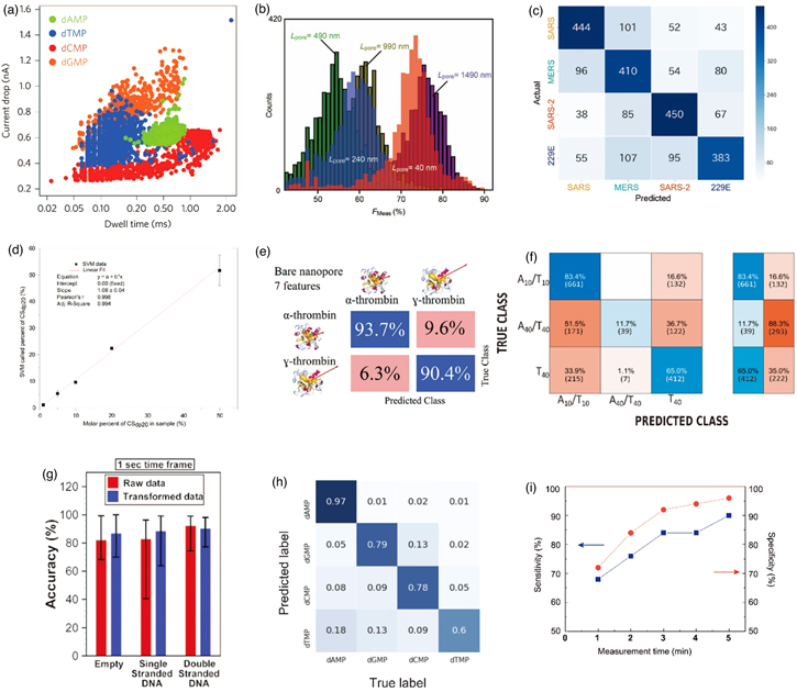
Fig. 7. (Color online) Identification of the analyte molecules. (a) Analysis using typical nonmachine learning. Single-molecule identification employing changes in the current and current duration (four nucleotides were identified). Reprinted with permission from Ref. 28. Copyright 2015 Springer Nature. (b) Identification of E. coli and B. subtilis using Rotation Forest. Histogram of the discrimination accuracy in nanopores exhibiting different thicknesses. Reprinted with permission from Ref. 41. Copyright 2017 Springer Nature. (c) Identifications of four cultured coronaviruses by Random Forest. Confusion matrix resulting from machine learning. Reprinted with permission from Ref. 44. Copyright 2021 Springer Nature. (d) Identifications of two glycosaminoglycan species via SVM. Relationship between the amount of the two glycosaminoglycan species in the mixed solution and the amount estimated by machine learning. Reprinted with permission from Ref. 140. Copyright 2019 American Chemical Society. (e) Identification of proteins via SVM. Confusion matrix obtained by the machine learning of the ionic current–time waveforms of α-thrombin and γ-thrombin. Reprinted with permission from Ref. 141. Copyright 2021 American Chemical Society. (f) Identification of three DNA species employing SVM. Reprinted with permission from Ref. 142. Copyright 2020 MDPI. (g) Identification of three viruses by DNNs. The accuracy of identifying the three viruses: empty indicates adenoviruses that do not encapsulate DNA, and the other two indicate adenoviruses encapsulating single-stranded DNA (ssDNA) and dsDNA. Reprinted with permission from Ref. 143. Copyright 2020. The Royal Society of Chemistry. (h) Identifications of four nucleotide species by DNNs. Confusion matrix obtained via deep learning. Reprinted with permission from Ref. 144. Copyright 2021 American Institute of Physics. (i) Discrimination of the PCR-positive and PCR-negative saliva specimens for SARS-CoV-2 by machine learning. Time dependence of the sensitivity and specificity. Reprinted with permission from Ref. 44. Copyright 2021 Springer Nature.
Download figure:
Standard image High-resolution image
In the machine and deep learning of ionic current–time waveforms, an F-measure is defined as the accuracy with which n analyte molecules can be identified in a single waveform. The F-measure is calculated from the confusion matrix. When the F-measure is 1, the discrimination accuracy is 100%. Thus, n analyte molecules are identified when the F-measure is greater than 1/n. The open library, scikit-learn, 139) is widely employed for machine and deep learning programs. E. coli and Bacillus subtilis were identified with an F-measure = 0.90 via machine learning using Rotation Forest on the ionic current–time waveforms obtained from nanopores exhibiting a diameter of 3 m [Fig. 7(b)]. 41) Cultured SARS-CoV, MERS-CoV, SARS-CoV-2, and HEP-229E have been identified with an F-measure = 0.66 employing Random Forest with nanopores having a diameter of 300 nm [Fig. 7(c)]. 44) Two glycosaminoglycans have been identified using nanopores (diameter = 2.7 nm) and a support vector machine (SVM) with an F-measure of >0.94. 140) In mixed solutions containing both glycosaminoglycan types, machine learning estimated the mixing ratio [Fig. 7(d)]. Using nanopores (diameter = 12 nm) and SVM, α-thrombin and γ-thrombin were identified with an F-measure of 0.93 [Fig. 7(e)]. 141) Three dsDNA consisting of 10 and 40 bases were also identified with an F-measure of 0.82 by SVM with nanopores exhibiting diameters of 2 and 4 nm, respectively [Fig. 7(f)]. 142) Adenoviruses with and without DNA were identified by nanopores (diameter = 100 nm) and deep neural network (DNN) with an F-measure of ≥0.95 [Fig. 7(g)]. 143) Four nucleotides were identified with F-measures of ≥0.94 by MoS2 nanopores with diameters of 2.8 and 3.3 nm, as well as DNN and convolutional NNs (CNN) [Fig. 7(h)]. 144) The measurements also demonstrated the control of the translocation speed of the analyte molecules by IL. These machine learning techniques ensure the accuracy of identifying the analyte molecules obtained using a single ionic current–time waveform.
Clinical saliva specimens that were PCR-positive and PCR-negative for SARS-CoV-2 were measured in nanopores with a diameter of 300 nm at 5 min/specimen. 44) For the training process, 40 PCR-positive and 40 PCR-negative specimens were used, and for the diagnostic process, 50 PCR-positive and 50 PCR-negative specimens were employed. The discrimination accuracy employing Random Forest and positive unlabeled classification (PUC) 145,146) of positive and negative by one ionic current–time waveform was F-measure = 1.00 in the training process. The PUC method learns the ionic current–time waveforms of the impurities in the negative specimens and extracts them from the waveforms obtained from the positive specimens. The ensemble learning of all the ionic current–time waveforms obtained for each specimen exhibited a sensitivity and specificity of 90% and 96%, respectively, for determining the positive and negative results [Fig. 7(i)]. 44)
The machine or deep learning of ionic current–time waveforms can identify a single analyte molecule with high accuracy. Furthermore, clinical specimens can also be identified with high accuracy. The challenges of the practical application include the highly accurate identifications of three or more analyte molecules, as well as the quantitative analysis. Furthermore, the analyte molecules, such as saliva, in the actual sample to be tested must be identified with a high degree of accuracy. Actual samples comprise impurities other than the analyte molecules. Methods have been developed for the removal of impurities by hardware, such as filters and flow channels. There are also methods, such as PUC, for removing impurities by software. Inexpensiveness, high throughput, and ease of operation are required for the practical application of nanopore-based testing and diagnostic methods. Impurity removal can be achieved by fusing hardware and software to satisfy these practical requirements.
6. Outlook
Nanopore clogging accounts for a major challenge to the practical application of nanopores. Even if impurities that are larger than the nanopore can be removed via pretreatment, the adhesion of the analyte molecule causes the clogging of the nanopore. Nanopore clogging is caused by the nonspecific adsorption of the analyte molecules. To prevent this, the nanopore surface can be chemically modified or surfactants can be introduced. 36,147–150) The prevention of nonspecific adsorptions also applies to the channel surfaces leading to the nanopores. Particularly, the prevention of nonspecific adsorptions is key to executing the quantitative analysis of trace amounts of the analyte molecule.
The detection of many types of analyte molecules in a single-chip device represents a challenge to the practical application of multiplex testing and diagnostics. The simultaneous testing of viruses and bacteria of several hundred nanometers and meters, respectively, is highly required for the diagnosis of infectious diseases. 151–155) The detection of viruses and bacteria in a single-chip device requires a multiarray of nanopores with two different diameters. The integration of IC-integrated measurement modules with multiarray structures allows inexpensive, portable nanopore multiarray. 156–158) Multiarraying also contributes to the high throughput of the measurement time. Many ionic current–time waveforms, which ensure high sensitivity and specificity, are required for the determination of the positivity and negativity of a single sample. 44) This indicates that long measurement times are required. Multiarraying can increase the number of ionic current–time waveforms that can be obtained per unit of time. Tests that normally require a measurement time of 5 min for one nanopore can be reduced to three seconds for a multiarray comprising integration of 100 nanopores. This principle can significantly reduce the measurement time.
The nanopore digital platform would be a device that can be connected to smartphones, which have now become a global infrastructure. This has already been demonstrated using next-generation DNA sequencers comprising bionanopores. 159,160) Nanopores with artificial intelligence would facilitate the rapid development of new testing and diagnostic methods by simply changing the diameter of the nanopore, as well as the training data based on the molecule to be analyzed. 44) The output of the test and diagnostic results from the nanopores avail information on when, where, and which type of infection or disease is present in the world. This information would elucidate the dynamics of the spread of infectious diseases, as well as their primary regions. Furthermore, integrated analysis using human flow information could enable localized and effective lockdown based on scientific data.
Acknowledgments
This research was partially supported by New Energy and Industrial Technology Development Organization (NEDO) under Grant No. JPNP19005.
Biographies

Masateru Taniguchi, Ph.D., is a Professor of Bionanotechnology at SANKEN, Osaka University. He obtained a Ph.D. from Kyoto University in 2001. He then became a postdoc at the Institute of Scientific and Industrial Research at Osaka University. In 2002, he became an assistant professor at Osaka University. In 2007, he became a researcher for PRESTO (Precursory Research for Embryonic Science and Technology), Japan Science and Technology Agency. He worked as an associate professor at Osaka University (2008–2011). His current research interests include single-molecule science and single-molecule technologies. In 2013, he founded Quantum Biosystems Inc. to commercialize single-molecule quantum sequencers and was a director of the company. In 2018, he also founded Aipore Inc. and serves on the board of the company to commercialize AI nanopores.