
Abstract
A high-speed, non-contact non-destructive testing method using a scanning airborne ultrasound source and a nonlinear harmonic method has been developed for plate-like structures. The testing time depends on the scanning speed and the number of measurement points. To solve this problem, we propose using compressed sensing with this method. In this paper, we investigated visualizing Lamb wave propagation using the proposed compressed sensing method. In addition, we detected a slit defect by using the Lamb wave propagation image. Our results demonstrated that compressed sensing could be used to reduce the testing time.
Export citation and abstract BibTeX RIS
1. Introduction
Non-destructive testing 1) is used to maintain the safety of large structures, such as chemical plants, power plants and tunnels, and the testing must not interfere with the operation of the structure. Various methods 2,3) have been developed that can quickly and accurately test the condition of structures. Ultrasound testing 4–6) is widely used because of its safety and convenience. Conventional ultrasound testing uses a pulse–echo method, in which the state of the testing target can be identified by irradiating the testing target with ultrasound (bulk waves) from an ultrasound probe and measuring the arrival time of defect echoes. However, because the measurement range is limited to the area directly under the ultrasound probe, testing large structures is lengthy.
Non-destructive testing of large plate structures is performed using the pulse–echo method with Lamb waves. 7,8) Lamb waves 9) are ultrasound waves that propagate longitudinally along the boundary surface over longer distances. For example, 10) a 250 kHz Lamb wave can propagate up to 5 m. Therefore, Lamb waves can test a larger area at a time than bulk waves, and thus using Lamb waves reduces the testing time. However, Lamb waves deform in a complex waveform during the propagation process because of velocity dispersion with respect to frequency and thickness. When the shape of the testing target or defect is complex, it is difficult to identify the defect echo from the received waveform. Consequently, defects may be missed in this method.
To solve this problem, a method for visualizing Lamb wave propagation 11–13) has been proposed that identifies scattering around defects 14) by visualizing Lamb waves propagating inside the testing target. Several visualization methods 15,16) have also been proposed, including the scanning wave source technique, which is based on the sound field reciprocity theorem. In this method, the testing target surface is irradiated with the wave source, the testing area is scanned, and the Lamb waves generated by the irradiation are measured with a fixed receiver. Generally, laser ultrasound 17) is used for the wave source.
A scanning laser source (SLS) technique 18,19) uses ultrasound waves excited by irradiating the testing target surface with low-frequency laser pulses. This method has two advantages: non-contact testing can be performed from a distance by using the laser; and high-speed testing can be performed by laser scanning using mirrors and other devices. However, the target surface can be damaged by melting or evaporation. Furthermore, laser beams are difficult to handle because of the danger of blindness, and thus inspectors must wear light-shielding glasses and safety training is required to use the system.
To overcome these disadvantages, the scanning airborne ultrasound source 20) (SAS) technique has been developed. This method does not damage the target surface because Lamb wave generation requires no contact 21–26) with the test target, and the method is safe because airborne ultrasound is used and equipment handling is easy. In addition, owing to the nonlinear effects of high-intensity sound waves, 20) ultrasound with multiple frequencies (harmonics) can be used simultaneously to perform high-precision testing via nonlinear harmonic methods. High-speed scanning similar to SLS can also be achieved by using an airborne ultrasound phased array. 27–29)
To visualize the propagation of Lamb waves in the SAS method, the propagation waveform from the wave source is measured at each position within the measurement area. The testing time of the scanning wave source technique depends on the wave source scanning speed 19,27) and number of measurement points. Previous studies 27,30) have focused on increasing the scanning wave source speed to achieve high-speed testing. However, reducing the number of measurement points can also speed up conventional testing methods.
One method to reduce the number of measurement points is using compressed sensing, 31–35) which is a signal processing technique that can reconstruct (restore) desired results from minimal experimental results by using sparsity. 36–38)
Testing methods using compressed sensing and Lamb wave visualization have been proposed. 39–41) These methods measure Lamb waves using fixed contact piezoelectric transducers and a scanning laser Doppler vibrometer, which reduces the signal-to-noise ratio due to the surface topography of the testing target and the effects of external disturbances. However, when airborne ultrasound containing nonlinear harmonics is used, the decrease in the signal-to-noise ratio is noticeable. 12,20) Because of these problems, no testing method using compressed sensing and airborne ultrasound with nonlinear harmonics has been proposed.
We have proposed a method for using compressed sensing to reduce the testing time for the SAS method. At USE 2023, 42) compressed sensing was applied to the results obtained using the SAS method, and the Lamb wave propagation image was reconstructed from the small number of measurement results. In addition, the Lamb wave propagation images of each harmonic component were reconstructed using compressed sensing. A reconstructed image was obtained that was comparable to the image constructed using all measurement results. In this paper, we investigate the effectiveness of the proposed testing method by using it to visualize defects.
2. Measurement principle
2.1. Non-contact generation of Lamb waves by airborne ultrasound
In general, when sound waves traveling through air are incident on a solid, it is difficult to generate sound waves in the solid due to the large difference in acoustic impedance between the air and the solid. However, ultrasound waves can be generated in solids by using high-intensity airborne ultrasound. In addition, because of the nonlinear effects of high-intensity airborne ultrasound, sound waves containing harmonics of integer orders of the fundamental frequency can be generated in the solid.
In plate-like solids, the incident sound waves generated are Lamb waves, which have a velocity dispersion with respect to frequency and plate thickness. In addition, Lamb waves have an A mode and S mode, each of which has multiple modes. In thin plates of finite length, Lamb waves are mainly generated in the A0 mode. The velocity of the Lamb wave A0 mode is expressed by the following Rayleigh–Lamb equations 8)


Here, C is the velocity of the Lamb wave,  is the angular frequency, k is the wavenumber,
  is the propagation velocity of the longitudinal wave,
  is the propagation velocity of the transverse wave, and d is the thickness of the plate. In the duralumin plate used in this experiment,
  is 6300 m s−1,
  is 3100 m s−1, and d is 3.000 mm. In addition, the fifth harmonic (209.0 kHz) was used. Under these conditions, from Eqs. (1) to (4), the propagation velocity of the Lamb wave at 209.0 kHz is 2026 m s−1 and the wavelength is 9.692 mm.
2.2. Defect visualization by the Lamb wave propagation image
Figure 1 shows the principle of defect detection and the scattering at the boundary between the healthy area and the slit defect when the Lamb waves are incident perpendicular to the long edge of the slit defect in the metal plate. When the Lamb waves are incident on the slit defect, reflected, transmitted, and diffracted waves are generated near the slit defect. Visualizing these phenomena allows the slit in the thin plate to be detected.
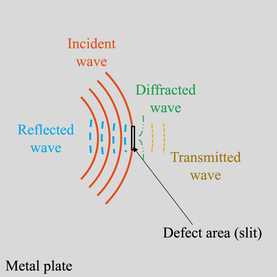
Fig. 1. Overview of defect detection principle.
Download figure:
Standard image High-resolution image2.3. Measurement of Lamb waves in the testing area by the scanning wave source technique
To visualize the wave propagation of Lamb waves, all the time waveforms in a measurement area must be measured. The scanning wave source technique is used to perform this measurement stably. Figure 2 shows the overview of the scanning wave source technique. The scanning wave source technique is performed as follows.
- (1)The measurement position in the testing area is irradiated with a focused airborne ultrasound to generate Lamb waves.
- (2)Lamb waves propagating from each wave source position are measured with the fixed receiver.
- (3)Steps (1) and (2) are followed for the entire testing area. These measurements results are recorded for each of the measurement coordinates.

Fig. 2. Overview of the scanning wave source technique.
Download figure:
Standard image High-resolution imageThis method is less affected by the surface roughness of the testing target because the receiving position can be fixed. In addition, signal averaging processing for the measurements is not required, and the measurement time is shortened. Therefore, measurements can be performed stably and at high speed.
2.4. Applying compressed sensing to the scanning wave source technique
The testing time of the scanning wave source technique depends on the scanning speed and the number of measurement points. However, it is difficult to reduce the testing time by increasing the scanning wave source speed. To solve this problem, a method is needed to reduce the number of measurement points. Therefore, compressed sensing is used to reconstruct Lamb wave propagation images from a small number of measurement data.
In compressed sensing, the measurement process is expressed using simultaneous equations by

where, for the SAS,  is the
  -dimensional original signal when the sampling theorem is satisfied,
  is the
  -dimensional measurement result vector, and
  is the
  measurement matrix. In this simultaneous equation,
  cannot be estimated because
  is less than N due to down-sampling. However,
  can be estimated by using sparsity. In this process, sparse solution x is estimated by using the random down-sampling result, y. In this estimation, the following optimization problem is solved by using the Lagrange multiplier method

Here,  is the Lagrange undetermined multiplier.
The Lamb wave propagation image is not sparse in the image domain. However, x can be transformed into a sparse signal by applying a sparsifying transform matrix,  Through this process, Eq. (6) can be transformed into Eq. (7) as the problem of estimating spatial frequency spectrum

Here,  was
was  x is expressed as

The two-dimensional (2D)-inverse discrete cosine transform (IDCT),
36,43) which is used in reconstruction and compression of images, was used as the sparsifying transform matrix,  We used 2D-IDCT for the following two reasons. First, Lamb waves generated at the sample propagate in a sinusoidal patter, and such waves can be sparsified by discrete Fourier transform (DFT) or discrete cosine transform (DCT). Second, compared with 2D-DFT, 2D-DCT can continuously cycle images and is less likely to generate unnecessary high frequencies.
In this study, the alternating direction method of multipliers (ADMM), 44) which is easy to implement and computationally inexpensive, was used as a proxy method to estimate X from Eq. (7).
2.5. Process flow
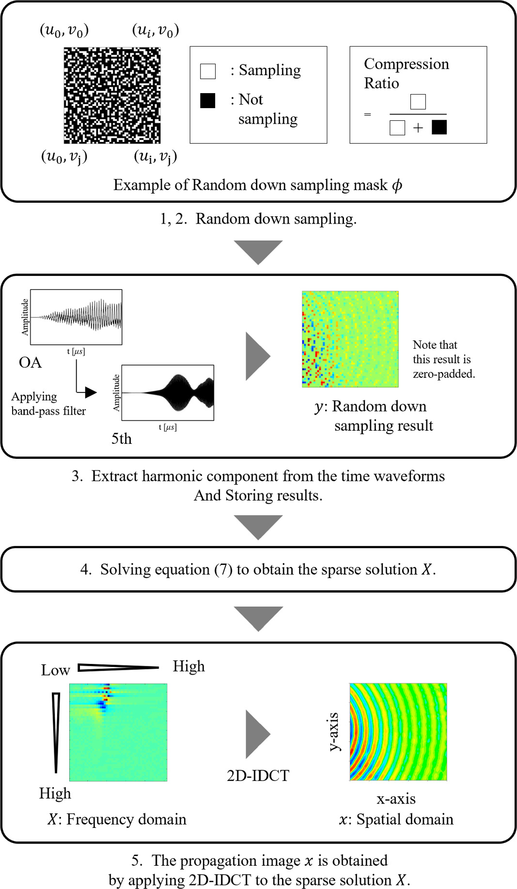
Figure 3 shows a schematic of the compressed sensing process. The flow for reconstructing Lamb wave propagation images from a small number of experimental results by compressed sensing is as follows.
- (1)Setting the number of all measurement points, N, the number of random down-sampling points, M, and the compression ratio,
 based on the measurement area and sampling theorem.
 - (2)Creating a measurement matrix (random sampling mask) according to compression ratio and performing random down-sampling.
- (3)Extracting the harmonic component by applying a band-pass filter to the time waveform of the Lamb wave at each measurement coordinate obtained by random down-sampling. Storing the amplitude information for the time waveform at time t in measurement result (random down-sampling results) y.
- (4)Estimating spatial frequency spectrum X by solving the optimization problem shown in Eq. (7) using random down-sampling results y, random down-sampling matrix and sparsifying transform matrix (2D-IDCT)
- (5)Obtaining reconstructed results of the Lamb wave propagation image by applying 2D-IDCT to X. This process is repeated for each time t to obtain the Lamb wave propagation animation.


Fig. 3. Schematic of the compressed sensing process.
Download figure:
Standard image High-resolution imageIn this study, the random down-sampling results were obtained from the full sampling results to evaluate the reconstructed results obtained by compressed sensing.
3. Overview of the experiment
3.1. Experimental equipment
Figure 4 shows a schematic of the experimental equipment used to verify the proposed method. The equipment consisted of a high-intensity focused airborne ultrasound source (input voltage, 47.0 Vpp; driving frequency, 41.8 kHz; and number of input cycles, 15.0), an acoustic guide, an amplifier (HAS 4051, NF), a synthesizer (WF1974, NF), an acoustic emission sensor (PICO, Physical Acoustics), a preamplifier (2/4/6 C, MISTRAS), a data logger (USB-6363, NI), a three-axis precision stage, and a PC that controlled the peripheral equipment.
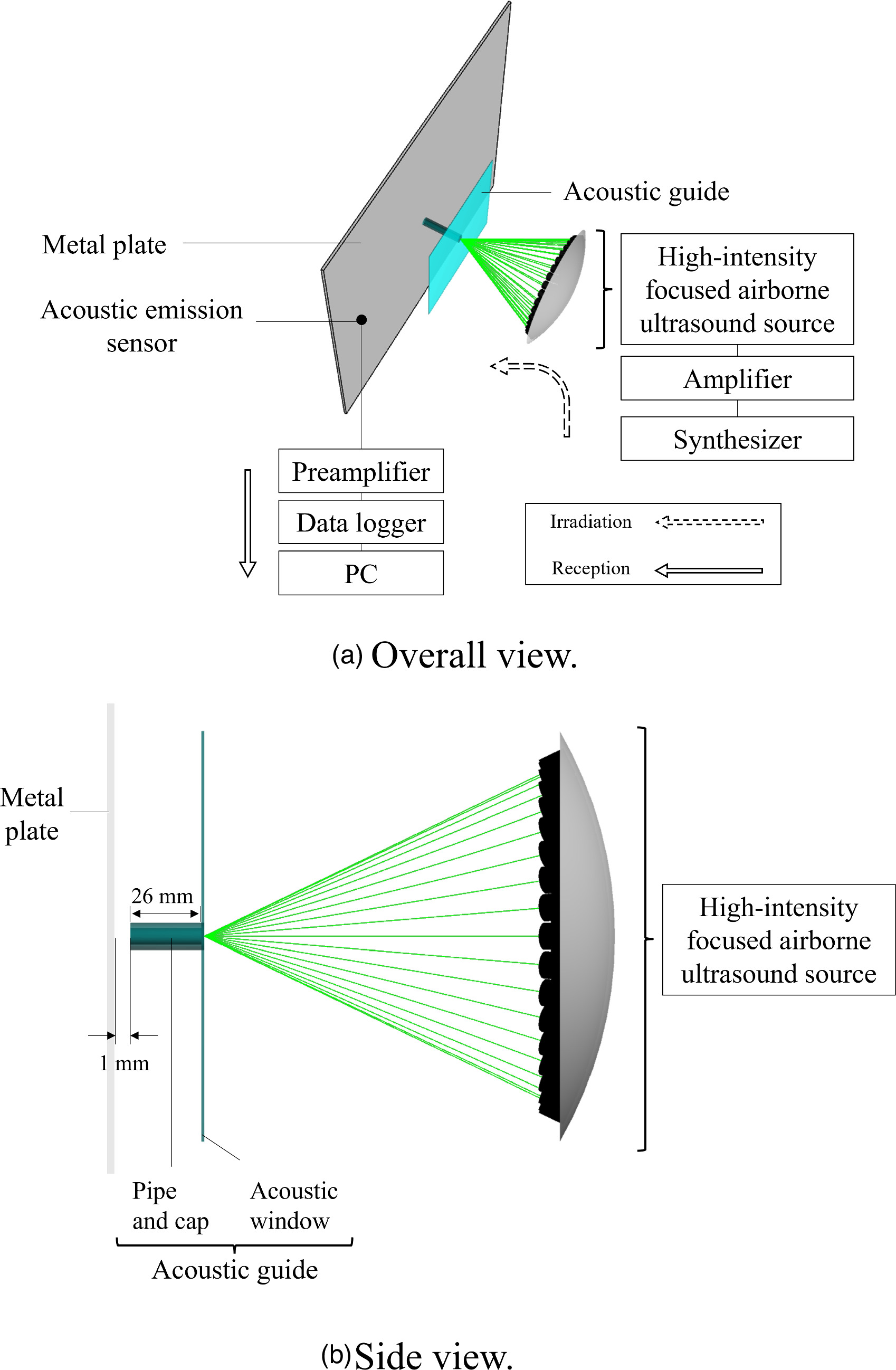
Fig. 4. Schematic of the experimental equipment.
Download figure:
Standard image High-resolution imageThe sound source was composed of 400 ultrasound emitters arranged on part of a spherical surface, with a focusing distance of 150 mm. In addition, to prevent the effects of side lobes, the sound waves were irradiated through an acoustic guide consisting of an acoustic window (acrylic; thickness, 5.0 mm) and a pipe with 2.0 mm hole cap attached to the end (acrylic; length, 26.0 mm; inner diameter, 6.0 mm).
Figure 5 shows the sound pressure distribution after passing through the acoustic guide. This result was measured with an 1/8 in. microphone (40DP, GRAS Sound and Vibration). The results confirmed that high-intensity airborne ultrasound with a maximum sound pressure of 11.1 kPa was generated and that the airborne ultrasound radiated in circle with a diameter of 2.80 mm. Because of the nonlinear effects of high-intensity airborne ultrasound, 12,20,28) the radiated sound wave contained integer-order harmonics.
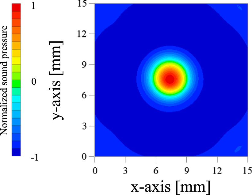
Fig. 5. Sound pressure distribution.
Download figure:
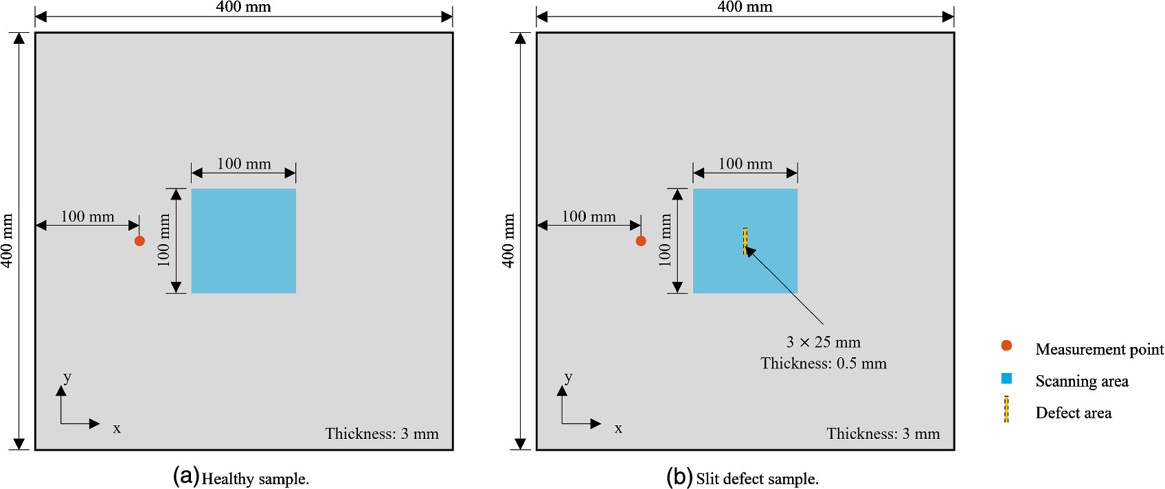
Standard image High-resolution imageFigure 6 shows a schematic of the healthy sample [Fig. 6(a)] and the slit defect sample [Fig. 6(b)] used in the experiment. The samples ware made of plate-like duralumin. The dimensions of each sample were 400.0 × 400.0 × 3.0 mm, and the dimensions of the slit defect were 3.0 × 25.0 × 0.5 mm.

Fig. 6. Schematics of the samples.
Download figure:
Standard image High-resolution image3.2. Experimental conditions
To verify the proposed method, the compression ratio was selected based on the full sampling conditions as follows. The full sampling conditions are the conditions for reproducing the wavefield of the Lamb wave propagating in the metal plate. When defects are targeted, the conditions should visualize the defects. Previous studies 12,20) have shown that the slit defects used here can be detected using ultrasound with a frequency of 200 kHz. The slit defect can be visualized by setting the scanning step to 2.0 mm for the short side (3.0 mm) of the slit defect. Therefore, the measurement interval under full sampling conditions was set to 2.0 mm.
The compression ratio is related to the reduction in measurement time and the accuracy of reconstruction. As the compression ratio increases, the measurement time is reduced; however, the amount of data available for reconstruction decreases. This reduction in data makes it difficult to reconstruct the desired Lamb wave propagation image, especially when targeting defects. Obtaining information on defects is crucial for accurate reconstruction. Therefore, there is a need to consider the optimal compression ratio that can visualize defects while minimizing measurement time. However, since each defect varies in size and random down-sampling is conducted, it is not possible to determine the optimal compression ratio for reconstruction in advance.
For these reasons, this study examined the optimal compression ratio by evaluating the reconstruction results at various compression ratios. We determined the optimal compression ratio by prediction based on the positional relationship between the slit defect and full sampling conditions.
Figure 7 shows the relationship between the full sampling conditions and the position of slit defects. The white pixels indicate the full sampling points. The yellow area indicates the defect location. The red dot indicates the location where the slit defect was measured under the full sampling conditions.

Fig. 7. Relationship between full sampling conditions and slit defect position.
Download figure:
Standard image High-resolution imageFirst, under the full sampling conditions of this paper, 13 points can be measured for a slit defect as shown in Fig. 7. If all 13 points can be measured, defects can be visualized. However, since the positions of these 13 points are not known in advance, it is necessary to perform measurements at points other than the 13 points. Next, measurements must be performed randomly. However, if measurements are performed randomly across all measurement areas, bias may occur. To prevent this, random down-sampling uses jitter sampling, 42) in which the measurement area is divided into small blocks, and the number of measurement points is assigned so that each block has the same compression ratio. This prevents bias from occurring across the entire measurement area.
Based on the above, we can qualitatively predict the optimal compression ratio. In Figs. 7, 9 points (3 × 3) are divided into 1 block. For one block, there are three points of defect information. Therefore, if the compression ratio is set to 66.7%, which measures 3/9 of the total, it is possible to reconstruct the defects. However, not all three points fall within the defect area, so the compression ratio needed to reconstruct the defect is anticipated to be less than 66.7%. Therefore, to determine the optimal compression ratio, we conducted verification within a range that encompasses a compression ratio of 66.7%. Specifically, we considered a range from 88.9% (1/9) to 86.0%, 84.0%, 82.0%, 80.0%, 77.8% (2/9), 76.0%, 74.0%, 72.0%, 70.0%, 66.7% (3/9), 66.0%, 64.0%, 62.0%, 60.0%, 58.0%, 55.6% (4/9), 54.0%, 52.0%, and 50.0%. In addition, to assess the variation resulting from random down-sampling, we examined the reconstructed results of 50 patterns at each compression ratio.
In this measurement, the sound waves irradiated from the pipe aperture end were scanned two-dimensionally at each position within the measurement area, and the generated Lamb waves were received by the acoustic emission sensor installed in the fixed position.
Figure 6 shows the measurement area. The measurement area was 100 × 100 mm at the center of the sample, the scanning step of the wave source was 2.00 × 2.00 mm, the sampling frequency was 2.00 MHz, and the sampling time was 5.00 ms. Hereafter, the experimental results obtained under these measurement conditions are called the full sampling results.
3.3. Experimental method
For the received waveforms, the following processing was performed to apply compressed sensing. First, random down-sampling results were obtained by spatially decimating the data from the full sampling results using the method described in Sects. 2.5 and 3.2 for comparison with the full sampling results. Next, the Lamb wave propagation images were estimated by using the method described in Sect. 2.5.
4. Results and discussion
The reconstructed results were evaluated according to the following policy. The proposed method identified defects by focusing on the scattering of Lamb wave propagation near the defect. At this time, the phase information about the spatial waveform in the healthy area and the amplitude information from the slit defect area were important. Therefore, the reconstructed results were subjectively compared and evaluated with the full sampling results, focusing on phase and amplitude changes. In addition, we compared and evaluated the correlation coefficient between the full sampling results and the reconstructed results.
4.1. Reconstructed Lamb wave propagation image in the healthy sample
Figure 8 shows Lamb wave propagation images of the healthy sample at each compression ratio (88.9%–50.0%). Figures 8(a)–8(t) shows the reconstructed results, and Fig. 8(u) shows the full sampling result. Figure 8(v) shows the legend. The figure shows the time when 10 wavelengths of the Lamb waves are visible in the propagation image. The results are normalized to their maximum values. We visually evaluate the results.
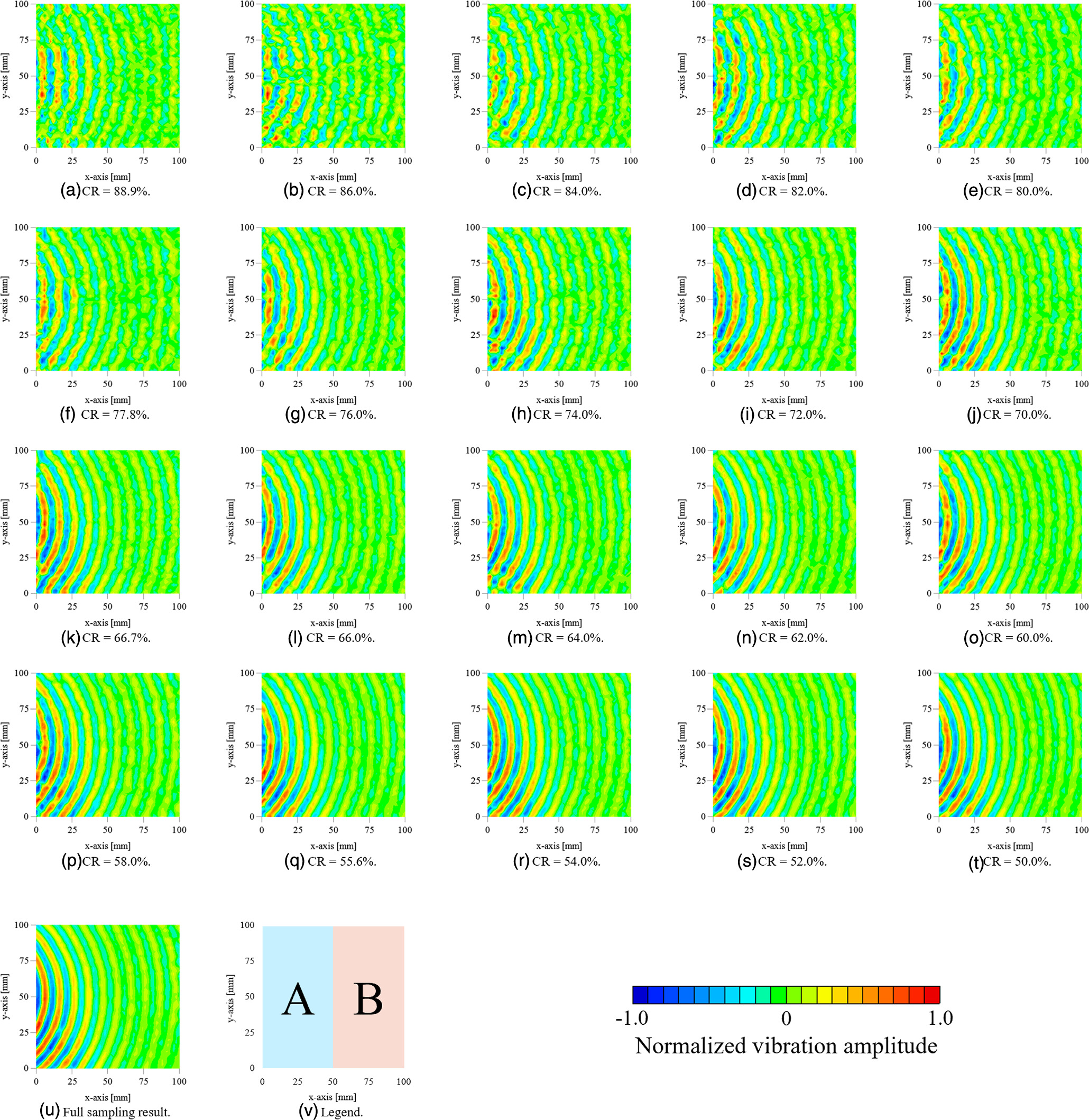
Fig. 8. Lamb wave propagation images (healthy sample).
Download figure:
Standard image High-resolution imageThe full sampling result [Fig. 8(u)] confirmed the propagation of spherical waves (Lamb waves) from the wave source. Analysis of the wavefront confirms that there is no discontinuity in the area A [Fig. 8(v)]. In the B area [Fig. 8(v)], it can be confirmed that the amplitude value decreases due to diffusion attenuation.
Next, we considered the reconstructed results [Figs. 8(a)–8(t)] as follows. In Figs. 8(a) and 8(b), it could not be confirmed that spherical waves are propagating from the wave source. In Figs. 8(c)–8(h), discontinuity occurred in area A, but spherical waves were propagating. In Figs. 8(i)–8(t), no discontinuities were observed on the wavefront, and spherical waves were propagating.
4.2. Reconstructed Lamb wave propagation image of the sample with the slit defect
Figure 9 shows Lamb wave propagation images of the slit defect sample at each compression ratio (88.9%–50.0%). Figure 9(a)–(t) shows the reconstructed results, Fig. 9(u) shows the full sampling result, and Fig. 9(v) shows the legend. The figure shows the time when 10 wavelengths of the Lamb waves are visible in the propagation image. The results are normalized to their maximum values. We visually evaluated the results.
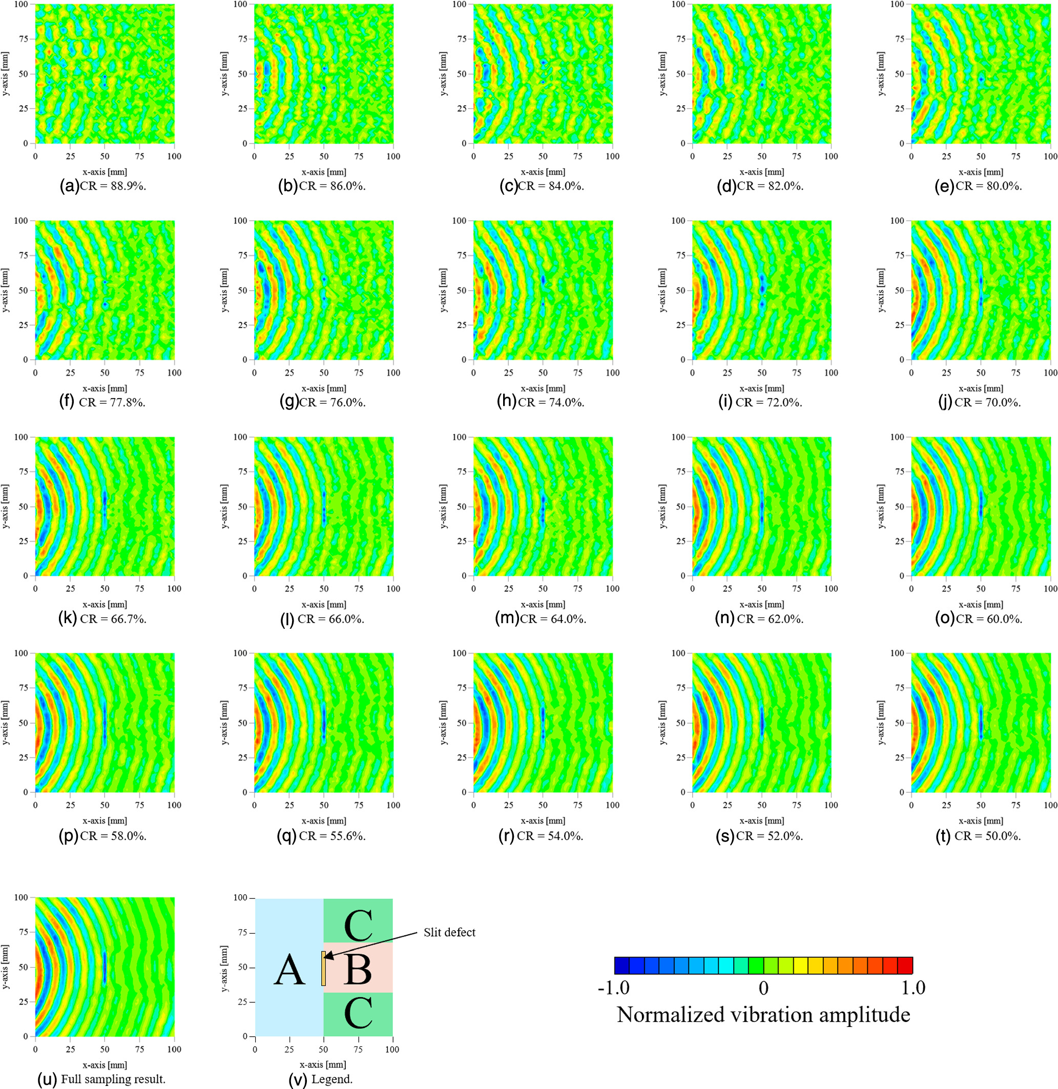
Fig. 9. Lamb wave propagation images (slit defect sample).
Download figure:
Standard image High-resolution imageFirst, we consider the full sampling results [Fig. 9(u)]. The results confirmed that spherical waves (Lamb waves) propagated from the wave source. In addition, in area B [Fig. 9(v)], the Lamb wave incident on the slit defect was diffracted after passing through the slit defect, and the phase delay was confirmed. The amplitude in the slit defect area was lower than in the healthy area. Therefore, slit defects were confirmed visually from the full sampling results.
We discuss the reconstructed results as follows. We focus on the slit defect area and area B [Fig. 9(v)]. In Figs. 9(a)–9(h), the diffraction waves around the slit defect were not visible and it could not be confirmed that the amplitude of the defective area was lower than that of area A [Fig. 9(v)]. In Figs. 9(i)–9(m), the amplitude of the slit defect area was lower than that of area A [Fig. 9(v)]. However, in area B [Fig. 9(v)], no diffraction waves were visible. In contrast, in Figs. 9(n)–9(t), the diffraction waves around the slit defect area were visible and the amplitude value was lower in the slit defect area than in the healthy area. Therefore, the slit defect was visually confirmed in Figs. 9(n)–9(t).
4.3. Evaluation of the proposed method using the correlation coefficient
Correlation was used to compare and evaluate the Lamb wave propagation images obtained by the proposed method. The correlation coefficient was obtained using the following formula

Here,  is the full sampling result,
  is the average value of the full sampling result,
  is the reconstructed result, and
  is the average value of the reconstructed result.
  is a correlation coefficient and takes a value between −1.00 and 1.00.
Note that there is no universal standard for correlation coefficients. This is because the required correlation coefficient varies depending on the target signal and information. In this work, we used 0.9 as a standard for evaluation based on research by Mesnil and Ruzzene, 41) and we confirmed its consistency with visual assessments.
Figure 10 shows the correlation coefficient for each compression ratio. The blue line shows the healthy sample, and the red line shows the slit defect sample. The evaluation was for compression ratios of 88.9%–50.0%. In addition, to evaluate the variation due to random down-sampling, we verified 50 patterns at each compression ratio, and thus the results show the average of 50 correlation coefficients at each compression ratio. The error bars are based on the standard deviation of 50 correlation coefficients at each compression ratio.

Fig. 10. Correlation coefficient (R) with increasing compression ratio. The error bars indicate the standard deviation of the correlation coefficients for the 50 patterns.
Download figure:
Standard image High-resolution image
First, we focus on the average value of the correlation coefficient. The correlation coefficient decreased as the compression ratio increased. For compression ratios of 84.0% or higher, the correlation coefficient of the healthy sample was larger than that of the sample with a slit defect. In addition, the compression ratio with a correlation coefficient of 0.900 or higher was 66.7% or less in both results.
Next, we focus on the standard deviation of the correlation coefficient. The standard deviation increased as the compression ratio increased. For a compression ratio of 88.9%, the correlation coefficient was 0.0506 for the healthy sample and 0.0502 for the slit defect sample. For a compression ratio of 66.7%, where the average value of the correlation coefficient was 0.900 or more, the standard deviation was 0.0119 for the healthy sample and 0.0116 for the slit defect sample.
These results indicate that as the compression ratio increased, the full sampling and reconstructed results did not match. In addition, as the compression ratio increased, the standard deviation increased, indicating greater variability in the performance of the proposed method.
We compare the visual evaluation in Sects. 4.1 and 4.2 and the correlation coefficients. For the healthy sample, the correlation coefficient was less than 0.900 at a compression ratio of 74.0% or higher, where discontinuities were found in the wavefront. When the compression ratio was between 72.0% and 70.0%, Lamb wave propagation was visually confirmed, but the correlation coefficient was less than 0.900. For the slit defect sample, the slit defects could not be distinguished visually at compression ratios greater than 70.0%, and the correlation coefficient was less than 0.900. When the compression ratio was between 66.7% and 64.0%, no diffracted wave propagation was observed in area B. However, the correlation coefficients were greater than 0.900. Therefore, based on the visual evaluation and correlation coefficients, we determined that reconstruction was not possible with the compression ratio of 64.0% or higher, and with compression ratios in this range, defects could not be reliably identified.
At compression ratios of 62.0% or less, where the slit defect and diffraction waves were observed, the correlation coefficient was 0.900 or higher. Therefore, the optimal compression ratio for identifying slit defects using the proposed method was 62.0% or less. In other words, the proposed method suggested that the testing time for conventional SAS 20,28) could be reduced by up to 62.0%. These results demonstrated that the proposed method was effective in visualizing slit defects.
The difference between the reconstructed results (amplitude and phase information) and the full sampling results was probably caused by the random down-sampling. 39,40) In this paper, we used compressed sensing that focused on only the spatial information of the Lamb waves. If defect information is included in the acquired spatial information, the slit defect can be reconstructed using the proposed method. However, whether the spatial information contains defect information depends on the random down-sampling. For example, in the slit defect and full sample conditions of this paper, measurements were taken at 13 points for the slit defect, as shown in Fig. 7. If all 13 points can be measured, defects can be visualized in the same way as the full sampling results. However, because the number of measurement points is reduced by random down-sampling, it is not possible to measure all 13 points. Consequently, some defect information is lost, causing error in the amplitude value of the defect area. For other conditions, the amount of defect information required varies depending on the defect size and wavelength, so the defect reconstruction accuracy changes. In future work, the performance of the proposed method should be improved by using time information in addition to the spatial information for the Lamb wave to address this problem.
5. Conclusion
We proposed a scanning airborne ultrasound source technique using compressed sensing. To confirm the effectiveness of the proposed method, we investigated the following points.
First, we visually evaluated the reconstructed results of Lamb wave propagation images in the healthy sample and the slit defect sample. Next, we investigated the effective compression ratio of the proposed method by comparing the correlation coefficient and visual evaluation. For slit defects, it was similarly effective in less than 62.0% of cases, but the random down-sampling pattern caused differences from the full sampling results. In future work, the proposed method should be improved to achieve better performance.
Acknowledgments
This work was partly supported by JSPS KAKENHI Grant No. 22K04624.