
Abstract
To enable quantitative assessments of multi-directional blood flow dynamics such as those in the heart, a two-dimensional (2D) flow vector estimation method using dual-angle Doppler measurements with a sector ultrasound probe was developed. However, that technique was prone to aliasing artifacts because the dual-angle transmissions reduced the pulse repetition frequency (PRF) and Nyquist flow speed by half for each Doppler measurement. To overcome this problem, this study devised a new dual-angle vector flow imaging framework with extended Nyquist velocity using the dual-PRF de-aliasing method. In the proposed framework, the Nyquist flow speed was doubled to 930 mm s−1 compared with the conventional dual-angle approach. Imaging experiments demonstrated that the proposed framework could correct the aliasing artifacts in color Doppler frames and successfully derive 2D flow vectors comparable to particle image velocimetry measurements with a relative error of −14.5% in the fast and 35.2% in the slow flow phases in a pulsatile flow condition.
Export citation and abstract BibTeX RIS
1. Introduction
The global prevalence of ischemic heart disease (IHD) is increasing, and it is considered to be one of the leading causes of mortality. 1,2) IHD involves the narrowing of the lumen of coronary arteries, which reduces the blood supply to cardiac muscles. Although there have been dramatic developments in the emergency management of IHD through percutaneous coronary intervention since the 1990s, heart failure is still a critical complication of myocardial infarction. Earlier and proper diagnoses may reduce the adverse events of the disease and the death ratio. Traditionally, blood flow measurements in the chambers of the heart have been recognized as diagnostic indicators when assessing cardiac function. In this regard, ultrasound color Doppler imaging (CDI) has been widely used in cardiology as one of the most essential and noninvasive modalities. It has high temporal resolvability and real-time capability, which are not provided by other flow imaging modalities such as magnetic resonance imaging (MRI) and computed tomography (CT). 3–10) Despite the usefulness of CDI, the complexity of the flow dynamics in the heart's chambers often hampers a quantitative investigation of the one-dimensional (1D) blood flow speed obtained with conventional CDI techniques. Therefore, estimating two-dimensional (2D) flow velocities has been considered a potential solution to enable more quantitative and precise assessments of the complex hemodynamics in the heart.
To date, various 2D flow velocity estimation methods such as speckle tracking, 11–13) vector flow mapping (VFM), 14,15) echo-dynamography (EDG), 16–18) and two-angle vector Doppler measurements have been reported to visualize the flow dynamics in the heart's chambers. 19) The speckle tracking method was computationally expensive and degraded by the out-of-plane motion, and the VFM and EDG methods utilized assumptions about the fluid dynamics that were sometimes affected by noise components in CDI. On the other hand, the two-angle vector Doppler method, which we reported previously, 19) estimated 2D flow vectors based on the trigonometric relationships between two 1D flow components obtained by transmitting diverging waves from two different angles. This did not require any flow dynamics assumptions and could effectively derive the 2D vectors at a low computational cost.
Nevertheless, the dual-angle vector Doppler method could reduce the possible pulse repetition frequency (PRF) in the respective directions by half and make the Doppler estimations prone to aliasing artifacts. When the flow direction in the imaging field was constant, the aliasing artifacts could be readily corrected by unwrapping the phase information, but in the present scenario of multi-directional flow measurement, identifying aliased regions could be difficult. If those aliasing artifacts remained in the CDI data, they could estimate inaccurate 2D flow vectors. To overcome the problem and enable robust 2D flow vector estimations for echocardiography, our present study devised a new framework for combining the dual-angle vector Doppler method with a dual-PRF transmission scheme, which could extend the Nyquist speed of CDI for each transmission angle. In a preliminary study, 20) we evaluated the performance of the dual-PRF adaptive de-aliasing method in diverging imaging with a sector probe by measuring a constant flow in a straight lumen phantom and confirmed that the dual-PRF approach provide aliasing-free CDI that was equivalent to the conventional single-PRF CDI with manual phase unwrapping de-aliasing.
Based on these observations, in the present study, we further investigated the performance of the dual-PRF, dual-angle vector Doppler imaging method. For that purpose, we performed an imaging experiment using a sector probe on a custom-made flow phantom with both constant and pulsatile flow. The 2D flow vectors were calculated using the acquired data and evaluated in comparison with flow velocities measured using particle image velocimetry (PIV), 21,22) which is an optical modality to measure 2D velocity vectors.
2. Methods
In the proposed imaging framework (dual-PRF, dual-angle vector Doppler), leveraging ultrafast diverging imaging techniques, four color Doppler datasets (from the combinations of two PRFs and two transmission angles) were acquired for each flow vector image frame. First, two pairs of color Doppler datasets obtained using the same transmission angle were used to adaptively correct the aliasing artifacts based on the dual-PRF de-aliasing principle. 23) This process generated two "aliasing-free" color Doppler datasets corresponding to the respective transmission angles. Second, those dual-angle color Doppler datasets were used to calculate flow vectors. 24) Finally, obtained vectors were visualized on a B-mode image simultaneously acquired with the Doppler frames.
2.1. Dual-PRF de-aliasing method
The Nyquist velocity  in the color Doppler method is given by Eq. (1):

where  is the wavelength of the acoustic pluses. In the dual-PRF method, two different PRFs (PRF1 and PRF2) are selected, where PRF1 is defined based on the imaging depth and expected maximum flow velocity, while PRF2 is set as shown in Eq. (2):

where  and
and  are mutually prime numbers and
  In addition, the relationship between the Nyquist speeds,
  and
and  , can be derived as follows:

In this study, we used a condition,  and
and  As illustrated in Fig. 1, the Doppler shifts measured with the respective PRFs aliased at their respective Nyquist speeds and showed the relationships between the actual and measured velocities. Each color-coded region in Fig. 1 shows a unique difference between the flow speeds measured by
  and
and  and can be identified using the Eq. (4):

where  and
and  are the flow speeds measured at the respective PRFs, and the
  function gives the closest integer value. The value of
  calculated in Eq. (4) was used to obtain the number of aliased cycles (Nyquist numbers,
  ) at each pixel in the color Doppler frames measured with the respective PRFs, as listed in Table I. Finally, the Nyquist numbers,
  and
and  , were substituted into Eq. (5) to calculate the de-aliased Doppler velocity,

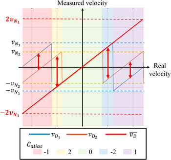
Fig. 1. (Color online) Relationship between flow velocity to be measured at two respective pulse repetition frequencies, and flow velocity after de-aliasing. Red arrows indicate the differences between the flow velocities measured at respective PRFs that are used to identify  number.
Download figure:
Standard image High-resolution imageTable I. The Nyquist numbers (number of aliasing cycles for each PRF measurement) determined by different  values.

|

|

|
|---|---|---|
| 2 | 0 | −1 |
| 1 | 1 | 1 |
| 0 | 0 | 0 |
| −1 | −1 | −1 |
| −2 | 0 | 1 |
As shown in Fig. 1, the Nyquist speed of the dual-PRF color Doppler could be increased to twice the original Nyquist speed, 
2.2. Calculation of 2D flow vectors
After the dual-PRF de-aliasing was performed, aliasing-free color Doppler frames for each transmission angle were obtained. At each pixel in those frames, the flow speed components along each transmission angle,  and
and  were used to compute the 2D flow vectors. Fig. 2(a) illustrates the geometric relationships between the transmitted diverging waves and the measured and de-aliased flow speed components. The actual 2D velocity components along the x and z axes,
  and
and  could be decomposed as shown in Figs. 2(b) and 2(c) using
  and
and  and those relationships can be expressed as Eqs. (6) and (7):


where  and
and  are the transmission angles and should be calculated at each pixel because of the nature of the diverging wave. Finally, from Eqs. (6) and (7), the components of the 2D velocity vector (
 ) are derived as follows:


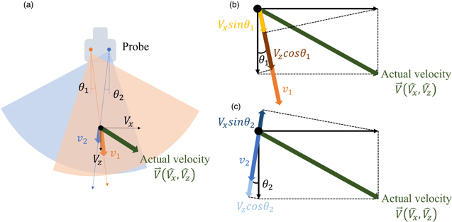
Fig. 2. (Color online) (a) Illustration of transmission of dual-angle diverging waves from a sector probe, and (b) and (c) geometric relationships between the actual flow velocity and flow velocity measured from the first and second transmit directions, respectively.
Download figure:
Standard image High-resolution image2.3. Evaluation of dual-PRF de-aliasing in diverging wave imaging
First, we evaluated the de-aliasing performance of the proposed dual-PRF, dual-angle flow measurement scheme because, as discussed in Sect. 2.2, it was important to accurately estimate the 1D flow speed in the color Doppler method to achieve accurate and robust estimations of the 2D velocities. The imaging system was comprised of a research-purpose ultrasound system (Vantage 256 system, Verasonics Inc., USA) equipped with a custom sector probe (64 channels, center frequency: 2.5 MHz). The flow phantom (Doppler 403 Flow Phantom, Model 1425B, GAMMEX, USA) had a straight flow channel with an inner diameter of 5 mm sloped at  (Fig. 3). Two flow conditions were used (a constant flow of 8.0 ml s−1 and pulsatile flow of 12 ml s−1 at 60 bpm). In this study, the flow signals obtained from the flow channel at a depth of 5–8 cm (indicated as the red region in Fig. 3) were processed and visualized by manually setting the region of interest (RoI) based on a power Doppler image.

Fig. 3. (Color online) The geometry of the flow tract in the Doppler 403 Flow phantom. The region in red indicates the flow region to be visualized.
Download figure:
Standard image High-resolution imageWe designed an imaging sequence for the dual-PRF, dual-angle scheme (Fig. 4) using the detailed imaging parameters listed in Table II. First, a B-mode dataset was acquired by emitting 15 diverging wave pulses (Tx angle range:  –
– ). Second, the dual-PRF Doppler sequence was performed as indicated by the yellow and green boxes in Fig. 4. In each block, thirty-four diverging wave pulses were alternatively emitted from
  The PRF for the first and third blocks was set at 2.0 kHz
  while that of the other blocks was at 1.3 kHz
  In each data acquisition, 10 frames of data (B-mode and flow vector) were acquired for the constant flow measurements, and 100 frames were acquired for the pulsatile flow measurements.
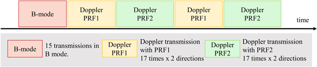
Fig. 4. (Color online) Transmission sequence for acquiring a frame of the dual-angle, dual-PRF vector Doppler imaging.
Download figure:
Standard image High-resolution imageTable II. Ultrasound imaging parameters for the dual-PRF, dual-angle imaging framework.
| Parameters | Values |
|---|---|
| Probe | Sector |
| Center frequency [MHz] | 2.5 |
| Channel number | 64 |
| B-mode | |
| PRF [kHz] | 4.5 |
| Number of transmissions | 15 |
| Range of transmission angle [°] |

|
| Pulse length | 1 pulse |
| Doppler | |
| PRF1 [kHz] | 2.0 |
Nyquist speed  [mm s−1] [mm s−1] | 310 |
| PRF2 [kHz] | 1.3 |
Nyquist speed  [mm s−1] [mm s−1] | 207 |
| Extended Nyquist speed [mm s−1] | 620 |
| Pulse length | 3 pluses |
| Ensemble size | 65 |
| Transmission angles [°] |

|
| Frame rate [fps] | 20 |
| Imaging depth [cm] | 13.5 |
The acquired data were processed in a pipeline, as shown in Fig. 5. For the Doppler measurements at each PRF setting, the acquired echo data were processed using a singular value decomposition clutter filter and a lag-1 autocorrelator to generate color Doppler images.
25–27) The aliasing artifacts in the color Doppler images obtained with the different transmission angles were corrected with the dual-PRF de-aliasing framework described in Sect. 2.1 using data obtained with two PRF conditions. To compare the de-aliasing performance of the dual-PRF method with that of the conventional manual phase unwrapping approach (hereafter, the single-PRF method), we used color Doppler data acquired at  and manually de-aliased by applying Eq. (10) to all of the negative speed values:


Fig. 5. Data processing pipeline for visualizing de-aliased color Doppler images and 2D flow vectors.
Download figure:
Standard image High-resolution imageAfter performing the respective de-aliasing methods, the estimated flow speed maps were processed with a temporal (9 frames) and spatial (6  6 pixels) smoothing filter.
2.4. Verification of the robust 2D flow vector estimation
To verify the accuracy of the 2D velocity vector estimation using the proposed imaging framework, another flow phantom experiment was conducted to measure the same flow with ultrasound and a PIV system (Kato Koken Co., Ltd., Japan). Figure 6 illustrates the setup used in this experiment. The straight flow channel phantom had an inner diameter of 8 mm and was made of PVA-gel.
28–30) It is important to note that this PVA-gel phantom was both acoustically and optically transparent. Thus, the ultrasound and PIV methods could measure the same flow profile. The blood mimicking fluid (BMF) used as the liquid in the flow phantom consisted of distilled water, spherical silica particles (Godd ball, Suzukiyushi Industrial Co., Ltd., Japan) as an acoustic scatterer, and polyamide seeding particles (PSP-50, DANTEC, Denmark) as a PIV tracer. To circulate the BMF, the phantom was placed in a water tank and connected to a custom gear-flow pump to generate a constant flow of 18 ml s−1 or a pulsatile flow of 21 ml s−1 at 60 bpm. For ultrasound imaging, a sector probe was placed above the phantom at a tilt angle of  [Fig. 6(a)]. For the PIV measurement, a laser sheet and high-speed camera were used to acquire the flow profile on the same imaging plane as the ultrasound imaging [Fig. 6(b)]. The high-speed camera captured the motion of the tracer particles at 1000 fps, and the 2D flow vector field was calculated using commercial PIV software (Flow Expert 2D2C, Kato Koken).
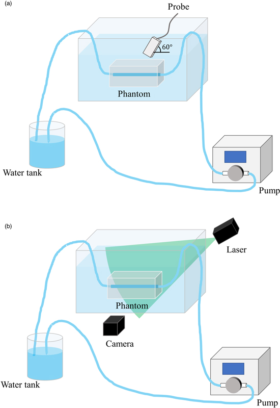
Fig. 6. (Color online) Experiment setup for comparing ultrasound and PIV measurements. (a) The position of the ultrasound probe, and (b) the positions of the laser sheet and the high-speed camera for PIV measurement.
Download figure:
Standard image High-resolution imageIn this experiment, we used PRF values (3.0 kHz for PRF1 and 2.0 kHz for PRF2) to acquire images at a depth of approx. 10.2 cm (Table III) and processed the acquired echo data with the data processing pipeline shown in Fig. 5. In addition to the dual-angle, dual-PRF flow velocity estimation, we also performed 2D flow velocity estimation using the dual-angle color Doppler data measured at PRF1 without any aliasing correction to verify the efficacy of the proposed method.
Table III. PRFs and their Nyquist speed values used for the experiments to compare the 2D flow vectors estimated with the proposed and PIV measurements.
| Parameters | Values |
|---|---|
| PRF1 [kHz] | 3.0 |
Nyquist speed  [mm s−1] [mm s−1] | 465 |
| PRF2 [kHz] | 2.0 |
Nyquist speed  [mm s−1] [mm s−1] | 310 |
| Extended Nyquist speed [mm s−1] | 930 |
| Pulse length | 3 pluses |
| Ensemble size | 65 |
| Transmission angle [°] |

|
| Frame rate [fps] | 27 |
| Imaging depth [cm] | 10.2 |
3. Results and discussion
3.1. Evaluation of dual-PRF de-aliasing in diverging wave imaging
Figures 7(a) and 7(b) show examples of the obtained color Doppler images (transmission angle: −30°) under the different PRF conditions in the constant flow setting. Because of the variation in the diverging beam direction [Fig. 7(c)], the measured flow speed and appearance of the aliasing artifacts in the color Doppler images changed with the depth. For example, the beam directions at the red and white points in Fig. 7(c) were 2.4° and 17.5°, respectively, and the angles between the beam direction and the flow direction (40°) were 47.6° and 32.5°, respectively. As such, in this imaging scenario, the measured flow speed continuously increased from the upper part to the bottom part in the flow region, and aliasing artifacts occurred when the measured flow speed exceeded the Nyquist velocity of respective PRFs [Figs. 7(a) and 7(b)]. Using those color Doppler images, aliasing-free color Doppler images were generated based on the dual-PRF de-aliasing approach [Fig. 7(d)] and showed profiles similar to those obtained with the single-PRF method [Fig. 7(e)]. The percentage errors between the images de-aliased with the dual-PRF and single-PRF methods [Fig. 7(f)] also showed high similarity between the two methods, and the mean absolute percentage error was found to be 21.5%. In the upper right region of the flow tract, where the angle between the acoustic beam and flow direction was high and the measured flow speed was small, it was observed that the errors between the dual-PRF and single-PRF methods were quite small, whereas in the lower left region of the tract, where the measured flow speed was high, the error values were larger.
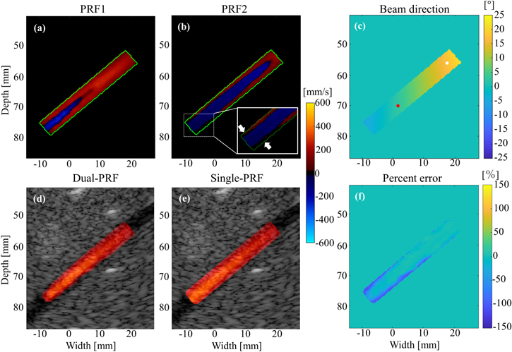
Fig. 7. (Color online) Color Doppler images of the constant flow setting from the transmission angle of  measured at (a) PRF1 and (b) PRF2, respectively. The green box shows the RoI used in the experiment. (c) The ultrasound beam directions at each pixel in the flow region. (d) and (e) The de-aliased color Doppler image processed with the dual-PRF and single-PRF approaches, respectively. (f) The percent error map between (d) and (e).
Download figure:
Standard image High-resolution imageThe de-aliasing performance of the proposed framework was also evaluated in the pulsatile flow condition. Figures 8(a)–8(d) shows the color Doppler images (transmission angle of  ) acquired at slow and fast flow phases in a cycle of pulsatile flow. Similar to the constant flow images, a higher flow speed was measured in the lower left region, corresponding to the beam direction [Fig. 8(k)]. In the fast flow phase, color Doppler images in both PRF conditions [Figs. 8(b) and 8(d)] had aliasing artifacts. Particularly in PRF2 condition [Fig. 8(d)], the flow velocity was measured to be positive without aliasing in the upper right area, aliased to the negative with one-cycle of aliasing in the middle area, and finally increased to the positive value with one-cycle of aliasing in the lower left area. This observation could also be found in the flow velocity profile shown in Fig. 8(l). With this setting, the dual-PRF method effectively corrected the aliasing artifacts in the fast flow phase [Fig. 8(f)]. In addition, it maintained the appearance of the flow profile observed in the slow flow phase [Fig. 8(e)], where the original color Doppler image [Figs. 8(a) and 8(c)] did not have any aliasing artifacts. Figures 8(i) and 8(j) show the respective percentage errors between the images obtained with the dual-PRF and single-PRF methods. The mean percent error was 3.9% in the slow flow phase and increased to 32.5% in the fast flow phase. In the fast flow phase, large errors were observed near the wall of the flow tract in the lower left area.
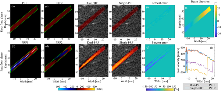
Fig. 8. (Color online) Color Doppler images of the pulsatile flow setting from the transmission angle of  The green box shows the RoI used in the experiment. (a)–(d) Original color Doppler images acquired at each PRF in (a), (c) slow flow phase and (b), (d) fast flow phase. (e), (f) Color Doppler images de-aliased by the dual-PRF method. (g), (h) Color Doppler images de-aliased by the single-PRF method. (i), (j) Relative percent error maps between dual-PRF and single-PRF de-aliased images. (k) The ultrasound beam directions at each pixel. (l) Velocity profiles at the flow channel center of (b), (d), (f), (h) along the white line shown in (b).
Download figure:
Standard image High-resolution image3.1.1. Causes of errors observed with the dual-PRF de-aliasing method
Both the constant and pulsatile flow experiments showed that the dual-PRF approach successfully increased the Nyquist speed of the color Doppler to twice that under the PRF1 condition, and the aliased regions colored in blue in Figs. 7(a) and 8(b) were appropriately corrected as shown in Figs. 7(d) and 8(f), respectively. As shown in Figs. 7(f) and 8(j), the de-aliased flow speed values were comparable to those calculated with the single-PRF approach (manual de-aliasing). However, high errors were found near the wall under the lower left area in both flow conditions, except for the slow flow phase of the pulsatile setting. It is suggested that the error became higher near the wall when the angle between the beam and flow directions became small. The following two factors might be related to those observations: (1) inadequate clutter filtering and (2) high variance in the Doppler signal at the boundary of the aliasing regions. When the clutter filtering was not appropriate (e.g. the filter excessively suppressed the slow flow velocities near the wall in the fast flow phase), the flow speed estimation in the color Doppler was affected and might have been underestimated, as shown in the expanded view of Fig. 7(b). The optimal clutter filtering approach for the proposed framework needs to be investigated in future study, e.g. using an adaptive adjustment of filtering parameters. 31) Moreover, the gradient of the flow speed in the flow tract was observed to increase in the lower left area as the angle between the acoustic beam and low direction decreased. When the original color Doppler images had aliasing artifacts, the spatio-temporal variance in the Doppler signals at those regions also increased and might affect the flow speed estimation. 32) For instance, the color Doppler image measured at PRF2 in the fast flow phase [Fig. 8 (d)] had a region of positive values with one-cycle of aliasing in the lower left area and might have a high-velocity gradient between the wall side and center of the flow tract.
In the dual-PRF de-aliasing approach, the errors in the original color Doppler images could affect the accuracy of the flow speed estimation because the method utilized the differences between the flow speed values measured at different PRFs. As shown in Eq. (4), the difference between two values ( ) was rounded using the
  function and used as
  to determine the aliasing conditions at each pixel. For example, under the settings for this experiment (
 = 310 mm s−1 at PRF1: 2 kHz), the absolute difference between
  and
and  had to be in
  mm s−1 of the expected difference shown in Fig. 1 or it would provide an incorrect
  value. Figure 9(a) shows a map of the
  values for the images in Figs. 8(b) and 8(d). The
  value was properly estimated as 0 in the upper right area, which sequentially turns to −2 and then to 1 along the flow channel center, which corresponded to the observations in Fig. 8(l). However, the estimation of
  value tended to be uncertain in the lower left region and the near-wall region, where
  values were higher than 0.25 [Fig. 9(b)]. This uncertain region agreed with the high-error region, where the relative percent error in Fig. 8(j) is lower than −10% [Fig. 9(c)]. Thus, the dual-PRF approach might produce a spurious flow speed estimate when the original color Doppler has erroneous values. To improve the accuracy and robustness of aliasing-free flow speed estimation in the dual-PRF approach, it might be effective to combine the proposed method with a block matching scheme,
33) referring to the extended least-squares method previously reported.
34)
values were higher than 0.25 [Fig. 9(b)]. This uncertain region agreed with the high-error region, where the relative percent error in Fig. 8(j) is lower than −10% [Fig. 9(c)]. Thus, the dual-PRF approach might produce a spurious flow speed estimate when the original color Doppler has erroneous values. To improve the accuracy and robustness of aliasing-free flow speed estimation in the dual-PRF approach, it might be effective to combine the proposed method with a block matching scheme,
33) referring to the extended least-squares method previously reported.
34)

Fig. 9. (Color online) (a) The  map for color Doppler images of fast flow phase [Figs. 8(b), 8(d)]. (b) The uncertain region
  map, and (c) The uncertain map overlayed on the high-error region [<−10% in Fig. 8(j)]. The red box shows the RoI used in the experiment.
Download figure:
Standard image High-resolution image3.2. Verification of the robust 2D flow vector estimation
Figure 10(a) shows the flow vectors under the constant flow setting visualized using the dual-PRF, dual-angle vector Doppler method. It clearly shows that the method achieved a robust flow vector estimation that successfully corrected the aliasing artifacts, which could be seen as the wrong direction and speed [Fig. 10(b)] when the flow vectors were calculated without any aliasing correction. The flow vectors obtained using the proposed method were comparable to those measured with PIV [the ground-truth in this study; Fig. 10(c)]. In addition, the flow speed profiles measured with the proposed method and PIV are shown in Fig. 11. For each profile, the absolute value of the estimated flow vectors along the short-axis cross section of the flow tract was calculated and plotted. The profile data were generated by averaging the 2D flow vectors over 100 frames and approximately 11 mm along the flow direction from the center of the image. Although the dual-PRF de-aliasing method showed a spatial flow speed profile that was similar to that of the PIV method, the peak flow velocity obtained with dual-PRF, dual-angle vector Doppler was lower (627.4  42.7 mm s−1) than the value of 849.3
  3.9 mm s−1 measured by the PIV method, and the relative error at the flow channel center was −26.1%. The error might have occurred because the flow vector estimations based on the color Doppler imaging and least-squares fitting methods tended to underestimate the peak flow speed as a result of the nature of the mean phase-shift estimations.
19,35)
3.9 mm s−1 measured by the PIV method, and the relative error at the flow channel center was −26.1%. The error might have occurred because the flow vector estimations based on the color Doppler imaging and least-squares fitting methods tended to underestimate the peak flow speed as a result of the nature of the mean phase-shift estimations.
19,35)

Fig. 10. (Color online) 2D flow vectors in the constant flow measurement. (a) dual-PRF, dual-angle vector Doppler method, (b) dual-angle vector Doppler method without aliasing correction, (c) PIV measurement. Note that the flow tract in (a) and (b) is tilted because the ultrasound probe was tilted at  during the measurement.
Download figure:
Standard image High-resolution image
Fig. 11. (Color online) Flow velocity profiles estimated with the proposed and PIV methods across the short-axis cross section in Fig. 10.
Download figure:
Standard image High-resolution imageFurthermore, the flow vectors under the pulsatile flow setting (for both the slow and fast flow phases) measured with the proposed method and PIV are shown in Fig. 12, and their flow speed profiles along the short-axis cross section are shown in Fig. 13. The dual-PRF and dual-angle vector Doppler methods yielded flow velocity profiles similar to those of the PIV method. As also shown in Fig. 11, the estimated peak flow speed (605.9  106.5 mm s−1) obtained with the proposed method was slightly lower than that (708.5
  8.6 mm s−1) obtained with the PIV method in the fast flow phase, while the proposed method showed a slightly higher speed (162.1
  24.6 mm s−1) than that of PIV (119.9
  5.2 mm s−1) in the slow flow phase. The relative percent error at the flow channel center were −14.5% in the fast flow phase and 35.2% in the slow flow phase, respectively. This observation might be related to the spatial and temporal variances of the flow speed, which would have affected the color Doppler measurements.
35)
5.2 mm s−1) in the slow flow phase. The relative percent error at the flow channel center were −14.5% in the fast flow phase and 35.2% in the slow flow phase, respectively. This observation might be related to the spatial and temporal variances of the flow speed, which would have affected the color Doppler measurements.
35)

Fig. 12. (Color online) 2D flow vectors in the pulsatile flow measurement. (a) and (b) show results from dual-PRF, dual-angle vector Doppler method in the slow and fast flow phases, respectively. (c) and (d) show results of the PIV measurements in slow and fast flow phases, respectively.
Download figure:
Standard image High-resolution image
Fig. 13. (Color online) Flow velocity profiles estimated with the proposed and PIV methods at slow and fast flow phases, respectively.
Download figure:
Standard image High-resolution image
Both in the constant and pulsatile conditions, the vector estimation was observed to be unstable especially at the lower left area and near-wall region [Figs. 10(a), 12(b)]. There are two possible reasons on this point: (1) higher color Doppler errors occurred in the de-aliasing process as mentioned in Sect. 3.1.1, and (2) decreased differences between two transmission angles. Due to the nature of dual-angle diverging wave transmission, the difference between the two transmission angles becomes smaller in the deeper region that affects the accuracy of the vector estimation as shown in the previous studies. 19) Moreover, either in the proposed method or PIV, the spatial flow speed profiles (Figs. 11 and 13) were not observed to be parabolic as those expected in the straight tube phantom. This might be caused by multiple factors such as the deformation and surface properties of the flow tract and turbulent flow component as the Reynolds number was approximately 3000. 36) Further evaluation of the accuracy of the proposed method is necessary, such as by precisely synchronizing two measurement modalities that will enable simultaneous acquisition of the target flow profiles.
Finally, with the imaging parameters used in this study, the theoretical extended Nyquist speed was approx. 930 mm s−1 as listed in Table III, which was slightly lower than the peak flow speed (approx. 1000 mm s−1) in the left ventricle. This study only tested the proposed framework with straight tube models, and the maximum flow speed did not reach the extended Nyquist flow speed limit. Also, the present study has not taken into account complex flow patterns such as vortex flow and flow jet that would present in the heart. Therefore, in future studies, the efficacy of the proposed method and the optimal imaging parameters including the combination of p and q in Eq. (2) and the PRFs, should be investigated further in more realistic models, such as a left ventricle model. 37)
4. Conclusions
In this study, we devised a new 2D vector flow imaging framework combined with a dual-PRF de-aliasing method for ultrasound diverging wave imaging with a sector probe. The proposed method showed its merits in the measurement of constant and pulsatile flows and successfully visualized 2D flow vectors without aliasing artifacts.
Acknowledgments
This study was partly supported by the MEXT Leading Initiative for Excellent Young Researchers (LEADER) program, and JSPS KAKENHI Grant Number 20K22968.