Dynamic Microsimulations of Regional Income Inequalities in Germany
- Federal Statistical Office (Destatis), Germany
- ZDF Digital, Germany
- University of Duisburg-Essen, Germany
Abstract
Income is one of the key indicators to measure individual opportunities, regional differences, and societal inequalities. Previous research has shed considerable light on gender- and migration-related disparities at the national level. However, the regional distribution of these inequalities, especially over time, has received less attention. Moreover, how these regional inequalities might develop in the future or under different conditions remains unclear. Regionalized dynamic microsimulations provide a powerful tool to analyze individual, household, as well as local long-term income developments under ‘what-if’ scenarios. This contribution examines the potential regional dynamics in gender and migrant income gaps across the districts in Germany. We extend the data, model, and infrastructure of the MikroSim project with an income module that accounts for migrant groups. By simulating four independent scenarios, we can isolate and evaluate their unique effects on inequality dynamics within different regions. Specifically, we adjust the full-time employment rates and tertiary education levels for a) women to align with those of men, and b) immigrants to align with those of the majority population, separately for each district. The results show that the scenarios have regionally differing effects on inequality dynamics, highlighting the considerable potential of dynamic microsimulations for regional evidence-based policies.
1. Introduction
There is a broad consensus that equal opportunities within the labor force are essential for economic growth, development, and poverty reduction. Women and migrants often experience unequal treatment in the labor market. In addition, migrant women face a ‘double wage penalty’, further increasing their labor market vulnerability (Beyer, 2019). Income and wages provide important foundations for analyzing gender- and migration-related inequalities in measurable outcomes. Previous research has shed considerable light on the gender and immigration wage gaps across countries, while the regional research dimension of these differences has emerged more recently (Fuchs et al., 2021; Schmid, 2022).
In Germany, wage inequality is regionally heterogeneous and characterized by three stylized facts: first, differences between urban and rural areas are significant, like in many other countries. Second, historically grown disparities between the East and the West prevail even 30 years after reunification.1 Third, the labor markets in northern and southern Germany are structurally different. How these wage differences translate into regional pay gaps by gender and immigration remains unclear. In addition, the pay gaps depend to a large extent on the regionally varying characteristics of the local female and migrant labor force. The ratio and composition of ethnic groups differ between the regions in Germany, and the effect of migration background on earnings varies markedly by region (Hillmert, et al., 2017). In urban areas, for instance, the migrant pay gap is found to be higher (Schmid, 2022), whereas the gender pay gap in urban areas is lower than in rural regions (Busch and Holst, 2008). In addition, not only the local values of the pay gaps but also the relative importance of individual and structural characteristics differ drastically across the 401 German districts (Fuchs et al., 2021).
While these studies focus on log hourly wages, monthly net income provides a more comprehensive picture of well-being by taking into account differences in hours worked. Information on regional income inequality in Germany is scarce, and even less is known about its development over time. In Germany, equality of living conditions has constitutional status. Therefore, it is essential for institutions and policymakers to know in which regions inequality is particularly pronounced and to anticipate how these inequalities might evolve in the future to design effective local policies. Hence, this paper focuses on the question of how gender and migration income gaps vary regionally over time, e.g., in terms of urban-rural and East-West differences. The simulation is conducted at the regional level, with income inequality modeled at the district level (NUTS 3) to provide insights into specific regional differences and dynamics.
Increases in the migrant pay gap (Amo-Agyei, 2020) and an only slightly decreasing national gender pay gap over the last decades (Statistisches Bundesamt, 2023b) suggest that neither wage gap is likely to close in the near future. In addition, analyzing long-term income dynamics is important because the driving factors of income changes are entangled across domains, and demographic effects and reinforcement mechanisms may take time to appear (Richiardi and He, 2020). Therefore, how these regional disparities will evolve in the future or under different conditions is of particular interest. Dynamic microsimulation captures the future dynamics of regional income inequalities using ’what-if’ scenarios.
Differences in work- and education-related aspects, such as hours worked, employment status, and educational attainment, explain large parts of the average gender- and migration-related gaps in earnings. Therefore, we adjust the full-time employment rates and tertiary education levels for a) women to align with those of men, and b) immigrants to align with those of the majority population, separately for each district. This paper is based on the data, model, and infrastructure of the MikroSim project (Münnich et al., 2021).2 For our analysis, we have developed an income module for MikroSim that accounts for specific migrant groups and considers relevant individual, household, and regional characteristics.
The present paper is structured as follows: first, we give an overview of the current research on gender and migrant income gaps. Second, we summarize the literature on existing dynamic microsimulation models focusing on income modeling. In the subsequent sections, we present the model and data for our microsimulation and derive the scenarios. Finally, we present and discuss the results according to the different scenarios and conclude with suggestions for further analysis.
2. Income gaps in time and space
Income inequality in a society can be measured by a variety of indicators. We focus on mean income inequality by gender and immigration. The income gap between men and women is an indicator of gender equality in a country, as well as of labor, taxation and childcare policies. The wage gap between immigrants and the majority population is a measure of integration in a society and the adequacy of immigration-related labor market policies. Lower wages of women and immigrants, as captured by gender and migrant pay gaps, pose central issues of our society today that not only exist between countries (OECD, 2017; Amo-Agyei, 2020), but also across smaller geographic areas.
2.1 Gender income gap literature
With a gender pay gap of 18% in 2021, Germany remains among the EU states with the highest gender inequality (ranking 3rd out of 27) (Statistisches Bundesamt, 2023a). The gender imbalances are distributed unequally across space, with local values rangeing from 40.3% to 4.3% on the district level (Fuchs et al., 2021). These profound spatial disparities reflect diverging outcomes in local labor markets for men and women, and thus direly require explanations. While the literature has extensively explored the driving factors of gender gaps across countries and over time, why these gender disparities and pay gaps are context-specific has attracted less attention.
Cross-country and national research has identified a variety of wage-determining characteristics. These include, inter alia, differences in human capital between men and women (Mincer, 1958), work-force interruptions, discrimination, occupational segregation (Busch, 2013), unionization, part-time working, and parenthood (Angelov et al., 2016; Kleven et al., 2019). Over the last decades, there has been a narrowing of the gender difference in education and skills (Doorley and Keane, 2020), whereas employment patterns still vary drastically between men and women.
The existing literature on regional inequality in Germany emphasizes East-West differences. Regarding gender aspects, Hamjediers (2021) provides evidence that gender ideologies diverge regionally due to different compositions and norm persistence across German regions. Liberal gender beliefs are widely spread in the East, whereas an institutionalized traditional male breadwinner model prevails in the West. Regional gender ideologies translate into gendered outcomes through individual behavior and regional institutions, for instance, public childcare provision.
Further studies that explicitly take gender differences in regional wages into account focus on the contrast between rural and urban regions. The gender pay gap is far lower in metropolitan than in rural areas since cities offer increased employment opportunities to highly-qualified women (Busch and Holst, 2008), which are particularly relevant when assuming that partnership ties and family responsibilities impose spatial constraints on women, ‘thereby confining them to the local labor markets of their residential area’ (Nisic, 2017). In addition, more densely populated labor markets are more competitive and restrict employers’ ability to discriminate against women (Hirsch et al., 2013). A further explanation is that agglomeration effects lead to urban wage premium, which is found to be larger for women in the UK (Phimister, 2005) and in Germany (Nisic, 2017).
Beyond the degree of urbanization, a recent study suggests that the economic activity in a region and the kind of jobs provided for gendered earnings are additional important drivers of regional gender pay gaps in Germany (Fuchs et al., 2021). The authors document significant spatial heterogeneity in gross wages at the NUTS 3 level (401 districts) in Germany for the year 2017, which they trace back to spatial variation in individual, firm-level, and regional characteristics. This provides evidence that regions with large firms and a strong manufacturing base, predominantly located in the South of Germany, feature higher gender pay gaps than regions with weaker economic structures.
The majority of the studies focus on the gender pay gap in terms of gross (hourly) wages, which, however, falls short as an indicator of gender inequalities. Even if female and male hourly wages were equal, significant discrepancies in the monthly earnings would persist due to strongly differing employment patterns of men and women. In addition, the wage differentials have consequences on individual career trajectories with implications for equality and poverty both during working life and into retirement, since current wage gaps manifest themselves in the pension gaps of the future (Dekkers et al., 2020). To give a more comprehensive picture of gender gaps in earnings, the gender overall earnings gap (GOEG) measures the impact of the differences in average hourly wages, the monthly average of the number of hours paid, and the employment rate for men and women. With 42% in 2018, Germany is among the EU countries with the highest GOEG (Leythienne and Pérez-Julián, 2021). Another branch in the literature examines gender differences in disposable and market incomes. Two opposing forces act upon the gender income gap. On the one hand, lower employment rates and fewer working hours among women combined with wage disparities widen the gap in overall earnings. On the other hand, the tax-benefit system cushions the gender imbalances in net income by redistributing between men and women (Haupt and Strauß, 2022). According to Doorley and Keane (2020), the main drivers are the disparities in working patterns between men and women – which vary across and within regions.
The question arises, (if and) to what extent gender-specific disparities in income depend on the structure of locally varying employment patterns. To understand inequality in living standards within and between regions in Germany, we examine the spatial component of gender gaps in net incomes. The aim is to investigate regional differences in the distribution of disposable income between men and women and the impact of regional labor supply on these disparities.
2.2 Migrant income gap literature
The migrant labor force plays a signifi cant and growing role in economies of the so-called ‘high-income countries’ (HIC;3 Amo-Agyei, 2020, p. 14). Nevertheless, inequalities between migrants and the majority population persist and have even grown in recent years: the international average of the hourly wage gap is about 13%, with the gap widening in many HICs (Amo-Agyei, 2020). Moreover, the international comparison estimates a ‘double wage penalty’ of nearly 21% for migrant women relative to non-migrant men in most HICs. A large part of the wage gap can be explained by individual characteristics such as human capital, age, and gender. Yet, even if all these measurables are taken into account, significant wage gaps remain in nearly all HICs, pointing to inequalities and potential processes of discrimination against women and migrants in developed economies (Amo-Agyei, 2020).
Recent studies based on the German Socio-Economic Panel data show a similar tendency for the migrant income gap in Germany. Beyer (2019) estimates a raw hourly migrant wage gap of 15.3% in the year 2013, whereas the gap is higher for women (17.9%) than for men (13.3%). In addition, the results point to a severe ‘double wage penalty’ for migrant women in Germany, indicating even more labor market vulnerabilities for this group (Beyer, 2019). Ingwersen and Thomsen (2019) estimate significant and growing migrant wage gaps in Germany over time. They find that the average pay gap from 1994 to 2015 was 13.1% for naturalized immigrants and 14.8% for foreigners, whereas there are substantial differences between income deciles and immigrant groups. For example, while the migrant pay gap grows as income deciles increase, the unexplained part of the gap is higher for the lower-income deciles, indicating systematic wage inequalities in Germany. Furthermore, their results show that some migrant groups in Germany, such as Turks, immigrants from the former Yugoslavia or ethnic German repatriates, are more disadvantaged than Southern European immigrants (Ingwersen and Thomsen, 2019). A further study estimates the monthly wage gap between the majority population and people with a migration background to be around 16.2% in 2018 (Statistisches Bundesamt and Wissenschaftszentrum Berlin Für Sozial-Forschung and Bundesinstitut Für Bevölkerungsforschung, 2021) while also finding severe pay gap differences between migrant groups: ethnic German repatriates and migrants from Southwest Europe earn the highest monthly wages among migrants, whereas Turks, immigrants from the former Yugoslavia, Eastern Europe, and refugees experience more significant median income losses. Thus, in light of the heterogeneous patterns of wage inequality by migrant groups in Germany, a projection of possible future developments in the overall migrant gap should account for these differences.
There is a large body of international and country-specific research on migrant income differences and the potential causes of these differences (see an overview of the German literature in Aldashev et al. (2012). An analysis of migrant pay gaps in four European countries shows that education is an essential driver of income, especially in Germany. Yet, even when controlling for educational attainment differences, the majority population tends to have higher income returns for the same academic level. This return on education varies further between EU and non-EU workers, with the latter having lower returns (Coca Gamito, 2022). Beyer (2019) results lead to a similar conclusion: conditional on education, there is a significant wage gap between migrants and the majority population, with highly skilled migrants facing a devaluation of their skills, resulting in the highest income gaps within the migrant population. These results emphasize the importance of capturing differences in educational attainment as well as actual returns to education in the labor market.
Unlike the research on the individual-level drivers of migrant income gaps, studies on regional differences and regional effects on migrant income trends are scarce (mainly due to small-level data availability; Granato, 2009). Descriptive statistics, however, point to a regional aspect of immigration in Germany. There are considerable regional differences in the proportion of migrants in the total population: in western Germany, almost one in three people has a migrant background, whereas, in eastern Germany (excluding Berlin), this is the case for nearly one in ten people (2021: 30.5 and 9.0 percent respectively). Furthermore, there are significant differences in the ratio of immigrants between urban (2021: 33.8 percent) and rural (2021: 16.5 percent) regions (Statistisches Bundesamt, 2022). In addition, recent district-level studies show that there are tendencies of ethnic clustering in metropolitan areas with higher average incomes and economic potentials, but also higher migrant income gaps in those regions (Schmid, 2022; Hillmert, et al., 2017). Hillmert, et al. (2017) also estimate a regionally varying effect of migrant income gaps. Conditional on individual characteristics, immigrants in eastern Germany seem to be able to reduce or even level out the inequalities in their income outcomes, whereas this is not the case in western Germany (Hillmert, et al., 2017). Thus, for projecting regional income differences and analyzing their dynamics, it seems promising to consider both individual and regional effects as well as compositional differences at the regional level.
3. Literature on dynamic microsimulation
Dynamic microsimulation provides an ability to map the possible inequality dynamics and interactions between the drivers of inequality dynamics. In the following sections, its methodological suitability for this research interest will be explored, as well as previous microsimulations of income.
3.1 Why dynamic microsimulation for income analysis?
Statistical simulation methods are used in the social sciences as analytical instruments to project future population developments and analyze complex social dynamics. The best-known simulation methods in social science research are macrosimulations. Statistical offices mainly use macrosimulation for population forecasts (e.g., demographic change, developments in life-expectancy and care needs, or the future share of the working-age population). The used datasets consist of aggregate data, and the projection of the outcomes of interest relies on cross-tabulations of this contextual data. Yet, according to social science theory, the unfolding of social mechanisms and their development over time takes place on the individual level, whereas societal changes are the aggregated results of these individual developments (Coleman, 1986; Kalter and Kroneberg, 2014). This also applies to all income-related statistics - it is the individuals who receive a monthly salary, get promoted, become unemployed, take parental leave, or retire. Thus, to simulate macro-level income dynamics and developments in inequality, the (causal) explanation can only be sought through the micro-level (such as individuals or households) and be derived based on individual characteristics. The method of microsimulation complies with these requirements (Orcutt, 1957).
Most research that applies microsimulation for analyzing social science questions uses the less resource-demanding static microsimulation models (Holm and Rephann, 2004). Unlike static microsimulations, which can identify the short-term effects of a stimulus (e.g., the impact of a tax reform on different population groups), dynamic microsimulations can consider individuals over their life course. The unique feature of dynamic microsimulations is the data-driven projection of individual life-histories: the characteristics of the individuals are annually updated based on individual transition probabilities (Spielauer, 2011). Actors in the dataset can have children, get older, become employed or unemployed, get married or divorced, or die. These characteristics reflect a life-cycle behavioral model (Holm and Rephann, 2004). The individual-level empirical parameters can be estimated from social science studies with the help of nearly all conventional statistical methods: linear or logistic regression, longitudinal, or dynamic modeling (Post and Van Imhoff, 1998). As we are interested in long-term labor market outcomes, which directly connect with population dynamics, we use the approach of dynamic microsimulation modeling.
In addition, the research focus in this article is the modeling of individual income trends in Germany from a regionalized perspective. As Holm and Rephann (2004) point out, the spatial dimension in microsimulations: ‘[…] is a useful addition when (1) it improves the accuracy of microsimulation models by introducing spatial and geographical variables as driving forces of change and (2) it allows results to be presented and interpreted for space and regions.’ (Holm and Rephann, 2004, p. 389). As those aspects are of particular importance in the case of projecting income inequality, we will use the constructed regional base data and dynamic microsimulation modeling in our further analysis. The inclusion of the spatial perspective in the simulation process allows us to choose between different groupings of the analyzed individuals to present results at different higher levels (district, state, east/west, urban/rural, or national). Thus, through dynamic regional microsimulation, we can compare the outcomes in income between the regions in the same year. Additionally, we can focus on one geographical area over time, disaggregating the income development, e.g., by the immigration history or mean educational level. In addition to regional differences, we can take demographic changes in the composition of the population into account. This makes it possible to examine the interplay of causal individual-level mechanisms with compositional and contextual effects on the development of income inequalities.
Furthermore, microsimulation serves as a tool for experimenting, not for exact predictions. Microsimulation can be seen as a ‘scientific computer game’ (Spielauer, 2011, p. 11) to test and compare the consequences of so-called ‘what-if’ scenarios. Questions as to how the world would look under different conditions can be explored. In a regionalized microsimulation, the unfolding of such fictitious scenarios can be played through on the individual level, on the contextual level, or they can emerge exogenously, e.g., through political interventions. Spatial microsimulation is an appropriate technique to build regional profiles, to identify and compare regional patterns of inequality and poverty, which may then lead to ‘improvements in the design of policies tailored to local conditions’ (O’Donoghue, 2021).
3.2 Income models in previous dynamic microsimulations
Researchers use different theoretical concepts and statistical techniques to select and estimate the updating parameters in microsimulation models. Due to the heterogeneity of modeling techniques, complexity in the models, and the long-term characteristic of dynamic microsimulations, microsimulation models are inevitably different and often criticized as ‘black boxes’ (Dekkers, 2014; Spielauer, 2011). Nevertheless, all the models have a common denominator: they try to estimate the individuals and the change in their characteristics with the highest possible overlap with the real world. stress that a poor approximation of the true model in one of the microsimulation modules can induce severe errors and diminish the utility and usability of the whole microsimulation model.
Table A1 gives an overview of microsimulation models that incorporate regression-based income models for future analysis in their dynamic microsimulations. It is not an exhaustive list of all such models in the world, but rather an attempt to shed light on the ‘black boxes’ of relevant and ongoing microsimulation models. We systematize concepts from previous models to compare possible approaches and learn from the best practices for estimating individual employment income in dynamic microsimulations.4
When estimating income, the challenge of finding an appropriate statistical model is exceptionally high. On the one hand, it is demanding to adequately simulate the high heterogeneity between different individuals according to their characteristics as well as within a person’s life cycle (Andreassen et al., 2020). On the other hand, there is state dependency in income projections, i.e., a person’s income in the previous time point affects this person’s income in the next time point.5 Table A1 indicates that almost all of the selected regression style income models capture state dependency in income modeling. The majority of the selected microsimulation models use random effects regression (MOSART; Pensim2, Dynasim 3; SESIM 3; MIDAS Italy and MIDAS Germany; T-DYMM; CBOLT). While only two models each apply OLS (ZEWDMM; MIDAS Belgium) or OLS-LDV (SVERIGE; Bönke et al., 2020), the use of more complex hybrid or dynamic panel models is absent.
Regarding variable selection, all models include the individual characteristics that are at the core of Mincer’s (1974) equation. Depending on the specific modeling purpose, some microsimulation models add a life course perspective on income by measuring the stability of career paths (MOSART) or recent employment experience (SAGE), whilst others concentrate on firm-level characteristics such as firm size (MIDAS) or occupational sector (SESIM 3). DYNASIM 3, one of the many extensions of Orcutt’s (1961) first core dynamic micrsimulation, contains one of the most detailed behavioral income modules with numerous theoretically well-founded individual-level variables (listed in Table A1) and separate estimations for homogeneous response groups by age, gender, and race. Taking the individual immigration history into account is rare in microsimulations. Apart from the DYNASIM 3, three further exceptions are SESIM 3, which controls for nationality, the SVERIGE model, which includes country of birth in its estimation, and T-DYMM, which differentiates between areas of birth (Italy, EU and non-EU). In addition to individual characteristics, most of the selected microsimulations include household variables, such as the number of children or marital status. As emphasized by Holm and Rephann (2004), the possibility to capture behavioral effects, such as demographic and household processes, is a great advantage of microsimulation modeling.
The aim of this paper is to analyze regional gender- and migration-related differences in income. Regional aspects of income modeling have hardly been taken into account in previous models (see Table A1). Only two of the models capture the region of residence (DYNASIM 3) or the regional unemployment rate (SVERIGE) in their income estimates, whereas both also use the regional unemployment rate in their modeling of the individual employment probability.
German dynamic microsimulations have enjoyed rather reserved attention in international research, as the models are relatively small or concentrate on one specific theme (Schnell and Handke, 2020) or cohort. Two promising approaches have increased the visibility of German models in the microsimulation landscape: ZEWDMM microsimulation (see Table A1) is a cohort model and combines tax-benefit simulations with life-cycle modeling to estimate counterfactuals. Another cohort microsimulation in the German context (Bönke et al., 2020) prognoses one’s lifetime labor income according to family and educational status. However, both models focus on one selected cohort and do not cover information on migration or regional details. Overall, Germany lacks a nationwide microsimulation infrastructure similar to the Pensim2 population model or the SVERIGE spatial model, which would operate and enable regional inequality microsimulations in the long term (Schnell and Handke, 2020). This gap is now being filled by the MikroSim project.
4. Empirical strategy
The following dynamic microsimulations are based on the simulation infrastructure of the MikroSim project, which is presented in section 4.1. We enhance the MikroSim model with an income module. Part 4.2 gives details about estimating initial incomes in our base dataset and forecasting incomes during the simulation.
4.1 The MikroSim project
MikroSim is a regional dynamic microsimulation model for Germany (see for a detailed description: Münnich et al., 2021). It is a discrete-time population model with a synthetic dataset based on information from census, administrative, survey, and other small-area datasets. The base population of MikroSim consists of over 80 million individuals and nearly 40 million households modeled within the 401 German districts (NUTS 3). All processes are simulated separately for each district. Mobility between districts is taken into account.6
MikroSim models regional differentiation as well as rural-urban disparities by using appropriate auxiliary variables as regional benchmarks and within the models (Münnich et al., 2021). Starting from the base year 2011, the characteristics of the micro-units are updated deterministically or stochastically based on individual empirical transition probabilities and Monte-Carlo simulation. These updating decisions take place modularly, whereas individuals run through the modules each year sequentially for an adjustable simulation horizon (see Figure 1). Accordingly, MikroSim enables the estimation of regionalized long-term projections of societal dynamics evolving from individual processes and interrelations within the microsimulation population. We use the MikroSim version 2.1.4. (Alsaloum et al., 2022) for our analysis.

Modules in MikroSim 2.1.4. Source: own illustration.
MikroSim currently consists of 15 modules specified in Figure 1, with new modules such as housing, transport choice, and healthcare to follow near-term. In 10 modules, alignment methods are applied to harmonize the simulation outcome with known regional totals.7 We choose a simulation horizon of 30 years. The benchmarks for the open regional mobility module are selected as the median of the last decade’s observed mobility figures.
The income module assigns and projects individual incomes to all employed persons in the labor force (ages 15-64), which will determine the subgroup of our analysis. Nearly all modules in MikroSim are essential in estimating individual income (see Part 4.2), as they either influence the probability of employment and thus the possibility of earning an income or influence income directly via individual income-relevant characteristics.
4.2 Income modeling and forecasting in MikroSim
The income module estimates average monthly individual net income for the working population. Income is defined as the sum of all income components after taxes and transfers, including income from labor, capital, pensions, public payments and other incomes. As explained in Section 2, we believe that monthly net income provides the best picture of what an individual actually has left to spend at the end of the month. First of all, the realized net earnings determine women’s and migrant’s participation in the economy. Moreover, monthly net income captures imbalances in employment patterns which gross hourly wages fail to account for (Leythienne and Pérez-Julián, 2021).
The income models are based on data from the 2011 to 2014 German microcensus. The microcensus provides individual net incomes, i.e. the sum of all income components after taxes and transfers, originally reported in 24 disjunctive classes and interpolated using generalized Pareto interpolation to derive a continuous measure. For descriptive statistics of the interpolated income measure, see Table A5 in the Appendix. The estimation comprises two steps: (1) the assignment of initial earnings in the beginning of the simulation and throughout the simulation for each individual that enters the labor market and (2) the projection of incomes for individuals who have already been employed in the previous period. As described in Section 3.2 and shown in Table A1, a similar procedure is chosen by Holm et al. (2007).
Initial earnings are estimated for the working population before the start of the simulation and for each individual that enters the labor market during the simulation based on Equation 1. The majority of dynamic microsimulation models reviewed in Section 3.2 use random effect modeling approaches.8 Following this consensus, we estimate a model of the following form for initial earnings:
with being the individual net incomes, the observed characteristics, the coefficients, and the normally distributed error terms for each individual at time . The independent individual random effects capture unobserved heterogeneity. The covariates cover individual, household and regional aspects whereas the latter also serve as a proxy for regional employer characteristics (see Table A2 in the Appendix).
The simulation of initial income is based on the attributes and the estimated associated parameters from Equation 1, which are presented in Table A3, and the disturbance term . The latter is drawn from a normal distribution with estimated variance and added to the mean income predictions for each individual. Moreover, the individual random effect from Equation 1 is added once at the start of the simulation and used for predictions over the whole life cycle representing the individual’s ability.
In the course of the simulation, the projection of earnings is modelled by:
with independent individual random effects capturing unobserved heterogeneity and lagged incomes . For the projection of income for those who have been in the labor market in the previous period, we use the estimated coefficients from Equation 2, shown in Table A4 and draw a disturbance term from a normal distribution with estimated variance from Equation 2 and add it the mean predictions.
In general, aligning income modules can enhance the accuracy and policy relevance of the models by capturing income disparities more realistically. In other words, alignment ensures the consistency of the disaggregated inequality measures with known macro figures. However, the alignment also comes with challenges related to the data limitations, oversimplification, model complexity, and the potential of manipulation. In the case of MikroSim, the income module was not aligned due to the absence of adequate regional benchmarks, conceptual differences in available income measures, and to avoid further assumptions. Furthermore, if the survey income distribution and chosen benchmarks significantly differ and no data for distributional adjustments are available to make the two sources consistent, aligning the income module to income aggregates results in a change in income distribution. As a result, O’Donoghue et al. (2013) chose not to calibrate average incomes in their microsimulation model to national accounts totals. In addition, most of the microsimulation models reviewed in Table A1 and Section 3.2 do not calibrate income to known benchmarks. Alignment of income to growth assumptions or other projections is more commonly utilized in various models such as DYNASIM 3, MIDAS, T-DYMM, and CBOLT. DYNASIM 3 employs wage growth assumptions for future periods, MIDAS uses corrected growth rates and macroeconomic productivity assumptions, T-DYMM incorporates labor productivity growth and consumer price index, while CBOLT utilizes economic projections. In addition, a linkage of our MikroSim model with a macro model including labor demand is currently being tested. However, it is not essential for the answering of the research questions of this paper.9
We estimate the models separately for men and women.10 The separate modeling for female and male workers follows the suggestion of Blinder (1973) and Oaxaca (1973). In addition, as explained in Table A1 most other microsimulation models also differentiate their models by gender. Figure A3 in the Appendix presents maps of the relative spatial income distributions from our simulated MikroSim income compared to data from the Tax Statistics and the Federal Employment Agency. For all three datasets, the spatial distribution is relatively similar, with male income largely driving overall regional disparities.
4.3 Driving factors of income gaps & ‘what-if’ scenarios
After modeling income and incorporating it into the microsimulation, we shift to analyzing gender and migration inequalities in income gaps. We apply the Blinder-Oaxaca decomposition method (Blinder, 1973; Oaxaca, 1973) by using the R package oaxaca (Hlavac, 2022) to analyze mean income differences in the working population across gender and immigration status. These analyses aim to determine what proportion of the gap is due to compositional differences in the characteristics of individuals and to what extent the effects of the influencing variables differ systematically depending on the group studied. To analyze the possible dynamics in the gender and migrant gaps, we must understand the driving forces and the differences in the composition of the population according to income-relevant factors. Hence, the following empirical results provide a better understanding of the future dynamics and the rationale for our ‘what-if’ scenarios.
In our analysis sample, the average net income of men is about 2300 euros, while women have about 1400 euros per month at their disposal. The resulting difference can be attributed to variations in the magnitude of the effects between men and women of approx. 55%, to group allocation differences of approx. 30% and to their interaction of approx. 15%.11
The decomposition results show compositional differences between the sexes in part-time, higher education, white-collar workers, and self-employment (see Figure A1, Endowments). Of these, the strongest driver of the gender pay gap is the difference in the share of part-time employment between women and men (47% vs. 9%). More men are self-employed, which enlarges the gap, yet a higher proportion of women fill the white-collar jobs, which reduces the gap as these jobs are better remunerated. Furthermore, slightly more men than women (30% vs. 25%) have a university degree - a former trend that has already reversed in the younger cohorts and will become visible in the overall composition of the population in the long run (OECD, 2022).
In addition, the magnitude of the coefficients of some variables differs according to gender (see Figure A1, Coefficients). For example, the effect of being married is 480 euros larger for men than for women, i.e., men seem to gain from being married (390 euros), while women seem to even lose on average (90 euros). The same applies to the income effect of a university degree, which is, on average, 300 euros higher for men than for women, indicating that the utility of tertiary education is in favor of men. Although women suffer less income loss from working part-time compared to men, this cannot compensate for the large gap in working hours described above.
Based on the decomposition results, we want to explore the overall gender income gap developments in a scenario where there are no differences in the composition of part- and full-time work between the sexes. Given that the share of women working part-time is nearly 38 percentage points higher than that of men, this is the most crucial factor for the unadjusted income gap in Germany and therefore serves as the first scenario in our microsimulation. In this context, it is particularly interesting to see how the effects of the scenario differ regionally, as the starting points of full-time female employment within Germany are historically different. Scenario 1: how much would the regional gender gaps in income reduce if women’s working time was equal to that of men?
In the second scenario, we are interested in the contribution of differences in the educational attainment between the sexes on the development of the gender income gap. The results in Figure A1 show that the higher share of men with tertiary education widens the gender income gap. Moreover, as the gender ratio in tertiary education is changing in favor of women, the possible outcomes can only be analyzed from a long-term perspective. That leads us to our scenario on egalitarian endowments of higher education: Scenario 2: how would the dynamics of the gender income gap develop if the share of tertiary education was the same for women as for men?
The average net income of the majority population (women and men) in our study sample lies at around 1900 euros, while the average income of migrants is around 1600 euros per month. Thus, the unadjusted migrant income gap amounts to about 15%.
Systematic compositional differences between migrants and the majority population are found in nearly all variables in the model. The driving forces that widen the gap (see Figure A2, Endowments) are the higher proportion of migrants with lower educational attainment (9% vs. 28%) and, in contrast, the lower proportion of migrants with tertiary education (29% vs. 22%). In addition, the majority population is more frequently employed in government and white-collar jobs than the migrant population, while migrants are more likely to work part-time, further widening the income gap. Compositional effects that narrow the gap include the group-specific allocation in regional variables. Migrants are more likely to be located in areas with higher population density and in western and southern Germany, whereas fewer migrants reside in areas with higher unemployment rates and in eastern and northern Germany. This suggests that allocation dynamics play an essential role in moderating migrants’ future incomes, which must be considered when projecting inequalities between the migrant and majority population.
Furthermore, the decomposition results show group differences in some of the coefficients (see Figure A2, Coefficients). Compared to post-secondary education, the income losses of the majority population due to lower education are even more severe than for the migrant population. For tertiary education, however, the benefit for the migrant population is, on average, 71 euros lower than for the majority population. The income loss from working part-time is in turn higher for the majority population as for the migrant population, narrowing the migrant income gap on average. Yet, it can not counterbalance the gap-widening compositional effects of more migrants in part-time employment discussed above.
Based on the decomposition of the migrant income gap, we are interested in manipulating one of the main explanations behind the differences – the share of full-time employment in the migrant population. Our scenario will level out the differences of 19 percentage points in working time, thus ‘assimilating’ the working hours of the migrant population with the working hours of the majority population. It is interesting to see the possible effects of this adjustment, as the magnitude effects discussed above have shown that the increase in income from part- to full-time employment is not as strong for migrants as for the majority population. Scenario 3: how much would the income gap between migrants and the majority population be reduced if migrants’ working hours were equal to those of the majority population?
The second scenario regarding the migrant income gap addresses educational differences in tertiary education. As seen in the compositional effects, the lower share of migrants with a university degree widens the income gap between migrants and the majority population. Thus, leveling this compositional effect of tertiary education gives a better picture of the inequality-reducing potential in educational integration processes. Moreover, the regional perspective is relevant here because the proportion of migrants with tertiary education shifts as migrant groups change (Granato, 2014), and, the allocation and composition of those changing migrant groups diverge regionally. Scenario 4: how would the regional dynamics of the migrant income gap develop if the share of tertiary education were the same in the migrant population?
All our scenarios start in 2020 when the calibration of our simulation currently ends. The scenarios are implemented by adjusting the regional relative benchmarks for full-time employment and higher education for women and migrants to match those for men and the majority population, respectively. We chose to model these scenarios with the intention of explaining the maximum possible reduction in income inequality that can be achieved if the scenario under consideration applies.
5. Microsimulation results
This section describes the effects of the four scenarios on the regional gender and migrant income gaps over time. Our results indicate that the gender income gap in Germany starts at roughly 38% in the base year 2011 and narrows to 26% over the course of the 30-year simulation horizon. In contrast, the migrant income gap is 13% in 2011 and remains at about the same level over 30 years. Our initial values are in the same range as other statistical estimates, although no fully comparable benchmarks exist (see Chapter 2).
5.1 Baseline results
Figure 2 shows the development of mean income values from 2011 to 2040. By 2020, income is increased due to the upward calibration of other modules that affect income estimation. Structural increases in the covariates lead to increases in the estimated mean incomes, such as rising numbers of births in the first five years of the simulation (which are aligned with observed regional benchmarks) and higher levels of tertiary education. Average income gains are slightly higher in eastern Germany, so there is a modest convergence between east and west in urban and rural areas. From 2020, we see a convergence in mean incomes between urban and rural areas in the West (note the green lines) and a divergence in the East (note the blue lines).
In addition, Figures A4–A6 in the Appendix show the simulated working, total, and migrant population by regions and degrees of urbanization. Overall, the simulated labor force and population figures are relatively stable over time. In the East, the simulated population shows tendencies of rural exodus. Population aging is particularly pronounced in the West: While the simulated labor force declines from 2020, the total simulated population of western Germany remains relatively constant. Furthermore, over the entire simulation period, a constant trend in immigration inflows is projected. Notably, the cumulative number of first-generation migrants is rising, particularly in western Germany and urban areas. Understanding the evolution of these regional demographic trends holds significant relevance for income estimation. Urbanization, for instance, contributes to the increase in average incomes; however, it has divergent effects on gender and migrant income gaps (see Section 2). For an overview of the development of all the explanatory variables between 2011 and 2040, see Table A6 in the Appendix.

Mean income by region in the base scenario.. Note: The figure shows the simulated mean income values from 2011 to 2040. The colors indicate regions: East Germany (blue) and West Germany (green). Source: own illustration.
5.2 Gender income gap results
To shed light on the regional scenario effects over time, Figure 3 compares the dynamics of the gender income gap in the East (blue) and West (green). Our results indicate gender income gaps of roughly 17% in the East and 33% in the West of Germany in the year 2020, which is in line with the current literature. For instance, Bönke et al. (2020) and Fuchs et al. (2021) also find larger gender gaps in western Germany. Regarding dynamics, there are three key findings: first, the gender income gaps are closing over time in the baseline scenario. Second, the decrease is more pronounced in the East. Third, both scenarios accelerate the narrowing; especially the full-time scenario.
One aspect that contributes to the differences in dynamics between East and West Germany is the heterogeneity of male incomes, which are unaltered across all scenarios. On average, men are paid less and there are fewer top earners in eastern Germany than in the West, and female incomes are more homogeneous across Germany. The gender income gap in the East is primarily due to lower earnings of women, while in the West, it is driven by higher incomes of men (see Figure A3 in the Appendix). This means that women’s earnings contribute disproportionately to the gender income gap in the East. As women’s earnings increase, the income gap is closing faster in the East compared to the West. Fuchs et al. (2021) also find that gender differences in individual characteristics are important drivers in regions with low gender pay gaps, while job-related characteristics are more relevant in regions with higher gaps.
Several factors drive the reduction in the simulated gender income gap in the baseline scenario. First, the decline in marriages, the emergence of new living arrangemkents, and the decline in birth rates strongly impact the income distribution. Second, women’s rising educational attainment levels between 2011 and 2040 improve their access to higher-paying job opportunities (see Figure A7). Additionally, women moving to urban areas and benefiting from the urban wage premium narrow the income gap (as illustrated in Section 2.1).12 Lastly, the increasing presence of women in state-worker and white-collar occupations, which offer higher salaries, also contributes to reducing the dynamics of the gender income gap (see Table A4 for the coefficients, Table A6 for the development, and Figure A1 for the relative importance of the factors).

Gender income gaps by region and scenario.. Note: The figure shows the simulated percentage changes in the gender income gap from 2020 to 2040. The colors indicate regions: East Germany (blue) and West Germany (green), while the line types differentiate between the scenarios: base (solid), university endowments of women adapted men (dotted), and full-time rates women adapted to men (dashed). Source: own illustration.
Figure 4 disentangles the dynamics between rural and urban regions by extending the previous comparison with the additional district type dimension. The left and right side show results for rural and urban districts respectively. The differences between rural and urban areas are relatively small in the West, whereas a rural-urban divergence is observed in the East. Urban regions are associated with a large reduction in the gender income gap in the East, which is most pronounced in the full-time scenario. Hence, the fact that working-age women in East Germany live mostly in urban areas accelerates the closing of the income gap in the East, especially in the full-time scenario.

Gender income gaps in East and West by district type and scenario.. Note: The figure shows the simulated percentage changes in the gender income gap from 2020 to 2040 for rural (left side) and urban areas (right side). The colors indicate regions: East Germany (blue) and West Germany (green), while the line types differentiate between the scenarios: base (solid), university endowments of women adapted men (dotted), and full-time rates women adapted to men (dashed). Source: own illustration.
Another possible reason for the faster decrease in the East could be less structural discrimination. Especially in urban areas, the potential to discriminate against women is restricted due to more competitive labor markets (Hirsch et al., 2013). In addition, agglomeration effects lead to an urban wage premium, which is found to be larger for women in Germany (Nisic, 2017). In the East, it is more profitable for women to live in urban areas than in rural regions. The difference between eastern and western rural areas can be explained by the fact that many rural areas in eastern Germany are structurally weak, with fewer large and industrial firms, while some rural areas in western Germany have large, well-performing firms in high-paying sectors such as technology and innovation.
For detailed spatial analysis, Figure 5 shows the simulation results at the level of the 401 German districts for the final simulation year 2040, using the baseline (left), Scenario 1 (middle), and Scenario 2 (right). The colors correspond to the size of the gender income gap, with darker colors indicating larger values. All three maps reflect a clear east-west divide. While the largest gender income gaps are observed in the southern and western parts of Germany, the values are much lower in the East.13 Additionally, the urban areas have significantly lower values than the rural regions. Regarding the scenarios, the map of equal full-time rates is much brighter, reflecting the strong reduction in the local gender income gaps with rates between –12 and 26% (compared to the baseline with rates between 1 and 38% and the university education scenario between 2 and 37%). In addition, some negative rates stand out in those regions where women would earn more than men. Our results are in line with Fuchs et al. (2021), who also find local gender pay gaps between –4 and 40% for the German districts.
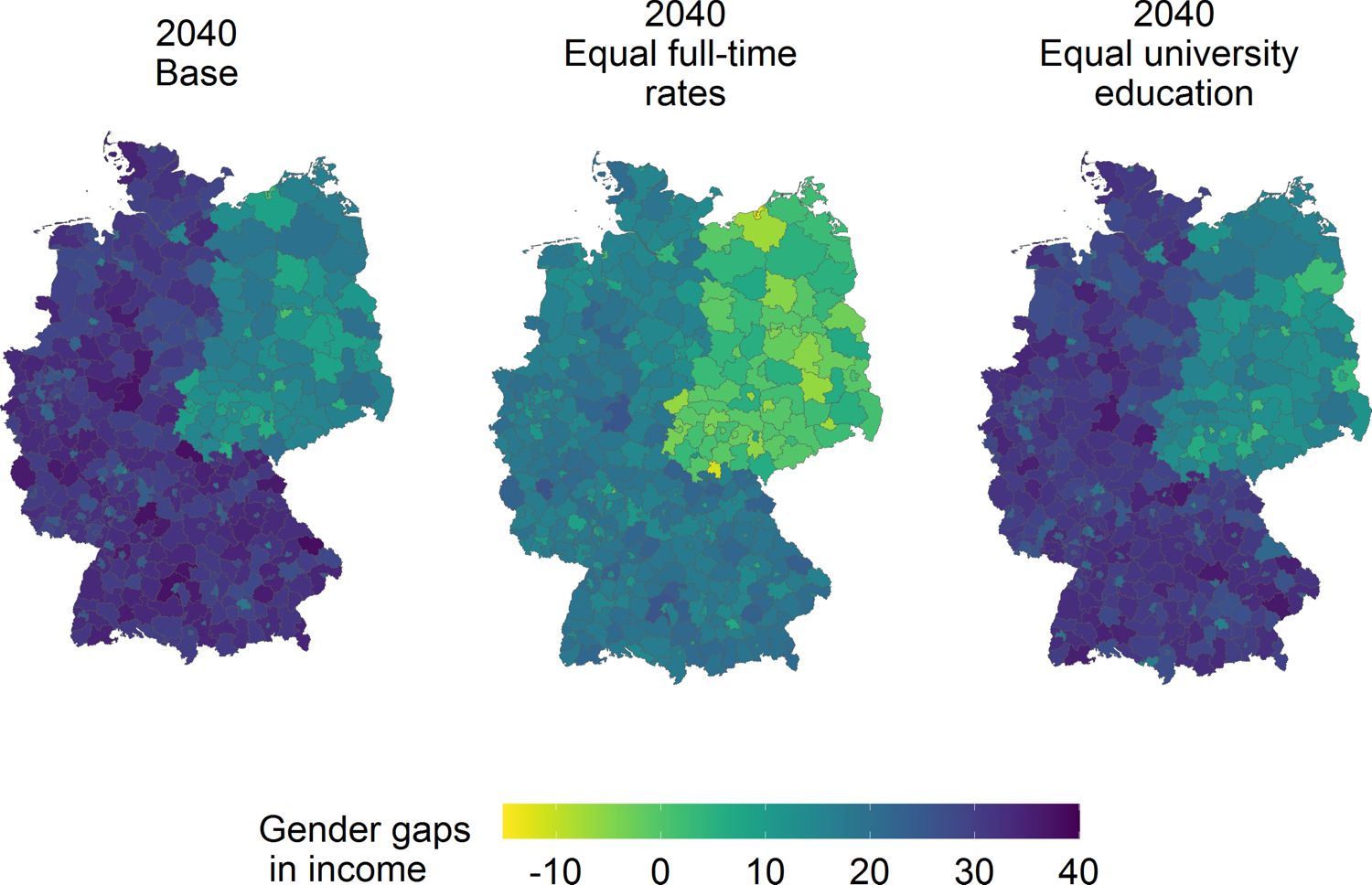
Regional differences in gender income gaps.. Note: The figures illustrate the simulated gender income gaps in 2040 across the 401 German districts under different scenarios: base (left), full-time rates of women adapted to men (middle), and university endowments of women adapted to men (right). Lighter col-ors represent smaller gaps, whereas darker colors correspond to larger wage gaps. Source: own illustration.
In conclusion, these findings suggest that individual work-related characteristics contribute substantially to the gender income gap in the East, while more structural factors, such as job availability and choice, dominate in the West of Germany. Hence, setting the right incentives and socio-economic conditions to change individual behavior, especially in terms of increased working hours, seems to be a promising approach to reduce gender income inequalities in East Germany. In the West, however, more structural changes seem to be essential, such as counteracting occupational and educational segregation or increasing the number of female leaders or top earners.
To reduce the income gap, concrete measures to increase women’s hours worked and educational attainment in Germany include expanding affordable childcare options (Zucco and Lott, 2021). Moreover, companies could be encouraged to implement flexible work arrangements (Boll et al., 2022) and to provide more wage transparency (Peichl and Rude, 2022; Gust and Kinne, 2022). Further promising political measures include expanding quota regulation in gainful employment and care work (Görges, 2022), providing career support programs for women, and offering support for female entrepreneurship (Herold et al., 2022). Another measure tailored to the German context is the reform of the current tax system, specifically concerning ’Ehegattensplitting’ (Peichl and Rude, 2022; Zucco and Lott, 2021).14
5.3 Migrant income gap results
Our simulations estimate a migrant income gap for first-generation migrants who immigrated to Germany themselves. The migrant income gap is relatively stable over the simulation period, while it varies considerably by migrant groups. We find an inverted U-shaped migrant income gap: with a baseline of 13% in 2011 and a peak of 15% in 2019, the gap gradually decreases and is back to around 13% in 2040. This temporal dynamic in the migrant income gap goes hand in hand with the composition of migrant groups: the share of resettlers with relatively high incomes decreases, which increases the gap. In later years, however, the proportion of EU migrants with higher average incomes rises, which narrows and stabilizes the gap. The results are consistent with the heterogeneous income patterns of migrant groups in Germany known from previous studies (Statistisches Bundesamt and Wissenschaftszentrum Berlin Für Sozial-Forschung and Bundesinstitut Für Bevölkerungsforschung, 2021) and underline the importance of compositional dynamics for interpreting simulation results (see Table A6). Furthermore, in the baseline scenario, the educational level of migrants is seen to increase in tandem with the educational level of the majority population (see Figure A8). This progressive trend enables migrants’ incomes to maintain pace with those of the majority population.
Figure 6 shows these dynamics in the migrant income gap differentiated by East (blue) and West (green) Germany. While the migrant earnings gap decreases in both regions from 2020 onward in the baseline scenario, the decline is more substantial in the East and levels out the initial higher earnings gap in eastern Germany. In addition, both scenarios reduce the earnings gap of migrants, with the effect of the full-time scenario showing a steeper decline in the West.
Figure 7 adds another angle on the regional view of the income inequalities between migrants and the majority population according to their residence. It is only in this further regional analysis by rural (left) and urban (right) areas that the scenarios unfold their different spatial implications. The steeper decline under the full-time scenario in West Germany shows an even higher reduction of the migrant income gap in the rural areas of West Germany compared to rural areas in the East. Moreover, equal higher education has only a marginal effect in urban areas, while in rural areas, the scenario has a more noticeable reductive effect on the migrant income gap.
Overall, it can be said that Scenario 3 has the potential, via composition effects, to reduce the migrant income gap by even more than half, especially in the West and in rural areas where more migrants work part-time. Although overall migrant income inequality is somewhat higher in urban areas, the compositional adjustment in Scenario 4 has a lower effect on these areas. This is consistent with previous research on wage differentials, which finds the highest wage differentials in urban areas (Schmid, 2022) and among highly skilled migrants (Beyer, 2019), further indicating a different utility function of education for migrants and the majority population. Thus, the dynamics of the migrant wage gap cannot be reduced universally by simply adjusting composition characteristics, suggesting that a change in individual factors may have an impact in some (here: rural) regions, while in others, job-related characteristics are additionally crucial.

Migrant income gaps by region and scenario.. Note: The figure shows the simulated percentage changes in the migrant income gap from 2020 to 2040. The colors indicate regions: East Germany (blue) and West Germany (green), while the line types differentiate between the scenarios: base (solid), university endowments of migrants adapted to the majority population (dotted), and full-time rates of migrants adapted to the majority population (dashed). Source: own illustration.

Migrant income gaps in East and West by district type and scenario.. Note: The figure shows the simulated percentage changes in the migrant income gap from 2020 to 2040 for rural (left side) and urban areas (right side). The colors indicate regions: East Germany (blue) and West Germany (green), while the line types differentiate between the scenarios: base (solid), university endowments of migrants adapted to the majority population (dotted), and full-time rates of migrants adapted to the majority population (dashed). Source: own illustration.
Figure 8 provides a detailed regional overview of migrants’ income gaps at the end of our simulation horizon by districts in Germany. On the left, we can see the income gaps in the baseline. In the middle, we observe the proportion of migrants in full-time employment (Scenario 3), and on the right, the composition of migrants with higher educational attainment (Scenario 4), aligned with the majority population. The dark-colored extreme outliers on all maps reflect some regions in the East and rural areas with smaller migrant populations (Statistisches Bundesamt, 2022) and should therefore be interpreted with caution. The lighter coloring of the scenario maps indicates that both scenarios show an effect, but only the full-time scenario can substantially reduce the migrant income gap. In contrast to the gender income gap (Figure 5), we do not see a clear east-west division in the migrant income gap.
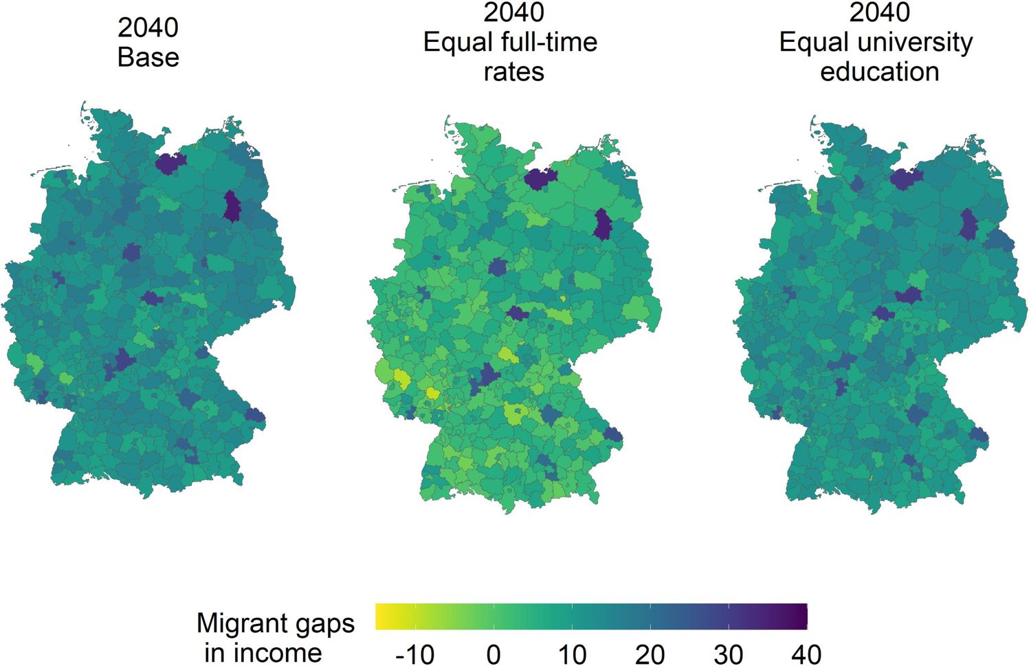
Regional differences in migrant income gaps.. Note: The figures illustrate the simulated migrant income gaps in 2040 across the 401 German districts under different scenarios: base (left), full-time rates of migrants adapted to the majority population (middle), and university endowments of migrants adapted to the majority population (right). Lighter colors represent smaller gaps, whereas darker colors correspond to larger wage gaps. Extreme outliers result from a limited number of observations in some districts. Source: own illustration.
The simulation results are consistent with those of Hillmert, et al. (2017), who estimate regionally varying migrant gaps. However, we find no possibility of leveling out the migrant gaps in the eastern or western regions by controlling for individual characteristics, at least not merely working hours or higher education. As Amo-Agyei (2020) points out, closing the migrant wage gap requires policies that target different levels of income distribution and specific sectors of the economy. Furthermore, counteracting the existing lower returns of higher education could serve as a potential approach for reducing the regional migrant income gap (Beyer, 2019). In this regard, microsimulation shows that it may be beneficial to consider regional characteristics when planning and implementing potential policies to reduce migrant income inequality.
Implementing measures aimed at reducing the income gap between men and women can positively impact the income disparity among migrants as well (see Section 5.2). For migrant women, who often face a ’double wage penalty,’ initiatives such as increasing the availability of childcare facilities, offering flexible work arrangements, and providing career planning support can be particularly beneficial. Migrants also encounter challenges due to the limited transferability of their qualifications, which can hinder their employment prospects and earning potential, especially in Germany (Aldashev et al., 2012). To address this, improving the recognition and applicability of foreign qualifications is essential, enabling individuals to make informed career decisions based on their actual qualifications. This would unlock the full potential of the migrant workforce and reduce economic inefficiencies (Ingwersen and Thomsen, 2019, p. 20). Moreover, migrants have a proportionally higher share of lower educational attainment, as depicted in Figure A2, and often experience ’sticky floors’ in terms of lower wages (Schmid, 2022). Therefore, implementing targeted programs such as vocational training, language and literacy programs, and lifelong learning (Coca Gamito, 2022) can play a significant role in reducing the income gap for migrants. Moreover, in urban areas, where diverging reduction potential in migrant pay gaps is observed (see Figure 7), promoting pay transparency and strengthening anti-discrimination laws can help overcome the ’glass ceiling’ faced by highly skilled migrants (Schmid, 2022).
6. Conclusion
The research literature has extensively examined gender- and migration-related inequalities at the global and national levels, while less is known about the regional dimensions of these inequalities, particularly over time. Although the German government has been striving for equal living conditions, regional disparities persist, particularly regarding regional income differences (Immel and Peichl, 2020). This paper aims to examine the potential dynamics in gender and migrant income gaps across German districts.
We use regionalized dynamic microsimulations to analyze how income inequalities might develop in the long run and under different conditions. The dynamic microsimulation approach allows the modeling of interrelated factors driving the gaps at the individual, household, and regional levels and to capture changes in these characteristics over time. Using the MikroSim model for Germany, we simulate four scenarios adjusting full-time employment rates and tertiary education levels for a) women to align with those of men, and b) immigrants to align with those of the majority population, separately for each district.
The results show that the scenarios affect the regional inequality dynamics differently. Regarding gender inequalities, the future income gaps narrow in all regions, with the largest declines in urban areas in the East and the full-time scenario. The regional migrant income gaps also decrease significantly in the full-time scenario relative to the baseline, whereas here, the declines are more pronounced for rural areas and in western Germany. Hence, increased working hours of women and migrants, which is often discussed as a potential remedy to the skills shortage, seems to be effective in reducing income inequalities.
While this paper models extreme scenarios, a deliberate choice to assess the maximum potential impact, future research could explore some more specific policy interventions. For instance, more childcare facilities could gradually become available, leading to a step-wise adjustment of women’s full-time labor force participation. Furthermore, research on earning differentials shows that women earn significantly less on average, even when controlling for the field of study (Leuze and Strauß, 2009), and that returns on education vary between the majority population, EU workers, and non-EU workers, with the latter having the lowest returns (Coca Gamito, 2022). This could be a potential application area for future microsimulation analyses to eliminate differences in the returns from tertiary education between (a) women and men and (b) migrants and the majority population. Other potential areas to explore include occupational segregation, vocational status, and the activation of the hidden, currently non-working, labor force.
In conclusion, this paper enhances the current understanding of regional income inequalities over time in Germany. We provide evidence that the regional perspective is essential for inequality analysis, as the simulated scenarios reveal regionally differentiated outcomes. The results also illustrate that regional microsimulations can provide insights into varying dynamics within a society sensitive to changes in individual socio-demographics and local economies. Gaining an insight into regional developments of this kind is necessary for efficient local politics and regional institutions. For the German case, the MikroSim simulation infrastructure is well suited to analyze future regional dynamics and can be flexibly adapted for specific research interests.
Footnotes
1.
The division of East Germany (German Democratic Republic) and West Germany (Federal Republic of Germany) during the Cold War era from 1949 to 1990 has had a lasting impact on the country, despite its reunification in 1990. Socio-economic and cultural differences developed between the two regions, with West Germany influenced by democratic and capitalist principles and East Germany under Soviet influence, a socialist regime, and a centrally planned economy.
2.
Research Unit DFG-FOR 2559 ’Multi-sectoral Regional Microsimulation Model’ (MikroSim) is funded by the German Research Foundation. The project is lead by Ralf Münnich (Speaker), Rainer Schnell (Co-Speaker), Hanna Brenzel, Johannes Kopp, Petra Stein, and Sabine Zinn.
3.
A sample of 33 developed high-income countries, Germany is not included due to the lack of available data.
4.
Microsimulation models with the primary objective of simulating pension inequalities are largely excluded since we aim to reduce information complexity related to labor-force income models. However, it is worth noting that all models from the MIGAPE project also employ income models to project Gender Pension Gaps, including the Swiss model (CH-MIDAS; Kirn and Baumann, 2021), Luxembourg model (using LU-MIDAS; Liégeois, 2021 Portugal model (using DYNAPOR; Moreira et al., 2019), Belgium model (using BE-MIDAS; (Dekkers and Van den Bosch, 2020), and the Slovenian model (using DYPENSI; Kump and Stropnik, 2021).
5.
In the search for appropriate statistical modeling for continuous dependent variables, McLay et al. (2015) compare different statistical modeling methods in discrete-time dynamic microsimulation models, where there is a non-negligible state dependency in the outcome over time. Their results show that although assumption violations are present in all statistical models, ordinary least squares with a lagged dependent variable (OLS-LDV) provides the best empirical assessment compared to more complex techniques.
6.
The migration module used in the current version of MikroSim is an open migration module. This approach involves two key aspects. Firstly, it synthetically creates individuals and households for immigrants, encompassing both domestic migration between the districts and international migration. Secondly, the simulation removes emigrating individuals from the dataset. The creation of immigrating households is achieved by cloning existing households in the base dataset, considering their age-sex-citizenship-group characteristics. These characteristics are then adjusted to match the known totals from administrative migration statistics (see a detailed description in Ernst et al., 2023, p. 6f.). We consider the known district-level median migration of the first decade of our simulation without extreme migration years (2015/16) for projecting international immigration.
7.
The modules that apply alignment are mortality, fertility, spatial mobility, partner-finding, marriage, school education, vocational training, employment, care and citizenship.
8.
Furthermore, we prefer random effects estimators over fixed effects models for flexibility in our microsimulation. This preference arises from fixed effects models’ limitations in testing scenarios involving time-invariant variables (McLay et al., 2015).
9.
See an overview of the growing number of models linking a macroeconomic and a microsimu-lation model in Colombo (2018).
10.
In addition, we have also estimated alternative models by gender and immigration. However, due to the small number of cases in some migrant groups by region, we didn’t achieve robust results.
11.
The strong contribution of the coefficients can be explained in particular by the different intercepts and age effects.
12.
This effect is approximated in the income modeling by the coefficient of population density, which is positive and larger for women than for men (see Table A4).
13.
This effect is captured in the income modeling by the fact that the East coefficient is negative for men and positive (though very small) for women.
14.
Ehegattensplitting’ (marital splitting) is a tax policy in Germany that allows married couples to split their joint income for tax purposes, which can have an impact on women’s working hours. The policy has been criticized for creating a disincentive for the lower-earning spouse, often women, to seek employment or work full-time, as it can result in a reduced tax burden if one spouse earns significantly less or stays out of the workforce altogether. This can perpetuate traditional gender roles and hinder women’s economic independence and career advancement. By creating an environment that supports women’s educational attainment and increased participation in the labor market, these policies can help reduce the income gap and promote gender equality.
15.
Although the different migrant groups were included in the income modeling, they do not contribute significantly to explaining the gender pay gap and were therefore excluded from the illustration.
Appendix A
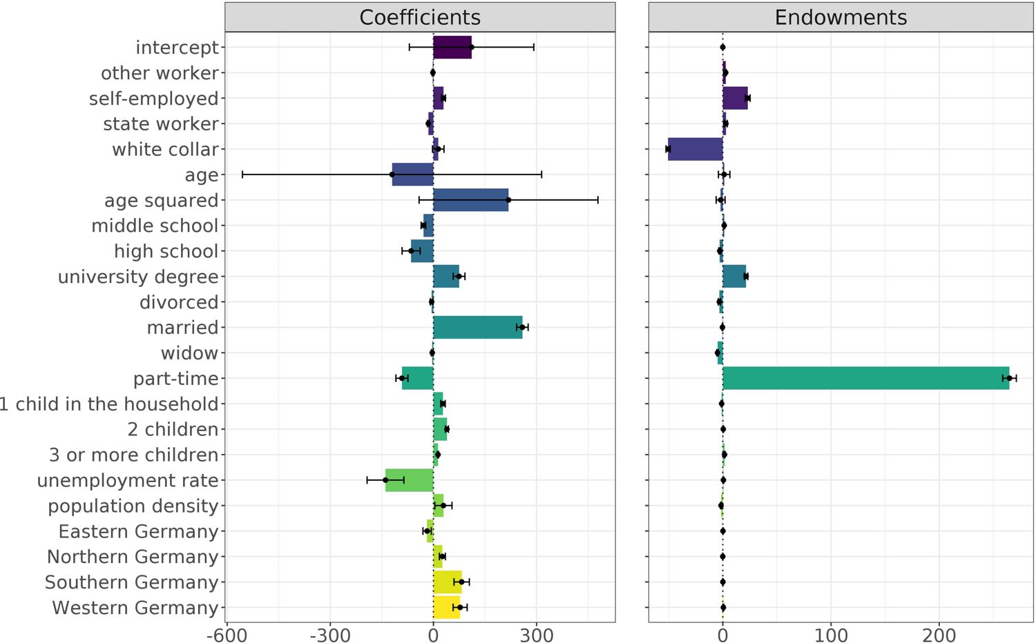
Income gap decomposition by gender15.. Note: The figure shows how far the coefficients (left-hand side) and endowments (right-hand side) widen or narrow the gender income gap. The decomposition results show differences in the magnitude of the coefficients of all independent variables according to gender. While the left-hand side illustrates the effects that narrow the gender income gap, the right-hand side shows the driving forces behind the widening of the gap. The endowments show compo-sitional differences between the sexes. The reducing factors of the income gap are shown on the left-hand side, whereas the drivers of the income gap are illustrated on the right-hand side.For detailed descriptions of the variables and reference categories, see Table A2. Source: own illustration.
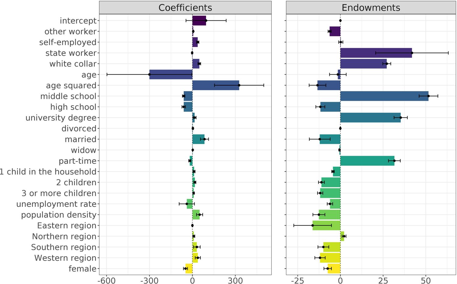
Income gap decomposition by migration status.. Note: The figure shows how far the coefficients (left-hand side) and endowments (right-hand side) widen or narrow the income gap between the migrant and majority population. The decomposition results show differences in the magnitude of the coefficients of all independent variables according to migration. While the left-hand side illustrates the effects that narrow the migrant income gap, the right-hand side shows the driving forces behind the widening of the gap. The endowments show compositional differences between the majority and the migrant population. The reducing factors of the income gap are shown on the left-hand side, whereas the drivers of the migrant income gap are illustrated on the right-hand side. For detailed descriptions of the variables and reference categories, see Table A2. Source: own illustration.

Validation of relative individual income by sex and districts, 2014.. Note: Since the absolute values are on different scales due to the conceptual mismatches and different frames of the underlying datasets, only the comparison of the relative spatial income distributions is meaningful between the three datasets. Darker colors indicate larger individual income medians. Source: own illustration based on Tax Data 2014, INKAR database, and MikroSim.

Working population by region in the base scenario.. Note: The figure shows the simulated working population in millions from 2011 to 2040. The colors indicate regions: East Germany (blue) and West Germany (green). Source: own illustration.

Population by region in the base scenario.. Note: The figure shows the simulated population in millions from 2011 to 2040. The colors indicate regions: East Germany (blue) and West Germany (green). Source: own illustration.

First generation migrants by region in the base scenario.. Note: The figure shows the simulated migrant population in millions from 2011 to 2040. The colors indicate regions: East Germany (blue) and West Germany (green). Source: own illustration.
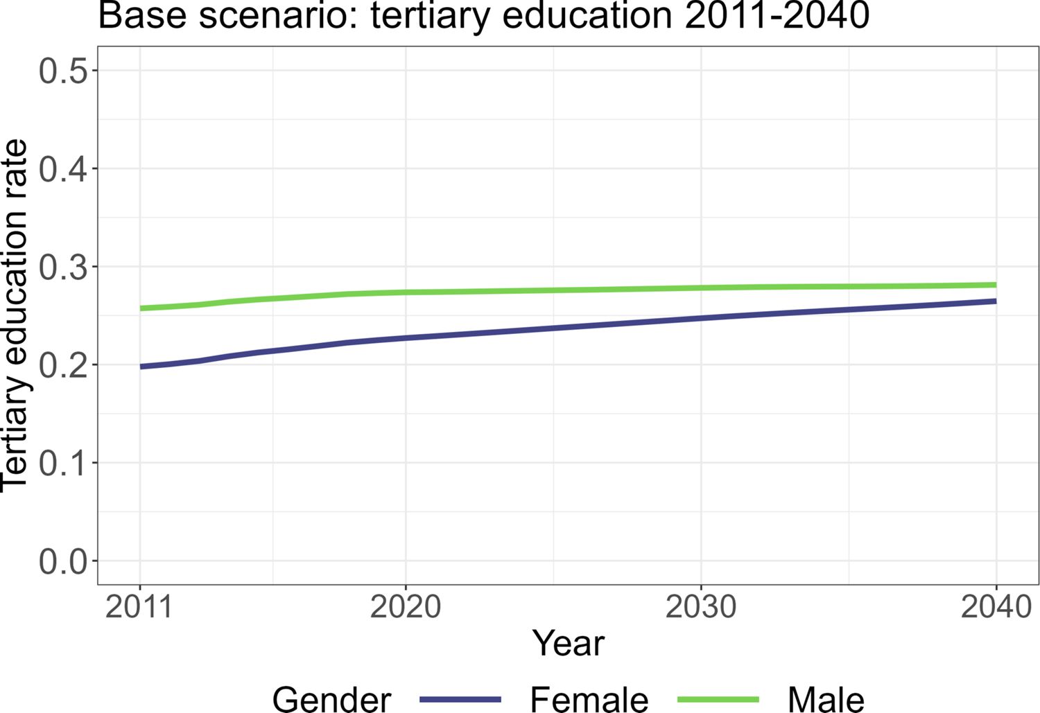
Rate of tertiary education by region in the base scenario.. Note: The figure shows the simulated rate of tertiary education of men (green) and women (blue) in the labor force from 2011 to 2040. Source: own illustration.
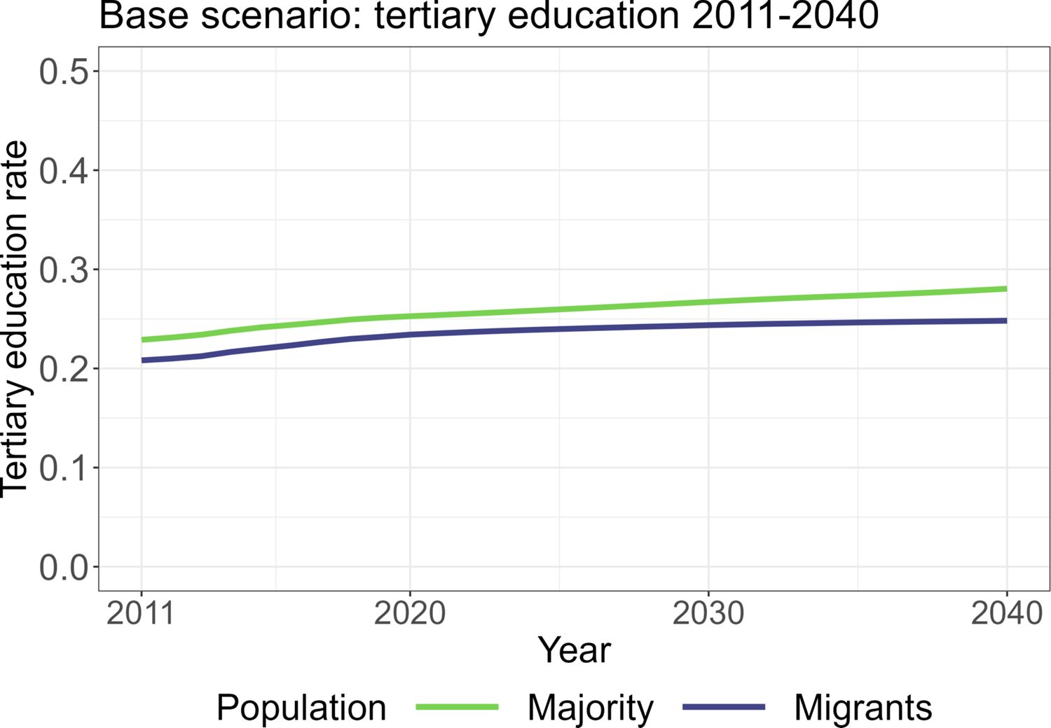
Migrants by region in the base scenario.. Note: The figure shows the simulated rate of tertiary education of the majority population (green) and migrants (blue) in the labor force from 2011 to 2040. Source: own illustration.
Income Estimation in Selected Microsimulation Models*
| Author & Date | Model | Country | Data | Measure | Estimation | Covariates | Alignment | Regional variables |
|---|---|---|---|---|---|---|---|---|
| Andreassen et al. (2020) | MOSART | Norway | Administrative data registers from Norway | Logarithm of labor income | RE models by different cohorts | Age, gender, partnership status, children, (ongoing) education, seniority, pension (type of pension), stable career path, time outside the labor force, year of observation | Demographic modules are aligned to results from Statistics Norway’s official population projections; for years with actual observations aligned to these | No |
| Bonin et al. (2015) | ZEWDMM | Germany | German Socio-Economic Panel (GSOEP) 2009 data of 25 to 29 aged cohort | Logarithm of gross hourly wage | OLS by gender | Education, working experience, firm tenure | No | No |
| Bönke et al. (2020) | Germany | German Socio-Economic Panel (GSOEP) 1964 to 1985 cohorts until age 60 | Lifetime income (logarithm of labor income) | OLS-LDV by gender | Full- and part-time, employment experience, income from last two years, education, marriage, working hours | No | No | |
| Conti et al. (2023) | T-DYMM | Italy | AD-SILC; administrative and longitudinal survey data | Monthly labor income | RE models by occupational group | Differentiated by groups, complete list: gender, born in EU, education, number and ages of children, working experience, working experience†, permanent contract, part-time, employment status of partner | Demographic modules; income aligned to labor productivity growth and consumer price index | No |
| Dekkers et al. (2009) | MIDAS | Belgium, Italy | Belgium: Panel Households (PSBH); Germany: German Socio-Economic Panel (SOEP); Italy: European Community Household Panel (ECHP) | Logarithm of hourly | Belgium: OLS by germany and Italy: RE by gender | Belgium: Age, age†, education; Germany: Potential experience (= age - years in education), potential experience†, education, marital status, firm size, number of children, chronically ill, tenure, public sector; Italy: Potential experience, potential experience†, education, public sector, permanent contract, duration in work | Corrected growth individual hourly wage rates, additional macroeconomic productivity assumptions | No† |
| Emmerson et al. (2004) | Pensim2 | UK | British Household Panel Survey (BHPS) | Earnings | RE models | Work history (including occupation, industry and sector), year of education | No | No |
| Favreault and Smith (2004); Favreault et al. (2015) | DYNASIM III & MINT8 | US | Survey of Income and Program Participation (SIPP), Panel Study of Income Dynamics (PSID), National Longitudinal Survey of Youth (NLSY) | Logarithm of hourly wages for individuals with positive income for the year | RE models by age, gender and race | Marital status, education level, additional age splines, region of residence, disability status, in school, birth cohort, job tenure, education level*age splines, number and ages of children, health status, disability beneficiary status | Wage growth assumptions are used for future periods | Yes |
| Flood (2008) | SESIM III | Sweden | LINDA administrative panel database; SCB income distribution survey and other | Logarithm of full-time earnings | RE models by occupational sector and gender | Working experience, education, marital status, nationality | Only demographics | No |
| Holm et al. (2007) | SVERIGE | Sweden | Base dataset population of Sweden, ASTRID panel database | Relative earnings (lagged monthly earnings divided by the average earnings) | OLS for full- and part-time workers | Age, gender, education, education the year before, regional unemployment rate | Demographic modules are aligned to aggregate indicators from observed data and projections from Statistics Sweden | Yes |
| Income change (yearly change of earnings) | OLS-LDV for six different groups (got unemployed, emigrated, got employed, immigrated, migrated, ordinary group) | Gender, age, education, civil status, former salary, born in Sweden | ||||||
| Schwabish and Topoleski (2013) | CBOLT | US | Data from the Social Security Administration (SSA), Survey of Income and Program Participation (SIPP), Health and Retirement Survey, Current Population Survey (CPS) | Logarithm of annual earnings | RE (Carroll et al., 1992) | Age, gender, lifetime educational attainment, marital status, number of children u. 6, in school, birth cohort, social security benefit status, permanent and transitory shocks | Modules are aligned to demographic and economic projections from Congressional Budget Office (CBO) | NO |
| Zaidi et al. (2009) | SAGE | UK | British Household Panel Survey (BHPS) | Logarithm of monthly earnings | RE models with first-order disturbance terms by gender and qualifications | Recent employment experience, age, age†, education, occupation, industry, partnership status, employment status of partner, restriction of work by health, public or private sector, children living at home, age of youngest child; full- and part-time status | It is possible to add alignment parameters in future versions of the SAGE model. | No |
-
*
This table is not a complete list of all microsimulation models with income modules worldwide, but an attempt to shed light on the "black boxes" of relevant and ongoing microsimulation models. We have only included microsimulation models that can be cited and provide all information for the table shown
-
†
The updated version of MIDAS-BE 2.0 includes regional information on Flanders, the Walloon area and Brussels-Capital region (Dekkers et al., 2023).
Definition of Covariates
| Individual Characteristics | |
|---|---|
| occupational group | blue-collar (reference), other worker, self-employed, |
| state worker, white collar, | |
| age | age in years |
| education | ISCED levels 1 and 2 (middle school), ISCED level 3 (high school), |
| ISCED level 4 (reference), ISCED levels 5 and 6 (= university degree) | |
| family type | divorced, married, widow, single (reference) |
| part time | 1 if individual works part-time, 0 otherwise (full-time) |
| migrant group | born in Germany (reference), late resettlers, |
| Turkey, South-EU, EU before 2004 (without South-EU) | |
| EU after 2004 (including Poland and Croatia), | |
| Former yug. Countries (without Croatia), Africa, | |
| Near and Middle East, South and South-East Asia, | |
| Rest of the world (incl. Russia, America, Rest of Europe) | |
| female | 1 if individual is female, 0 otherwise |
| Household Characteristics | |
| number of kids | 0 (reference), 1, 2, 3 or more |
| Regional Characteristics | |
| share of unemployed | Unemployed persons per 1000 working-age population (Unemployedtime/Employed(15− < 65 years)time * 1000) |
| population density | Inhabitants per squared kilometer inhabitantstime/areatimecontinuous |
| 5 regions of federal states | North, East, South, West, City-States (reference) |
-
Note: *employees are only employees subject to social insurance at the workplace.
Initial income estimation results for men and women
| Dependent variable: | ||
|---|---|---|
| Log Monthly Income | ||
| Male | Female | |
| Intercept | 6.125*** (0.011) | 5.853*** (0.013) |
| Other Worker | 0.397*** (0.003) | 0.276*** (0.004) |
| Self Employed | 0.094*** (0.002) | 0.096*** (0.004) |
| State-Worker | 0.280*** (0.003) | 0.554*** (0.005) |
| White Collar | 0.098*** (0.001) | 0.185*** (0.002) |
| Age | 0.058*** (0.0005) | 0.065*** (0.001) |
| Age Squared | 0.001*** (0.00001) | 0.001*** (0.00001) |
| ISCED Levels 1 and 2 | 0.326*** (0.003) | 0.331*** (0.003) |
| ISCED Level 3 | 0.116*** (0.002) | 0.154*** (0.002) |
| ISCED Level 5 | 0.142*** (0.003) | 0.088*** (0.003) |
| Late resettlers | 0.095*** (0.004) | 0.073*** (0.004) |
| Turkey | 0.069*** (0.005) | 0.101*** (0.008) |
| South-EU | 0.094*** (0.007) | 0.084*** (0.010) |
| EU before 2004 | 0.054*** (0.009) | 0.028** (0.011) |
| EU after 2004 | 0.147*** (0.005) | 0.112*** (0.006) |
| Former Yugoslavia | 0.113*** (0.008) | 0.081*** (0.010) |
| Africa | 0.220*** (0.012) | 0.105***(0.020) |
| Middle East | 0.123*** (0.008) | 0.089***(0.010) |
| South-East-Asia | 0.169*** (0.010) | 0.157*** (0.011) |
| Rest of the World | 0.127*** (0.007) | 0.126*** (0.007) |
| Married | 0.157*** (0.002) | 0.160*** (0.003) |
| Divorced | 0.013*** (0.003) | 0.055*** (0.003) |
| Widow | 0.119*** (0.009) | 0.223*** (0.003) |
| Part-time | 0.542*** (0.002) | 0.457*** (0.002) |
| 1 Child in Household | 0.036*** (0.002) | 0.037*** (0.002) |
| 2 Children in Household | 0.104*** (0.002) | 0.037*** (0.003) |
| 3 or more Children | 0.159*** (0.004) | 0.032*** (0.005) |
| Unemployment Rate | 0.002*** (0.0001) | 0.002*** (0.0001) |
| Population Density | 0.00003*** (0.00000) | 0.0001*** (0.00000) |
| East | 0.120*** (0.004) | 0.008(0.005) |
| North | 0.066*** (0.004) | 0.019*** (0.005) |
| South | 0.088*** (0.004) | 0.006 (0.005) |
| West | 0.089*** (0.004) | 0.011** (0.004) |
| Number of Individuals | 344,463 | 318,102 |
| var(Ind) | 0.157 | 0.193 |
| var(Residuals) | 0.076 | 0.105 |
| Observations | 635,492 | 573,659 |
| Log Likelihood | 340,397.200 | 389,648.800 |
| Akaike Inf. Crit. | 680,864.300 | 779,367.700 |
| Bayesian Inf. Crit. | 681,262.000 | 779,761.800 |
-
Notes: Standard errors given in parenthesis. ∗p<0.05; ∗∗p<0.01; ∗∗∗p<0.001.
Forecast income estimation results for men and women
| Dependent variable: | ||
|---|---|---|
| Log Monthly Income | ||
| Male | Female | |
| Intercept | 3.134*** (0.013) | 2.929***(0.015) |
| Previous Log Income | 0.571*** (0.001) | 0.570***(0.001) |
| Other Worker | 0.271*** (0.004) | 0.198***(0.004) |
| Self Employed | 0.054*** (0.002) | 0.046***(0.004) |
| State-Worker | 0.121*** (0.003) | 0.256***(0.004) |
| White Collar | 0.055*** (0.002) | 0.109***(0.003) |
| Age | 0.004*** (0.0004) | 0.010***(0.001) |
| Age Squared | 0.00003*** (0.00001) | 0.0001***(0.00001) |
| ISCED Levels 1 and 2 | 0.147*** (0.003) | 0.130***(0.003) |
| ISCED Level 3 | 0.048*** (0.003) | 0.063***(0.003) |
| ISCED Level 5 | 0.097*** (0.003) | 0.074***(0.003) |
| University Graduation | 0.014*** (0.003) | 0.029***(0.004) |
| Late resettlers | 0.039*** (0.003) | 0.031***(0.004) |
| Turkey | 0.005 (0.005) | 0.032***(0.007) |
| South-EU | 0.015** (0.006) | 0.024***(0.009) |
| EU before 2004 | 0.023*** (0.008) | 0.006 (0.010) |
| EU after 2004 | 0.062*** (0.005) | 0.035***(0.005) |
| Former Yugoslavia | 0.045*** (0.007) | 0.032***(0.009) |
| Africa | 0.065*** (0.011) | 0.008 (0.020) |
| Middle East | 0.032*** (0.008) | 0.064***(0.011) |
| South-East-Asia | 0.070*** (0.010) | 0.069***(0.010) |
| Rest of the World | 0.062*** (0.007) | 0.050***(0.007) |
| Married | 0.060*** (0.002) | 0.058***(0.002) |
| Divorced | 0.010*** (0.003) | 0.032***(0.003) |
| Widow | 0.048*** (0.008) | 0.128***(0.005) |
| Part-time | 0.286*** (0.002) | 0.265***(0.002) |
| 1 Child in Household | 0.031*** (0.002) | 0.028***(0.002) |
| 2 Children in Household | 0.062*** (0.002) | 0.054***(0.003) |
| 3 or more Children | 0.097*** (0.004) | 0.068***(0.005) |
| Unemployment Rate | 0.001*** (0.00005) | 0.0005***(0.0001) |
| Population Density | 0.00001*** (0.00000) | 0.00002***(0.00000) |
| East | 0.060*** (0.004) | 0.006 (0.004) |
| North | 0.031*** (0.004) | 0.015***(0.004) |
| South | 0.042*** (0.004) | 0.018***(0.004) |
| West | 0.042*** (0.003) | 0.017***(0.004) |
| Number of Individuals | 194,132 | 174,839 |
| var(Ind) | 0.003 | 0.003 |
| var(Residuals) | 0.119 | 0.154 |
| Observations | 307,605 | 272,851 |
| Log Likelihood | 113,292.900 | 134,186.900 |
| Akaike Inf. Crit. | 226,659.800 | 268,447.800 |
| Bayesian Inf. Crit. | 227,053.400 | 268,836.900 |
-
Note: Standard errors given in parenthesis. ∗p<0.05; ∗∗p<0.01; ∗∗∗p<0.001.
Descriptive Statistics of Individual Net Income
| 20%-Q | 40%-Q | 60%-Q | 80%-Q | Mean | SD | |
|---|---|---|---|---|---|---|
| Female | 700 | 1,000 | 1,400 | 1,900 | 1,400 | 1,400 |
| Male | 1,200 | 1,700 | 2,100 | 3,000 | 2,300 | 2,600 |
| Migrants | 800 | 1,200 | 1,600 | 2,200 | 1,600 | 1,300 |
| Majority population | 900 | 1,400 | 1,800 | 2,500 | 1,900 | 2,200 |
-
Note: Q means quantile. SD means standard deviation. Values are provided in Euro and refer to monthly net income (rounded to hundreds) based on generalized Pareto interpolation.
-
Source: Microcensus 2014.
Descriptive Statistics of the Covariates
| Covariates | 2011 | 2040 |
|---|---|---|
| Blue Collar | 7,268,341 | 9,035,568 |
| Other Worker | 6,851,373 | 2,329,589 |
| Self Employed | 3,491,204 | 3,513,550 |
| State-Worker | 1,795,529 | 2,039,539 |
| White Collar | 20,442,203 | 26,469,607 |
| ISCED Levels 1 and 2 | 32,941,690 | 29,983,438 |
| ISCED Level 3 | 16,727,562 | 18,786,855 |
| ISCED Level 4 (post-secondary) | 14,408,798 | 16,856,388 |
| ISCED Level 5 | 4,723,944 | 5,343,423 |
| Single | 32,186,460 | 35,449,969 |
| Divorced | 5,099,718 | 5,954,598 |
| Married | 30,730,796 | 27,663,157 |
| Widow | 1,949,041 | 2,352,947 |
| Part-time | 9,047,698 | 11,373,085 |
| 1 Child in Household | 5,452,759 | 5,461,470 |
| 2 Children in Household | 3,649,681 | 3,598,167 |
| 3 or more Children | 1,770,310 | 2,780,059 |
| City | 5,703,399 | 6,207,812 |
| East | 13,082,995 | 13,012,529 |
| North | 10,290,519 | 10,628,254 |
| South | 22,997,750 | 24,295,421 |
| West | 28,781,700 | 29,496,169 |
| Germans (working age) | 46,644,839 | 45,461,984 |
| Late resettlers | 2,492,969 | 2,195,640 |
| Turkey | 897,308 | 1,444,008 |
| South-EU | 695,417 | 1,175,148 |
| EU before 2004 | 407,257 | 623,370 |
| EU after 2004 | 650,194 | 1,273,984 |
| Former Yugoslavia | 295,555 | 502,382 |
| Africa | 127,658 | 244,669 |
| Middle East | 173,182 | 331,790 |
| South-East-Asia | 180,834 | 365,227 |
| Rest of the World | 535,904 | 917,020 |
-
Note: The table includes only first-generation working-age migrants.
References
-
1
The immigrant-native wage gap in GermanyJahrbücher Für Nationalökonomie Und Statistik 232:490–517.https://doi.org/10.1515/jbnst-2012-0502
-
2
Mikrosim codebase, version 2.1.4Gitlab.
-
3
The Migrant Pay Gap: Understanding Wage Differences Be-Tween Migrants and NationalsGeneva: International Labour Organization.
-
4
The dynamic cross-sectional microsimulation model MOSARTInternational Journal of Microsimulation 13:92–113.https://doi.org/10.34196/ijm.00214
-
5
Parenthood and the gender gap in payJournal of Labor Economics 34:545–579.https://doi.org/10.1086/684851
-
6
Wage performance of immigrants in GermanyGerman Economic Review 20:e141–e169.https://doi.org/10.1111/geer.12159
-
7
Wage discrimination: reduced form and structural estimatesThe Journal of Human Resources 8:436.https://doi.org/10.2307/144855
-
8
Wie Groß Ist Der Gender Gap? Anspruch Und Wirklichkeit Der Gleichstel-Lungspolitik28–33, Zementiertes Rollenverhalten in Der Fürsorge Für Kinder, Trotz Pandemie–Eine Herausforderung Für Die Familien-Und Gleichstellungspolitik, Wie Groß Ist Der Gender Gap? Anspruch Und Wirklichkeit Der Gleichstel-Lungspolitik, p.
-
9
Life-Cycle Incidence of Family Policy Measures in Germany: Evidence from a Dynamic Microsimulation ModelSOEPpapers 770, Berlin: DIW Berlin.
-
10
Wer Gewinnt? Wer Verliert? Die En-Twicklung Und Prognose von Lebenserwerbseinkommen in DeutschlandGütersloh: Bertelsmann Stiftung.
- 11
-
12
Der einfluss der beruflichen geschlechtersegregation auf den “gender pay gap”: zur bedeutung geschlechtlich konnotierter arbeitsinhalteKZfSS Kölner Zeitschrift Für Soziologie Und Sozialpsychologie 65:301–338.https://doi.org/10.1007/s11577-013-0201-1
-
13
The buffer-stock theory of saving: some Macroeconomic evidenceBrookings Papers on Economic Activity 1992:61–156.https://doi.org/10.2307/2534582
-
14
Returns-to-education gaps between native and migrant workers: the infl uence of economic integration on their drivers. are active labour market policies (ALMPs) an eff ective remediation tool? A case comparison: Italy, Germany, Denmark and cyprusBulletin of Geography. Socio-Economic Series 56:63–81.https://doi.org/10.12775/bgss-2022-0013
-
15
Social theory, social research, and a theory of actionAmerican Journal of Sociology 91:1309–1335.https://doi.org/10.1086/228423
-
16
Linking CGE and microsimulation models: a comparison different approachesInternational Journal of Microsimulation 3:72–91.https://doi.org/10.34196/ijm.00026
-
17
Working Papers 1, Rome: Ministry of Economy and Finance, Department of the TreasuryWorking Papers 1, Rome: Ministry of Economy and Finance, Department of the Treasury.
-
18
ENEPRI research report 65, Brussels: European Network of Economic PolicyENEPRI research report 65, Brussels: European Network of Economic Policy.
-
19
New Pathways in Microsimulation287–304, What are the driving forces behind trends in inequality among pensioners? Validating MIDAS Belgium using a stylized model, New Pathways in Microsimulation, London, Routledge, p.
-
20
Projections of the Gender Pen-Sion Gap in Belgium Using MIDAS (Project MIGAPE, Work Package 3)MI-GAPE research project, Brussel: Federaal Planbureau, Economische analyses en vooruitzichten.
-
21
Impact on pension outcomes of life events: standard sim-ulations from five European countriesMIGAPE research project, Brussels: Center for European Policy Studies (CEPS).
-
22
MIDAS 2.0: Revisie van Een Dynamisch MicrosimulatiemodelWorking Paper 2-23, Brussel: Federaal Planbureau, Economische analyses en vooruitzichten.
-
23
Tax-Benefit Systems and the Gender Gap in IncomeIZA Discussion Paper Series 13786, Bonn: IZA Institute of LaborEconomics.
-
24
An Assessment of Pensim2IFS Working Paper Series 04/21, London: Institute for Fiscal Studies.
-
25
The influence of migration patterns on regional demographic development in GermanySocial Sciences 12:255.https://doi.org/10.3390/socsci12050255
-
26
A Primer on the Dynamic Simulation of Income Model (DYNASIM3): The Retirement Project. An Urban Institute Issue FocusDiscussion Papers, Washington, DC: The Urban Institute.
-
27
The Dynamic Simulation of Income Model DYNASIM: An OverviewResearch Report, Washington, DC: The Urban Institute.
-
28
Simulating an ageing population: A microsimulation approach applied to sweden, contributions to economic analysis55–83, Chapter 3 SESIM: A Swedish micro-simulation model, Simulating an ageing population: A microsimulation approach applied to sweden, contributions to economic analysis, Bingley, Emerald, p.
-
29
Where do women earn more than men? Explaining regional differences in the gender pay gapJournal of Regional Science 61:1065–1086.https://doi.org/10.1111/jors.12532
-
30
Wie Groß Ist Der Gender Gap? Anspruch Und Wirklichkeit Der Gleichstellungspolitik8–13, Who cares? Arbeitsteilung in familien als letzte hürde auf dem weg zur gleichberechtigung, Wie Groß Ist Der Gender Gap? Anspruch Und Wirklichkeit Der Gleichstellungspolitik, p.
-
31
Effekte der gruppengröße auf die arbeitsmarktintegration von migrantenKZfSS Kölner Zeitschrift Für Soziologie Und Sozialpsychologie 61:387–409.https://doi.org/10.1007/s11577-009-0073-6
-
32
A work in progress: p rospects for upward mobility among new immigrants in GermanyWashington, DC: Migration Policy Institute.
-
33
Wie Groß Ist Der Gender Gap? Anspruch Und Wirklichkeit Der Gleichstellungspolitik13–17, Gender pay gap: ursachen und maßnahmen, Wie Groß Ist Der Gender Gap? Anspruch Und Wirklichkeit Der Gleichstellungspolitik, p.
-
34
Can regional gender ideologies account for variation of gender pay gaps? The case of GermanySocial Sciences 10:347.https://doi.org/10.3390/socsci10090347
-
35
Long-term trends in the gender income gap within couples: West Germany, 1978–2011Social Politics 29:980–1008.https://doi.org/10.1093/sp/jxac019
-
36
Wie Groß Ist Der Gender Gap? Anspruch Und Wirklichkeit Der Gleichstellungspolitik36–40, Frauen als Gründerinnen: Die Covid-Pandemie vergrößert den bestehenden Gender Gap, Wie Groß Ist Der Gender Gap? Anspruch Und Wirklichkeit Der Gleichstellungspolitik, p.
-
37
Dealing with space and place in standard survey dataSurvey Research Methods 11:267–287.
-
38
Is There a Gap in the Gap? Regional Differences in the Gender Pay GapScottish Journal of Political Economy 60:412–439.https://doi.org/10.1111/sjpe.12017
-
39
Oaxaca: Blinder-Oaxaca Decomposition in RBratislava, Slovakia: Social Policy Institute.
-
40
Economic-demographic effects of immigration: results from a dynamic spatial microsimulation modelInternational Regional Science Review 27:379–410.https://doi.org/10.1177/0160017604267628
-
41
Model 19 SVERIGE543–549, Modelling Our Future: Population Ageing Health, and Aged Care International symposia in economic theory and econometrics, Model 19 SVERIGE, Boston, Mass: Elsevier B.V, p.
-
42
Regionale Ungleichheit in Deutschland: Wo leben die Reichen und wo die Armen?Ifo Schnelldienst 73:43–47.
-
43
The Immigrant-Native Wage Gap in Germany RevisitedSSRN Electronic Journal, Bonn, IZA Institute of Labor Economics, 10.2139/ssrn.3401126.
-
44
Between Mechanism Talk And Mechanism Cult: New Emphases in Explanatory Sociology And Empirical ResearchKZfSS Kölner Zeitschrift Für Soziologie Und Sozialpsychologie 66:91–115.https://doi.org/10.1007/s11577-014-0272-7
-
45
MIGAPE research project Liechtenstein: University of LiechtensteinMIGAPE research project Liechtenstein: University of Liechtenstein.
-
46
Child Penalties across Countries: Evidence and ExplanationsNBER Working Paper Series 25524, Cambridge, Massachusetts: National Bureau of Eco-nomic Research.
-
47
Projections of the Gender Pension Gap in Slovenia Using DYPENSI (Project MIGAPE, Work Package 3)MIGAPE research project, Ljubljana: Institute for Economic Research.
-
48
Lohnungleichheiten zwischen Akademikerinnen und Akademikern: Der Einfluss von fachlicher Spezialisierung, frauendominierten Fächern und beruflicher Segregation / Wage Inequality between Male and Female University Graduates: The Influence of Occupational Specialization, Female-Dominated Subjects and Occupational SegregationZeitschrift Für Soziologie 38:262–281.https://doi.org/10.1515/zfsoz-2009-0401
-
49
Gender Pay Gaps in the European Union: A Statistical Analysis. Statistical Working PapersLuxembourg: European Union, Eurostat.
-
50
Projections of the Gender Pension Gap in Luxembourg Using MIDAS_LU 2020Luxembourg: Luxembourg Institute of Socio-Economic Research.
-
51
Regression-Style Models for Parameter Estimation in Dynamic Microsimulation: An Empirical Performance AssessmentInternational Journal of Microsimulation 8:83–127.https://doi.org/10.34196/ijm.00117
-
52
Investment in human capital and personal income distributionJournal of Political Economy 66:281–302.https://doi.org/10.1086/258055
-
53
Schooling, Experience, and Earnings: Human Behavior & Social Institutions No.2Cambridge, Massachusetts National Bureau of Economic Research.
-
54
Financial and Social Sustainability of the Portuguese Pension SystemEstudos da fundação, Lisboa: Francisco Manuel dos Santos Foundation.
-
55
A Population Based Regional Dynamic Microsimulation of Germany: The MikroSim ModelMethods, Data, Analyses 15:241–264.
-
56
Smaller differences in bigger cities? Assessing the regional dimension of the gender wage gapEuropean Sociological Review 33:292–3044.https://doi.org/10.1093/esr/jcx037
-
57
Male-female wage differentials in urban labor marketsInternational Economic Review 14:693.https://doi.org/10.2307/2525981
- 58
-
59
Practical Microsimulation ModellingOxford: Oxford University Press.https://doi.org/10.1093/oso/9780198852872.001.0001
- 60
- 61
-
62
A New Type of Socio-Economic SystemThe Review of Economics and Statistics 39:116–123.https://doi.org/10.2307/1928528
- 63
-
64
Wie Groß Ist Der Gender Gap? Anspruch Und Wirklichkeit Der Gleichstellungspolitik3–5, Das geschlechtsspezifische einkommensgefälle entlang der einkommensverteilung in Deutschland, Wie Groß Ist Der Gender Gap? Anspruch Und Wirklichkeit Der Gleichstellungspolitik, p.
-
65
Urban effects on participation and wages: are there gender differences?Journal of Urban Economics 58:513–536.https://doi.org/10.1016/j.jue.2005.08.006
-
66
Microsimulation methods for population projectionPopulation Vol. 53:97–136.https://doi.org/10.3917/popu.p1998.10n1.0136
- 67
-
68
Migration and Wage Inequality: A Detailed Analysis for German Regions over Time. Hohenheim Discussion Papers in Business, Economics and Social Sciences 04-2022Stuttgart: Faculty of Business, Economics and Social Sciences, University of Hohenheim.
-
69
Mikrosimulationen: methodische grundlagen und ausgewählte anwendungsfelder35–56, Neuere bevölkerungsbezogene mikrosimulationen in großbritannien und Deutschland, Mikrosimulationen: methodische grundlagen und ausgewählte anwendungsfelder, Wiesbaden, Springer, p, 10.1007/978-3-658-23702-8.
-
70
Working Paper Series 2013-04, Washington, D.C.: Congressional Budget officeWorking Paper Series 2013-04, Washington, D.C.: Congressional Budget office.
-
71
What is social science microsimulation?Social Science Computer Review 29:9–20.https://doi.org/10.1177/0894439310370085
- 72
-
73
Gender Pay Gap 2021: Germany remainsamong EU states with highest disparityhttps://www.destatis.de/Europa/EN/Topic/Population-Labour-Social-Issues/Labour-market/gender_pay_gap.html, Accessed, 15 March 2023.
-
74
Unbereinigter Gender Pay Gap (GPG) nach Gebietsstand ab 1995https://www.destatis.de/DE/Themen/Arbeit/Verdienste/Verdienste-GenderPayGap/Tabellen/ugpg-01-gebietsstand.html, Accessed, 6 March 2023.
-
75
Bonn: Bundeszentrale für politische BildungBonn: Bundeszentrale für politische Bildung.
-
76
New Frontiers in Microsimulation Modelling351–379, Employment transitions and earnings dynamics in the SAGE model, New Frontiers in Microsimulation Modelling, London: Routledge, p.
- 77
Article and author information
Author details
Monika Obersneider

Funding
The research is funded by the German Research Foundation as part of the research unit FOR 2559 MikroSim.
Acknowledgements
We would like to thank Petra Stein and Ralf Münnich for their valuable advice, as well as the participants of the European Meeting of the International Microsimulation Association 2022 and the Joint Statistical Meetings 2022. We appreciate the careful proofreading by Anthony Daykin and Leonie Schröder and are very grateful to the two anonymous reviewers for their detailed and constructive comments on the original submission to the International Journal of Microsimulation. The research was carried out as part of the research unit FOR 2559 MikroSim. We thank the German Research Foundation for funding.
Publication history
- Version of Record published: April 30, 2024 (version 1)
Copyright
© 2024, Emmenegger and Obersneider
This article is distributed under the terms of the Creative Commons Attribution License, which permits unrestricted use and redistribution provided that the original author and source are credited.