
Equivalent Static Wind Load for Structures with Inerter-Based Vibration Absorbers

1
Tianjin Research Institute for Water Transport Engineering, Ministry of Transport of People’s Republic of China, Tianjin 300456, China
2
School of Civil Engineering and Architecture, Northeast Electric Power University, Jilin 132012, China
3
National Institute of Technology (KOSEN), Akita College, Akita 011-8511, Japan
*
Author to whom correspondence should be addressed.
Wind 2022, 2(4), 766-783; https://doi.org/10.3390/wind2040040
Submission received: 10 November 2022
/
Revised: 2 December 2022
/
Accepted: 9 December 2022
/
Published: 12 December 2022
Abstract
:Equivalent Static Wind Loads (ESWL) are desired in structural design to consider peak dynamic wind effects. Conventional ESWLs are for structures without control. For flexible structures with vibration control devices, the investigation of ESWL is required. Inerter-based Vibration Absorbers (IVAs), due to the light weight and high performance, gained much research attention recently. This paper established a generic analytical framework of ESWL for structures with IVAs. The analytical optimal design formulas for IVAs with different configurations and installation locations are provided. Subsequently, the solutions to uncontrolled and controlled wind-induced responses are derived based on the filter approach. Finally, the ESWL for controlled structures are presented with a gust response factor approach. The ESWL estimation for a tall chimney controlled by IVAs is illustrated, and the results revealed a significant ESWL reduction effect of the IVAs, particularly for the cross-wind vortex resonance. In the presented framework, the conventional uncontrolled ESWL can be converted to the controlled one with a control ratio. The closed form solution of the control ratio is provided, which enables a quick estimation of ESWL for controlled structures particularly in the preliminary design stage. The presented approach has the potential to be extended to more complex structures and vibration control devices.
1. Introduction
The Equivalent Static Wind Load (ESWL) is an important concept in structural wind resistance designs. It provides a simplified procedure to estimate the peak dynamic wind effect on structures, which can be combined with other load effects in structural design. The basic framework of ESWL was proposed as gust loading factors by Davenport [1]. The ESWL concept and method have been extensively developed and extended considering more complex situations [2,3,4,5,6,7,8,9,10,11,12,13,14,15]. These studies provide a basis for international codes for wind loading [16,17]. However, these ESWL approaches are for structures without vibration control.
The development on material and construction technologies enables structures to become more flexible. Vibration control devices are commonly applied to modern structures. Tuned Mass Damper (TMD) is one of the most classical Dynamic Vibration Absorbers (DVAs) for reducing the vibration responses of flexible structures. The vibration control performances are strongly dependent on the tuning parameters. Den Hartog [18] proposed a theoretic framework to obtain the optimal parameters analytically, which aims at minimizing the norms of the dynamic amplification functions. Based on the theory, the analytical optimal parameters of TMD for harmonic and white-noised excitations are derived [19]. According to this criterion, the control performance of the TMD is highly dependent on the tuning mass ratio. Achieving a lightweight design of the DVA is a challenging task.
In order to further enhance the vibration control performance, many investigations were performed. The inerter device was invented for both mechanical and civil engineering fields [20,21]. It can produce a control force in proportion to the relative acceleration at its two ends implemented by proper mechanical configurations, such as a rack-pinon-flywheel, screw-ball systems, etc. [22]. Thus, an inertial effect of thousands of times its physical mass can be provided by an inerter. The Inerter-based Vibration Absorbers (IVAs) have the potential to achieve lightweight and high performance vibration control, which has recently attracted much attention in research.
The first IVA realized in practical civil engineering structures is the Tuned Mass Viscous Damper (TVMD) [21], which is installed on a tall building located in Sendai, Japan. Replacing the dashpot of the TMD with TVMD, a Rotational inertia double-tuned mass damper (RIDTMD) [23] was proposed, which significantly reduces the mass of the DVA [24]. Other than TVMD, many other IVA configurations are proposed and investigated. The Tuned Mass Damper Inerter (TMDI) was proposed by adding an inerter between the mass block of the TMD and the ground [25], which is beneficial in base-isolation system [26,27]. Considering the practical installation, the connection of the inerter of TMDI was moved from the ground to the structure body [28,29] to form an inter-layer device, or adjacent buildings, forming a damped link [30,31]. Replacing the mass of the TMD with an inerter, Tuned Inerter Dampers (TIDs) were implemented and investigated [32,33]. A variant design of the above mentioned DVA was achieved to enhance the control performance by connecting the dashpot to the other side. Such as a variant design of TMD (VTMD, [34,35]), a variant design of TMDI (VTMDI, [28,36]) is similar. It is interesting to find that the TVMD and TID forms a variant design pair, and they are extensively compared with each other in the literature [37,38,39]. More recently, the above DVAs are investigated considering nonlinearity effects, such as [40,41].
Although both the IVAs and ESWLs are extensively addressed, they are investigated separately. Because the practical application of IVAs becomes common, it is hoped to develop the corresponding ESWLs for controlled structures. In order to address this gap, the present paper aims at establishing a generic analytical framework of ESWL for structures with IVAs. The analytical optimal design formulas for IVAs with different configurations and installation locations are provided. Subsequently, the solutions to uncontrolled and controlled wind-induced responses are derived based on the filter approach [42]. Finally, the ESWLs for controlled structures are presented with a gust response factor approach. As an example of the application, the ESWL estimation for a tall chimney controlled by IVAs is performed at the end of the paper.
2. Inerter-Based Vibration Absorbers
The equivalent static wind load (ESWL) is based on the wind-induced peak response. For the structures coupling with inerter-based vibration absorbers (IVAs), the wind-induced responses are controlled. Moreover, the control performance of the IVA is highly dependent on the tuning parameters. Therefore, it is the basic task to establish the equations of motion, and determine the optimal parameters and performances of IVA. In this section, a variety of IVAs are formulated generically. The optimal parameters are analytically obtained with the Fixed-point approach.
2.1. Generic Equations of Motion
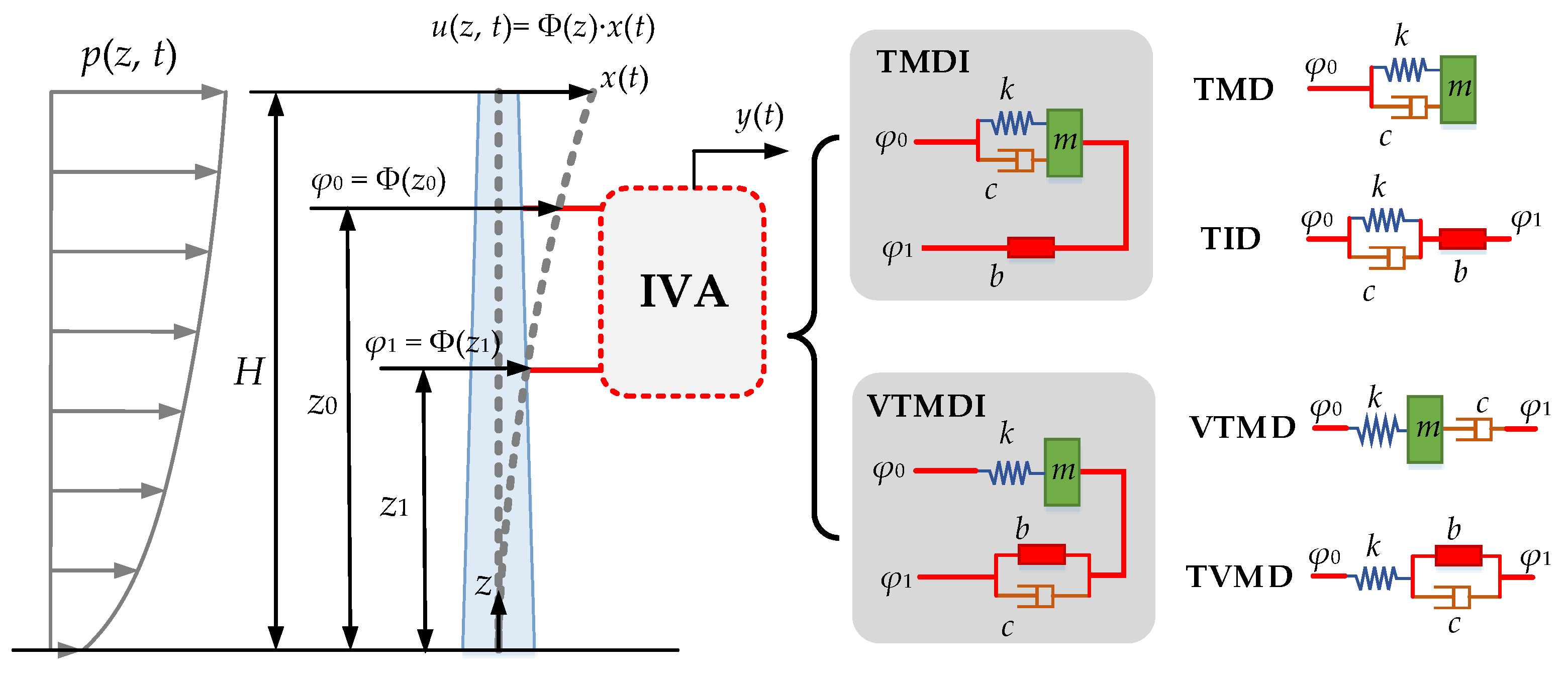
In order to simplify the derivation, the primary structure is assumed to be a generalized single-degree-of-freedom (SDOF) structure. Assuming that the fundamental mode dominates a slender structure as an example, the equation of motion is described with the generalized mass, stiffness, and damping, denoted as M, K, and C, respectively. It is dynamically characterized by the natural circular frequency , and damping ratio . As shown in Figure 1, the displacement response time–history u(z, t) can be decoupled as a spatial variant normalized modal function Φ(z), with respect to the generalized coordinate (height) z (0 ≤ z ≤ H, Φ(H) = 1), and a time dependent generalized displacement response x(t), i.e., u(z, t) = Φ(z)·x(t). Note that x(t) is exactly equalled to the top displacement, x(t) = u(H, t).
For an uncontrolled primary structure subjected to wind load p(z,t), the vibration is governed by Equation (1). In the equation, is the generalized wind load. The wind load is composed of static and dynamic components, statistically denoted by the mean value and standard deviation value . The normalized transfer function H(s) based on the Laplace transform of Equation (1) is written as Equation (2), with s being the complex frequency, and X(s) and F(s) being the Laplace transform of the output response x(t) and the input excitation F(t), respectively. When s takes the pure imaginary frequency iω, H(iω) is the normalized frequency response function. V(s) = is the inverse of H(s). Here, is an imaginary unit. Consequently, the static and dynamic wind-induced responses, denoted by the mean and standard deviation values, and , are shown in Equation (3). The peak response is obtained from the peak factor approach, as shown in Equation (3). According to Davenport’s statistical approach [1], the peak factor g is approximated with , where T is the time duration, n0 is the mean up-crossing rate that can be approximated by , and γ is the Euler constant taken as 0.5772.
In this paper, two major configurations of IVAs, TMDI, and VTMDI are considered, as shown in Figure 1. It is also noted that TMD and TID can be expressed as TMDI with an absent of mass. Likewise, VTMD and TVMD can be VTMDI with an absent of mass. Therefore, these configurations are the major IVAs with similar components and different configurations. They can be formulated and modeled generically. Although the IVAs are discussed in several papers [37,38,39], the ESWL of structures with these IVAs is not fully addressed.
For a primary structure controlled by an IVA installed between coordinates z0 and z1, as shown in Figure 1, the Ritz-Galerkin method is adopted, as referred to [29,39,43,44], assuming that u(z, t) = Φ(z)·x(t). According to the principle of visual work, the equations of motion are rewritten as Equation (4). In the equation, and are the location parameters of the IVA. f0 and f1 are the control force generated by the IVA at installation locations z0 and z1, respectively. y represents the absolute displacement of the IVA.
Considering a Tuned Mass Damper Inerter (TMDI) with mass m, stiffness k, damping c, and inertance coefficients b as an example, f0 and f1 are written in Equation (5). Note that when b = 0, it become a Tuned Mass Damper (TMD). Whereas, when the mass can be ignored (m = 0), it has a similar configuration with a Tuned Inerter Damper (TID). Thus, Equation (5) is applicable for all of the above-mentioned situations. If the dashpot of the TMDI is connected to the inerter side, a variant design of TMDI is formed, namely VTMDI. In this case, f0 and f1 are expressed as Equation (6). When the inerter is absent, it forms a variant design of TMD (VTMD). When the mass becomes absent, it has a similar configuration with the Tuned Viscous Mass Damper (TVMD [21]), which is also denoted as TID2 in [37]. Equation (6) is applicable for these variants. Also note that, when φ1 = 0, the IVAs are connected to the ground, known as grounded IVAs. Conventional IVAs usually takes φ0 = 1 and φ1 = 0 regardless of the installation locations. They are assumed to be connected between the tip of the building and the ground.
Substituting Equation (5) or Equation (6) into Equation (4), we can obtain the normalized transfer function H(s). H(s) can be formatted as a rational expression, as Equation (7). The denominator polynomial is quartic, with dimensionless coefficients γj (j = 0, 1, 2, 3, 4). The numerator polynomial is quadratic, with dimensionless coefficients θj (j = 0, 1, 2).
In order to express the equations in a dimensionless form, the tuning parameters of the IVA are defined, as shown in Table 1.
For TMDI and VTMDI, the coefficients are expressed, as shown in Table 2. Consequently, the controlled wind-induced responses can be calculated by Equation (3), merely adopting the normalized transfer function H(s) as Equation (7).
2.2. Analytical Optimal Design Based on Fixed-Point Approach
The next step is to determine the appropriate parameters of the IVA. Basically, the optimal design is to determine the optimal tuning parameters {νopt, ζdopt} with respect to the input parameters {μ, β, φ0, φ1}. The optimization can be performed based on different performance targets, e.g., the maximum (infinity norm) or 2nd norm of the dynamic amplification function (H∞, H2 optimization). Among them, the most basic optimal design method is the Fixed-point approach (FPA), which can lead to analytical results.
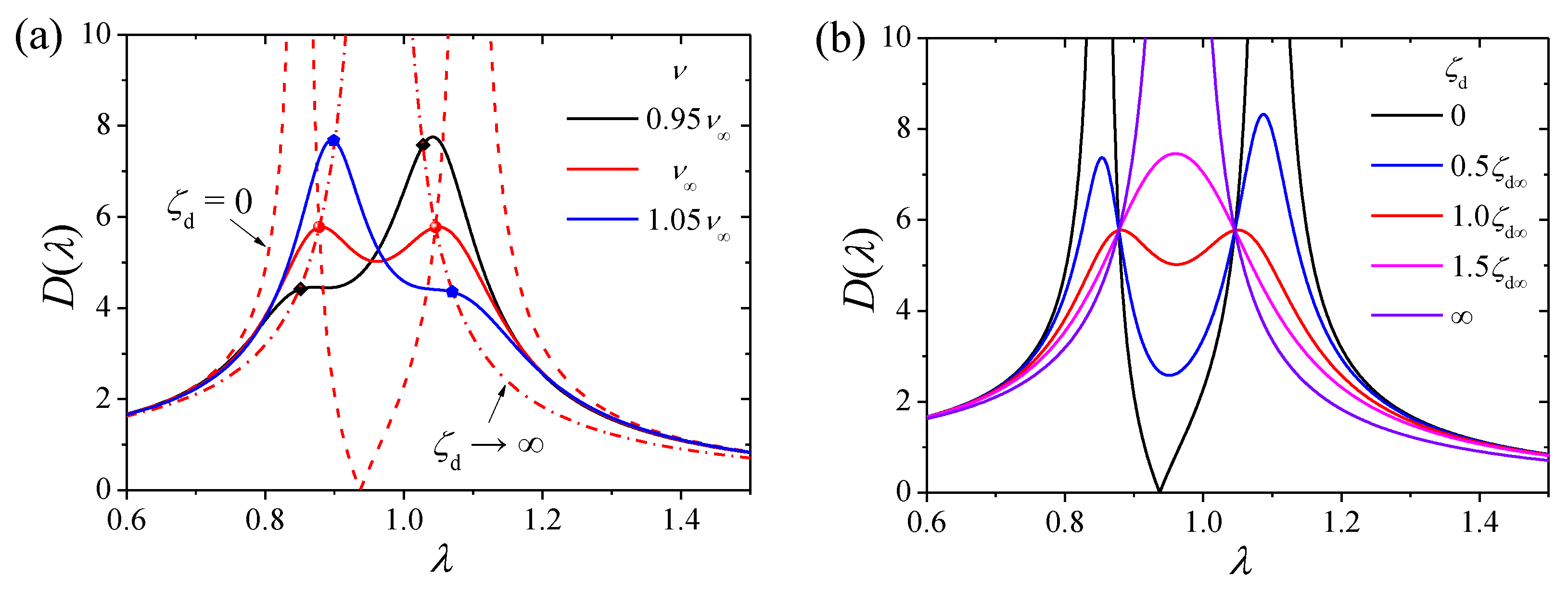
According to Den Hartog [18], the dynamic amplification function (DAF) D(λ) is defined as the modulus of H(iω), particularly ignoring ζn, as shown in Equation (8), where λ = ω/ωn is the normalized frequency. The polynomials A1(λ), A2(λ), B1(λ), and B2(λ) are determined by substituting Equation (7) into Equation (8), as shown in Equation (9). In the Equation, , , , . For TMDI and VTMDI, the coefficients are shown in Table 2.
Based on the FPA, for a determined tuning frequency ratio ν, D(λ) always passes through two fixed points, as shown in Figure 2a. The horizontal coordinates of the fixed points λ1,2 can be solved by letting ζd be 0 and infinity, i.e., . At the optimal tuning frequency ratio ν∞, the DAF values of the two fixed points are equal, i.e., D(λ1) = D(λ2) = Dopt. Consequently, we obtain the following equation:
By substituting Equation (9) into Equation (10), ν∞ can be obtained by solving Equation (11) analytically. The coordinates of the optimal fixed points (λ1, 2, Dopt) are given by Equation (12).
According to FPA, the optimal tuning damping ratio ζd∞ can be determined by assigning the fixed points to the peaks of the DAF, i.e., , as shown in Figure 2b. Based on the quotient rule of derivation, the following equation may be obtained:
Thus, the optimal tuning damping ratio ζd∞1,2, corresponding to the fixed points at λ1 and λ2, are given by Equation (14).
Considering the two fixed points, the optimal tuning damping ratio ζd∞ is taken as . Substituting Equations (9) and (12) into Equation (14), ζd∞ is analytically obtained, as shown in Equation (15).
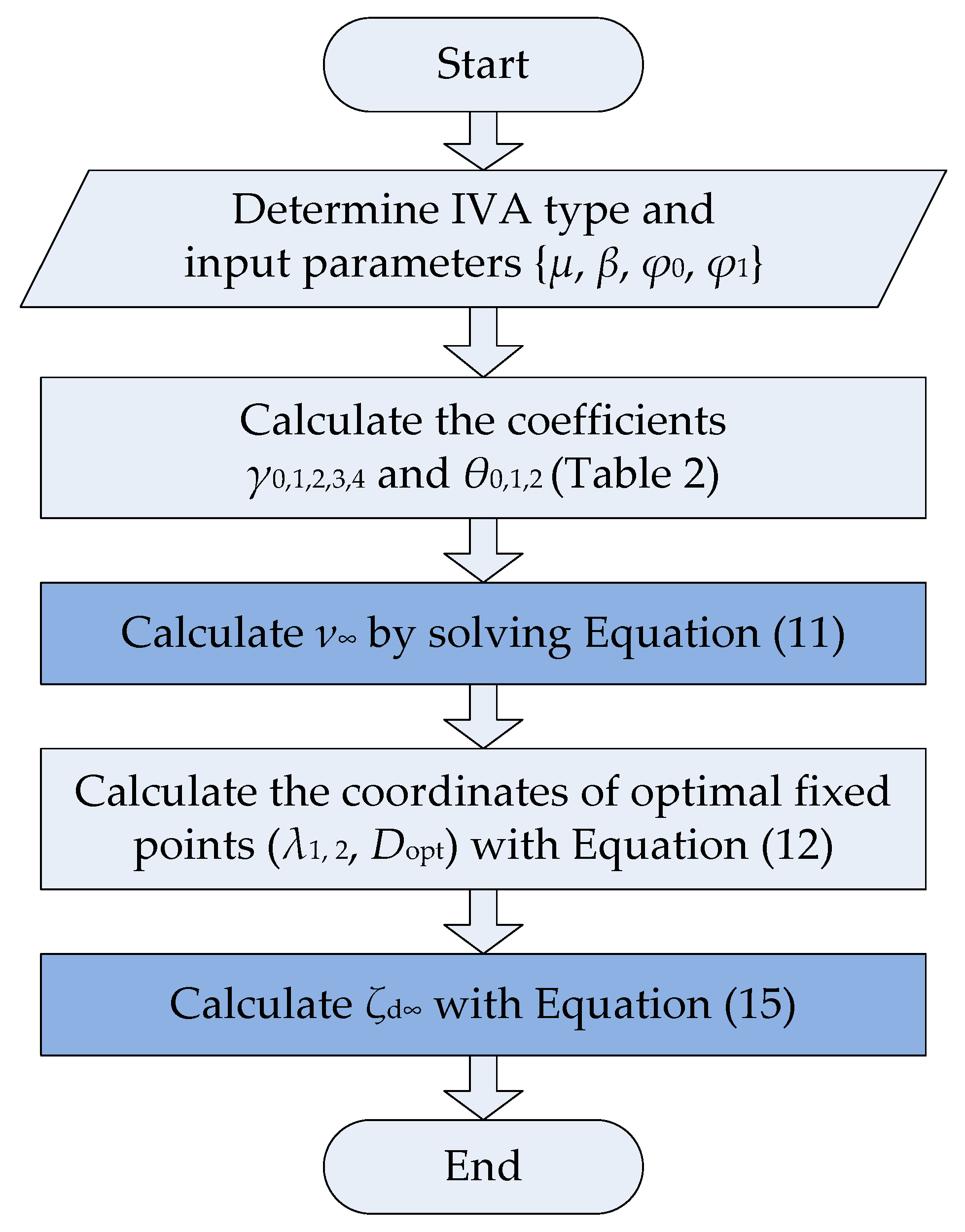
The flow chart for determining the analytical optimal parameters via FPA is summarized in Figure 3. Based on the procedure, the analytical solutions to the optimal parameters {ν∞, ζd∞} for various IVAs are obtained, as shown in Table 3. As the solution of a general VTMDI is complex, it is given in Appendix A.
It is noted that there are many optimization goals of the DVAs, such as the H∞ optimization, which aims at minimizing the maximum of the DAF. The H2 optimization is targeted for minimizing the frequency domain integration, which corresponds to the variance of the response based on the stochastic vibration theory. In the presented paper, we adopted the FPA for an H∞ optimal solution considering the two reasons. Firstly, the optimal results of the H∞ and H2 optimization are similar for stationary stochastic vibration responses according to previous studies [29,39]. Secondly, based on the fixed-point approach, the closed form solution can be derived, providing a feasible formula for practical design.
Notice that, in the proposed analytical derivation with FPA, the results for the optimal parameters (ν∞ and ζd∞) of Equations (11), (12) and (15) are only based on the coefficients of the transfer function. No extra assumption is introduced. Therefore, the derivation can be applied for DVAs that follows a transfer function with a quadratic numerator polynomial and a quartic denominator polynomial. A linear DVA with a single DOF usually follows this characteristic. The abovementioned equations can be applied to such DVAs other than the IVAs investigated in this paper.
It is indicated that when μφ1 = 0 (i.e., absent mass μ = 0 or grounded IVA φ1 = 0), the optimal parameters of the TMDI (or VTMDI) can be formulated with an equivalent mass ratio μeq compared to the corresponding conventional TMD (or VTMD). The equivalent mass ratio μeq is formulated in Equation (16), revealing the influence of installation locations. This equivalent mass ratio approach can be extended to IVAs for approximating the optimal parameters neglecting the higher order items, as displayed in Equations (17) and (18).
3. Wind-Induced Response Estimation
With the determined IVA parameters, the estimation method of the controlled wind-induced response based on the filter approach is presented in this section, which provides a basis to the formulation of ESWL.
3.1. Filter-Based Wind Load Spectrum
As an excitation input, the wind load spectrum is important for estimating the wind-induced responses. In order to obtain a closed form solution, a filter-based model is adopted to the estimation of the wind load spectrum. It is described as an analog filter applied on white-noise. The normalized generalized wind load spectrum is written as Equation (19). In the equation, Δ(s) is a filter polynomial for wind load, and δ is a normalization factor, determined by .
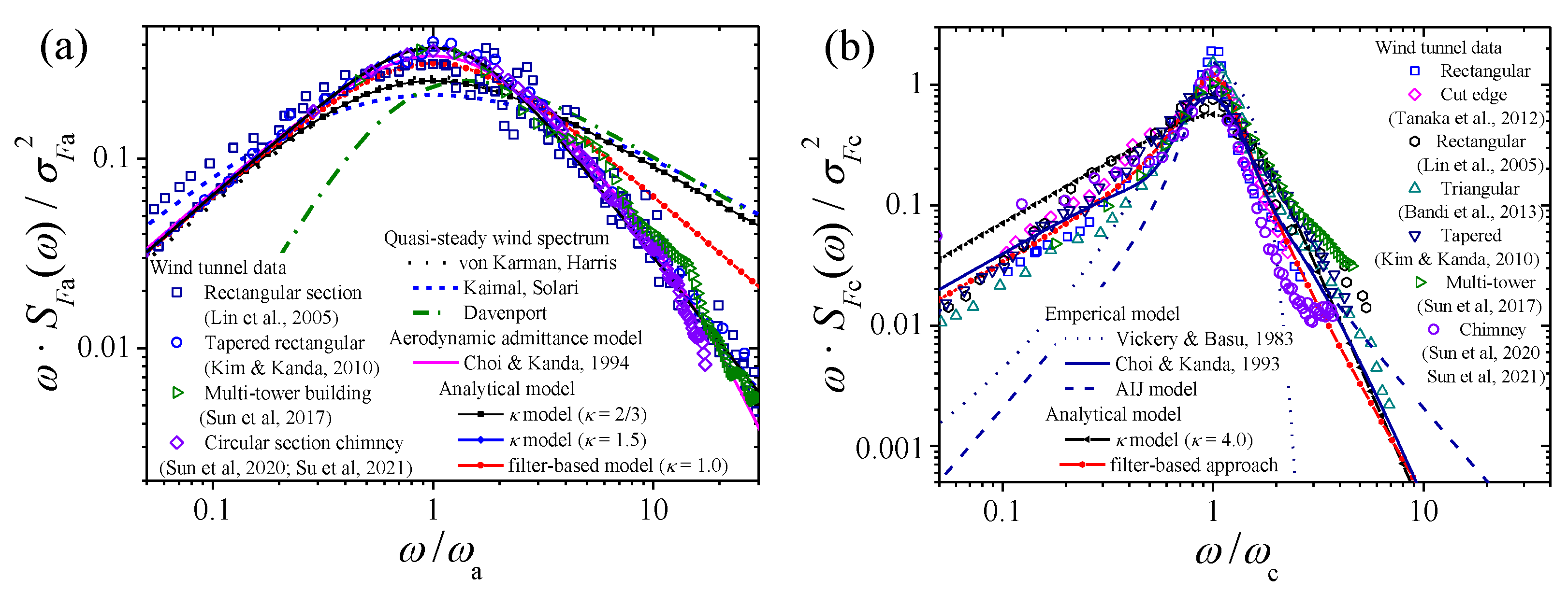
For the along-wind excitation characterized by a broad-banded spectrum, the filter polynomial is modeled by a linear function. The filter polynomial and the corresponding normalization factor are given by Equation (20). The subscript “a” stands for “along-wind”. In the model, is the characteristic frequency of the along-wind load. The model agrees well with the experimental data for tall buildings or slender structures with different configurations in literatures, as shown in Figure 4a.
The cross-wind excitation usually has a narrow-banded spectral characteristic, due to the vortex-induced turbulence. A quadratic polynomial is adopted to the model of the cross-wind spectrum, provided by Equation (21), with the subscript “c” denoting a “cross-wind”. In the equation, is a characteristic frequency of the cross-wind load, related with the vortex frequency. is the bandwidth parameter ranging from 1 to infinity. is a dissipation parameter. Note that, as the bandwidth becomes increasingly narrow, λc approaches 1. Otherwise, as λc tends to infinity, the result converges to the along-wind spectrum. This model agrees well with the experimental data for various slender structures reported in the literatures, as shown in Figure 4b.
There are many advantages for adopting the filter approach for the wind load spectra [29,42,55]. In addition to the well goodness of fit with experimental data, the major advantage of the filter approach is its simplicity in describing the physical meaning of the spectral characteristics of wind load. Moreover, it also leads to a closed form solution to the wind-induced responses, which significantly enhanced the calculation efficiency and simplicity for the analytical derivation.
3.2. Closed Form Solutions to Wind-Induced Responses Based on Filter Approach
With the filter-based wind load spectra, the dynamic wind-induced responses can be calculated through the frequency domain integral, as shown in Equation (3). With the filter approach, the frequency domain integration formatted with Equation (21) can be analytically solved [51]. In this format, the filter polynomial to the nth order is provided by , with χj (j = 0, 1, 2, …, n) being the dimensionless filter coefficients. The numerator polynomial of the even degree is less than the 2(n–1)th order, written as, , with ξj (j = 0, 1, 2, …, n–1) being the dimensionless numerator coefficients.
The solution to the integration I is expressed as two determinants of the nth order, D and N. They are calculated by Equations (A5) and (A6) (see Appendix B), respectively. D is the denominator determinant composed of filter coefficients χj. Whereas, N is the numerator determinant, similar to D, merely replacing the first row with the numerator coefficients ξj. With this approach, the closed form solutions are obtained in this section.
3.2.1. Uncontrolled Response
Substituting uncontrolled H(s) (Equation (2)), and the filter-based wind load spectral model (Equation (19)) into Equation (3), the dimensionless response (with subscript “0” representing uncontrolled) is obtained by Equation (23). The factor βd0 denotes the ratio between the dynamic response and quasi-static (also known as “background”) response.
For computing the uncontrolled along-wind and cross-wind responses, Equations (20) and (21) are substituted into Equation (23). The filter polynomial is cubic for along-wind response; meanwhile, it is quartic for the cross-wind situation. The numerator polynomial is constant, i.e., . The dimensionless filter coefficients and the integral factor are summarized in Table 4, with being the frequency ratio. The determinants N0 and D0 are calculated through Equations (A5) and (A6), as shown in Equation (24). In the equation, coefficients ψ1, ψ2, and ψ12 for along-wind and cross-wind (denoted by superscripts “a” and “c”) are given by Equations (25) and (26), respectively. Note that, for cross-wind response, the aerodynamic damping ratio ζa should be considered. Consequently, the dimensionless responses are obtained and generically described in Equation (24).
3.2.2. Controlled Response
Similarly, the controlled responses (without the subscript “0”) are calculated by Equation (27), substituting the controlled H(s) (Equation (7)) and the filter-based spectra Equation (19) into Equation (22).
The order of the filter polynomial is n = 5 for the along-wind response and n = 6 for the cross-wind response. The numerator polynomial in Equation (22) is to the 4th order, i.e., . The dimensionless coefficients and integral factor are summarized in Table 5. Comparing with Table 4 for uncontrolled responses, it is indicated that, κ = γ4κ0 for controlled responses. The dimensionless responses are obtained with the filter approach in Equation (22). The determinants N and D are calculated from Equation (A5) and (A6). Moreover, the aerodynamic damping ratio ζa should be considered in the cross-wind situation.
4. Equivalent Static Wind Load
The structural design requires ESWL to estimate the peak wind-induced responses, which may be combined with the other load effects. The basic equivalent and generalized wind force Feq targeting the top displacement of the building is formulated in Equation (28).
4.1. Gust Response Factor for Along-Wind ESWL
For along-wind ESWL, in light of the basic idea of the Davenport’s Gust Loading Factor approach [1], adopting the quasi-steady assumption that (with Iu being the turbulence intensity, and r being a modification factor), the gust response factor G may be provided by Equation (29). Furthermore, the equivalent static wind pressure peq(z) may be provided by Equation (30), where is the time-averaged wind pressure of p(z, t).
In Equation (29), βd is a factor that considers the dynamic effect. For an uncontrolled structure, it is taken as βd0 in Equation (23). While controlled with IVA, it should be calculated by Equation (27). In order to make this process explicit, a control factor is defined as the ratio between controlled βd and uncontrolled βd0, as calculated by Equation (31). In this manner, the relationship between the controlled G and the uncontrolled G0 is provided by Equation (32).
4.2. Cross-Wind ESWL
For the cross-wind response, the static response can be neglected. The wind-induced response is dominated by the dynamic component. Moreover, the quasi-steady approach is not applicable. Ignoring the mean component in Equation (28), it is obtained that . There are two approaches to estimate the ESWL.
The first one is the extended gust response factor G’, as referred to in [6], in which the mean along-wind load is used, as shown in Equation (33). The subscript “a” and “c” represent “along-wind” and “cross-wind”, respectively. Consequently, the equivalent static wind pressure in the cross-wind direction, peq,c(z), may be given by Equation (34) in proportion to the mean along-wind load .
Alternatively, another approach directly adopts the inertial load of the fundamental mode, which is expressed by Equation (35). The equivalent static wind pressure in the cross-wind direction, peq,c(z), is in proportion to the modal function Φ(z).
In either method, the cross-wind ESWL is in proportion to βd. The relationship between the controlled load peq,c and the uncontrolled load peq,c0 is provided by Equation (36). The control ratio J is estimated from Equation (32) using the cross-wind spectrum.
It is noticed that, with the proposed framework, the ESWL of the uncontrolled structure can be converted to the controlled ESWL using the control ratio J. The ratio J is dependent on the spectral parameters of the wind load and the tuning parameters of the IVA. Note that the control ratios for along-wind and cross-wind responses should be calculated separately. With this approach, it is also convenient to convert the codified ESWL for uncontrolled structures to that for the controlled structures.
5. Case Study
In this section, a numerical case study on the wind-induced vibration control and ESWL estimation of a tall chimney with IVA is performed to demonstrate the application of the proposed procedure.
The chimney is made of reinforced concrete, with a height of H = 270 m. It is assumed to be constructed in an open terrain (Type C, ASCE). The sectional dimensions along the height are listed in Table 6. The averaged outer diameter of the chimney is 25.4 m. The finite element of the chimney is established with a beam-type element. Through a modal analysis, the fundamental frequency of the chimney is calculated as ωn = 2.48 rad/s. The corresponding modal function Φ(z) is also presented in Table 6. The modal mass is M = 4588 t. The critical wind velocity of the chimney is determined as UCr = 50.2 m/s. The critical damping ratio of the chimney is ζn = 1.5%. According to the wind tunnel tests on an aeroelastic model [43], the aerodynamic damping ratio at UCr is ζa = –0.96%. In the numerical case, the most unfavorable case is considered, as the design wind velocity is equal to the critical wind velocity.
For the IVA, it is assumed that the mass ratio is μ = 1.0%, and the inertance ratio is β = 20%. The IVA is installed between z0 = 260 m (φ0 = 0.933) and z1 = 210 m (φ1 = 0.605). Using Equations (16)–(18), the optimal parameters of the IVAs are calculated, as shown in Table 7. Here, the TMDI and VTMDI cases are considered. The modulus of the frequency response functions |X(iω)/F(iω)| of uncontrolled and controlled chimney cases are shown in Figure 5. The theoretical curves (using the optimal parameters in Table 3) and the proposed ones (obtained with parameters in Table 7, obtained by Equations (17) and (18)) are compared in the figures. The results have demonstrated good agreements between the proposed formulas and the theoretical curves on the chimney case, indicating the effectiveness of the proposed optimal design method.
Based on the wind tunnel data [47,48], the wind-induced responses of the uncontrolled and controlled cases are calculated with time-history analysis. The time-history of the wind-induced top displacement responses are shown in Figure 6. The statistical results of the peak wind-induced responses are summarized in Table 8. The resulting control ratios and gust response factors obtained from the proposed ESWL framework are also shown in this table. A good agreement can be observed between the time domain method and the proposed method. The proposed method may overestimate the GRFs within a maximum relative error of 3.9% in the numerical cases, which is an acceptable error in practical engineering. Therefore, the effectiveness of the analytical framework regarding the optimal design and control performance estimation for the ESWL of structures with IVAs in this paper are illustrated.
Moreover, it can be also concluded from the wind-induced vibration control analysis results that the control ratio for VTMDI is slightly lower than that for TMDI, indicating a better control performance. However, it requires a larger stiffness and damping to maintain an optimal design state. Therefore, the designers can make a choice according to the conclusions and methods proposed in this paper. Moreover, the control ratios for cross-wind responses are lower than those for along-wind responses. This is because the cross-wind response is subjected to a more significant dynamic effect due to the vortex-induced resonance. Generally, according to the time domain analysis, with the IVA, the ESWL denoted by the gust response factors for the along-wind was reduced by approximately 15%. It reduced up to 53% for the cross-wind ESWL. The IVAs appear to be more effective to suppress the vortex-induced resonant vibration of the structures with low damping. When controlled by IVAs, the ESWL of vortex resonance become less significant, which is reduced to the along-wind ESWL, leading to an economic design for practical engineering structures.
6. Conclusions
In this paper, an analytical framework of the Equivalent Static Wind Load (ESWL) for structures with Inerter-based Vibration Absorbers (IVAs) was established. This framework includes analytical parametric optimization formulas based on the Fixed-point approach (FPA), closed form solutions for the controlled wind-induced responses based on the filter approach, and ESWL for the controlled structures based on the gust response factors.
The core of the proposed ESWL for controlled structures is based on a control ratio. It is dependent on the spectral parameters of wind load and the tuning parameters of the IVAs. A closed form solution of the control ratio is presented. With the control ratio, the original uncontrolled ESWL can be easily converted to the controlled one, which will provide a quick estimation at the preliminary design stage.
The current investigation is applicable to structures dynamically dominated by a single mode. It can be extended to more complex structures in future studies. Moreover, the presented analytical approach for IVAs is based on a general mathematical model of a transfer function with a quartic filter polynomial; it can also be applied to other DVAs with similar features, such as negative-stiffness-based DVAs, and so on.
Author Contributions
Conceptualization, N.S.; methodology, Z.C.; software, N.H.; validation, N.S., N.H. and Z.C.; formal analysis, N.S.; investigation, N.S.; resources, S.P.; data curation, Z.C.; writing—original draft preparation, N.S.; writing—review and editing, Y.U.; visualization, N.S.; supervision, Y.U.; project administration, S.P.; funding acquisition, S.P. All authors have read and agreed to the published version of the manuscript.
Funding
This research was funded by the National Key R&D Program of China (Grant No. 2022YFB2602302), National Natural Science Foundation of China (Grant Nos. 52202415, 51878129), Tianjin Science and Technology Development Project (Grant No. 22YFZCSN00030), and Tianjin Transportation Science and Technology Development Plan Project (Grant No. 2022-23).
Institutional Review Board Statement
Not applicable.
Informed Consent Statement
Not applicable.
Data Availability Statement
Not applicable.
Conflicts of Interest
The authors declare no conflict of interest.
Appendix A. Analytical Solutions of {ν∞, ζd∞} for VTMDI
In Table 3, the analytical solutions to the optimal parameters {ν∞, ζd∞} of VTMDI based on FPA are shown in Equations (A1) and (A2), where the polynomials Ψ1 and Ψ2 are shown in Equations (A3) and (A4).
Appendix B. The Determinants of D and N for Filter Approach
In Equation (22), the determinants of D and N are shown in Equations (A5) and (A6), respectively.
References
- Davenport, A.G. Gust Loading Factors. J. Struct. Div. ASCE 1967, 93, 11–34. [Google Scholar] [CrossRef]
- Simiu, E. Equivalent static wind loads for tall building design. J. Struct. Div. ASCE 1976, 102, 719–737. [Google Scholar] [CrossRef]
- Solari, G. Equivalent wind spectrum technique: Theory and applications. J. Struct. Eng. ASC 1988, 114, 1303–1323. [Google Scholar] [CrossRef]
- Kasperski, M. Extreme wind load distributions for linear and nonlinear design. Eng. Struct. 1992, 14, 27–34. [Google Scholar] [CrossRef]
- Uematsu, Y.; Yamada, M.; Karasu, A. Design wind loads for structural frames of flat long-span roofs: Gust loading factor for a structurally integrated type. J. Wind. Eng. Ind. Aerodyn. 1997, 66, 155–168. [Google Scholar] [CrossRef]
- Piccardo, G.; Solari, G. Closed form prediction of 3-D wind-excited response of slender structures. J. Wind. Eng. Ind. Aerodyn. 1998, 74–76, 697–708. [Google Scholar] [CrossRef]
- Holmes, J.D. Effective static load distributions in wind engineering. J. Wind. Eng. Ind. Aerodyn. 2002, 90, 91–109. [Google Scholar] [CrossRef]
- Kareem, A.; Zhou, Y. Gust loading factor—Past, present and future. J. Wind. Eng. Ind. Aerodyn. 2003, 91, 1301–1328. [Google Scholar] [CrossRef]
- Chen, X.Z.; Kareem, A. Equivalent static wind loads on buildings: New model. J. Struct. Eng. ASCE 2004, 130, 1425–1435. [Google Scholar] [CrossRef]
- Katsumura, A.; Tamura, Y.; Nakamura, O. Universal wind load distribution simultaneously reproducing largest load effects in all subject members on large-span cantilevered roof. J. Wind. Eng. Ind. Aerodyn. 2007, 95, 1145–1165. [Google Scholar] [CrossRef]
- Blaise, N.; Denoel, V. Principal static wind loads. J. Wind. Eng. Ind. Aerodyn. 2013, 113, 29–39. [Google Scholar] [CrossRef] [Green Version]
- Yang, Q.S.; Chen, B.; Wu, Y.; Tamura, Y. Wind-induced response and equivalent static wind load of long-span roof structures by combined Ritz-Proper Orthogonal Decomposition method. J. Struct. Eng. ASCE 2013, 139, 997–1008. [Google Scholar] [CrossRef]
- Patruno, L.; Ricci, M.; Miranda, S.D.; Ubertini, F. An efficient approach to the determination of equivalent static wind loads. J. Fluids Struct. 2017, 68, 1–14. [Google Scholar] [CrossRef]
- Su, N.; Peng, S.T.; Hong, N.N. Analyzing the background and resonant effects of wind-induced responses on large-span roofs. J. Wind. Eng. Ind. Aerodyn. 2018, 183, 114–126. [Google Scholar] [CrossRef]
- Chen, Z.Q.; Wei, C.; Li, Z.M.; Zeng, C.; Zhao, J.B.; Hong, N.N.; Su, N. Wind-induced response characteristics and equivalent static wind-resistant design method of spherical inflatable membrane structures. Buildings 2022, 12, 1611. [Google Scholar] [CrossRef]
- Kwon, D.K.; Kareem, A. Comparative study of major international wind codes and standards for wind effects on tall buildings. Eng. Struct. 2013, 51, 23–35. [Google Scholar] [CrossRef]
- Tamura, Y.; Kareem, A.; Solari, G.; Kwok, K.C.S.; Holmes, J.D.; Melbourne, W.H. Aspects of the dynamic wind-induced response of structures and codification. Wind Struct. 2005, 8, 251–268. [Google Scholar] [CrossRef]
- Den Hartog, J.P. Mechanical Vibrations, 4th ed.; Dover Publications, Inc.: McGraw-Hill, NY, USA, 1956; pp. 87–104. [Google Scholar]
- Asami, T.; Nishihara, O.; Baz, A.M. Analytical solutions to H∞ and H2 optimization of dynamic vibration absorbers attached to damped linear systems. J. Vib. Acoust. 2002, 124, 284–295. [Google Scholar] [CrossRef]
- Smith, M.C. Synthesis of mechanical networks: The Inerter. IEEE Trans. Automat. Contr. 2002, 47, 1648–1662. [Google Scholar] [CrossRef] [Green Version]
- Ikago, K.; Saito, K.; Inoue, N. Seismic control of single-degree-of-freedom structure using tuned viscous mass damper. Earthq. Eng. Struct. Dyn. 2012, 41, 453–474. [Google Scholar] [CrossRef]
- Ma, R.S.; Bi, K.M.; Hao, H. Inerter-based structural vibration control: A state-of-the-art review. Eng. Struct. 2021, 243, 112655. [Google Scholar] [CrossRef]
- Garrido, H.; Curadelli, O.; Ambrosini, D. Improvement of tuned mass damper by using rotational inertia through tuned viscous mass damper. Eng. Struct. 2013, 56, 2149–2153. [Google Scholar] [CrossRef]
- Su, N.; Peng, S.T.; Hong, N.N.; Xia, Y. Wind-induced vibration absorption using inerter-based double tuned mass dampers on slender structures. J. Build. Eng. 2022, 58, 104993. [Google Scholar] [CrossRef]
- Pietrosanti, D.; De Angelis, M.; Basili, M. Optimal design and performance evaluation of systems with tuned mass damper inerter (TMDI). Earthq. Eng. Struct. Dyn. 2017, 46, 1367–1388. [Google Scholar] [CrossRef]
- Di Matteo, A.; Masnata, C.; Pirrotta, A. Simplified analytical solution for the optimal design of Tuned Mass Damper Inerter for base isolated structures. Mech. Syst. Signal Process. 2019, 134, 106337. [Google Scholar] [CrossRef]
- Bian, J.; Zhou, X.H.; Ke, K.; Michael, C.H.Y.; Wang, Y.H. Seismic resilient steel substation with BI-TMDI: A theoretical model for optimal design. J. Constr. Steel Res. 2022, 192, 107233. [Google Scholar] [CrossRef]
- Marian, L.; Giaralis, A. Optimal design of a novel tuned mass-damper-inerter (TMDI) passive vibration control configuration for stochastically support-excited structural systems. Probabilist. Eng. Mech. 2014, 38, 156–164. [Google Scholar] [CrossRef]
- Su, N.; Xia, Y.; Peng, S.T. Filter-based inerter location dependence analysis approach of Tuned mass damper inerter (TMDI) and optimal design. Eng. Struct. 2022, 250, 113459. [Google Scholar] [CrossRef]
- Zhu, Z.W.; Lei, W.; Wang, Q.H.; Tiwari, N.D.; Hazra, B. Study on wind-induced vibration control of linked high-rise buildings by using TMDI. J. Wind. Eng. Ind. Aerodyn. 2020, 205, 104306. [Google Scholar] [CrossRef]
- Djerouni, S.; Elias, S.; Abdeddaim, M.; Rupakhety, R. Optimal design and performance assessment of multiple tuned mass damper inerters to mitigate seismic pounding of adjacent buildings. J. Build. Eng. 2022, 48, 103994. [Google Scholar] [CrossRef]
- Lazar, I.F.; Neild, S.A.; Wagg, D.J. Using an inerter-based device for structural vibration suppression. Earthq. Eng. Struct. Dyn. 2014, 43, 1129–1147. [Google Scholar] [CrossRef] [Green Version]
- Shen, W.; Niyitangamahoro, A.; Feng, Z.; Zhu, H. Tuned inerter dampers for civil structures subjected to earthquake ground motions: Optimum design and seismic performance. Eng. Struct. 2019, 198, 109470. [Google Scholar] [CrossRef]
- Ren, M.Z. A variant design of the dynamic vibration absorber. J. Sound Vib. 2001, 245, 762–770. [Google Scholar] [CrossRef]
- Cheung, Y.L.; Wong, W.O. H2 optimization of a non-traditional dynamic vibration absorber for vibration control of structures under random force excitation. J. Sound Vib. 2011, 330, 1039–1044. [Google Scholar] [CrossRef]
- Masnata, C.; Matteo, A.D.; Adam, C.; Pirrotta, A. Smart structures through nontraditional design of Tuned Mass Damper Inerter for higher control of base isolated systems. Mech. Res. Commun. 2020, 105, 103513. [Google Scholar] [CrossRef]
- Alotta, G.; Failla, G. Improved inerter-based vibration absorbers. Int. J. Mech. Sci. 2021, 192, 106087. [Google Scholar] [CrossRef]
- Zhang, R.F.; Zhao, Z.P.; Pan, C.; Ikago, K.; Xue, S.T. Damping enhancement principle of inerter system. Struct. Control Health Monit. 2020, 27, e2523. [Google Scholar] [CrossRef]
- Su, N.; Bian, J.; Peng, S.T.; Xia, Y. Generic optimal design approach for inerter-based tuned mass systems. Int. J. Mech. Sci. 2022, 233, 113459. [Google Scholar] [CrossRef]
- Zhang, M.J.; Xu, F.Y. Tuned mass damper for self-excited vibration control: Optimization involving nonlinear aeroelastic effect. J. Wind. Eng. Ind. Aerodyn. 2022, 220, 104836. [Google Scholar] [CrossRef]
- Yu, H.Y.; Zhang, M.J.; Hu, G. Effect of inerter locations on the vibration control performance of nonlinear energy sink inerter. Eng. Struct. 2022, 273, 115121. [Google Scholar] [CrossRef]
- Spanos, P.D.; Sun, Y.; Su, N. Advantages of filter approaches for the determination of wind-induced response of large-span roof structures. J. Eng. Mech. ASCE 2017, 143, 04017066. [Google Scholar] [CrossRef]
- Wang, Z.; Giaralis, A. Enhanced motion control performance of the tuned mass damper inerter through primary structure shaping. Struct. Control Health Monit. 2021, 28, e2756. [Google Scholar] [CrossRef]
- Su, N.; Bian, J.; Peng, S.T.; Xia, Y. Impulsive resistant optimization design of tuned viscous mass damper (TVMD) based on stability maximization. Int. J. Mech. Sci. 2023, 239, 107876. [Google Scholar] [CrossRef]
- Lin, N.; Letchford, C.; Tamura, Y.; Liang, B.; Nakamura, O. Characteristics of wind forces acting on tall buildings. J. Wind. Eng. Ind. Aerodyn. 2005, 93, 217–242. [Google Scholar] [CrossRef]
- Kim, Y.C.; Kanda, J. Characteristics of aerodynamic forces and pressures on square plan buildings with height variations. J. Wind. Eng. Ind. Aerodyn. 2010, 98, 449–465. [Google Scholar] [CrossRef]
- Sun, Y.; Li, Z.Y.; Sun, X.Y.; Su, N.; Peng, S.T. Interference effects between two tall chimneys on wind loads and dynamic responses. J. Wind. Eng. Ind. Aerodyn. 2020, 206, 104227. [Google Scholar] [CrossRef]
- Su, N.; Li, Z.Y.; Peng, S.T.; Uematsu, Y. Interference effects on aeroelastic responses and design wind loads of twin high-rise reinforced concrete chimneys. Eng. Struct. 2021, 233, 111925. [Google Scholar] [CrossRef]
- Sun, X.Y.; Liu, H.; Su, N.; Wu, Y. Investigation on Wind Tunnel Tests of the Kilometer Skyscraper. Eng. Struct. 2021, 148, 340–356. [Google Scholar] [CrossRef]
- Choi, H.; Kanda, J. Semi-empirical formulae for dynamic alongwind force estimation. J. Struct. Constr. Eng. (Trans. AIJ) 1994, 463, 9–18. [Google Scholar] [CrossRef]
- Tanaka, H.; Tamura, Y.; Ohtake, K.; Nakai, M.; Kim, Y.C. Experimental investigation of aerodynamic forces and wind pressures acting on tall buildings with various unconventional configurations. J. Wind. Eng. Ind. Aerodyn. 2012, 107–108, 179–191. [Google Scholar] [CrossRef]
- Bandi, E.K.; Tamura, Y.; Yoshida, A.; Kim, Y.C.; Yang, Q. Experimental investigation on aerodynamic characteristics of various triangular-section high-rise buildings. J. Wind. Eng. Ind. Aerodyn. 2013, 122, 60–68. [Google Scholar] [CrossRef]
- Vickery, B.J.; Basu, R. Simplified approaches to the evaluation of the across-wind response of chimneys. J. Wind. Eng. Ind. Aerodyn. 1983, 14, 153–166. [Google Scholar] [CrossRef]
- Choi, H.; Kanda, J. Proposed formulae for the power spectral densities of fluctuating lift and torque on rectangular 3-D cylinders. J. Wind. Eng. Ind. Aerodyn. 1993, 46–47, 507–516. [Google Scholar] [CrossRef]
- Su, N.; Peng, S.T.; Hong, N.N. Universal simplified spectral models and closed form solutions to the wind-induced responses for high-rise structures. Results Eng. 2021, 10, 100230. [Google Scholar] [CrossRef]
Figure 1.
A generalized SDOF system coupling with an IVA of various configurations.

Figure 2.
The DAF curves D(λ) with different ν and ζd. (a) D(λ) with different ν; the fixed points are equal when ν = ν∞. (b) D(λ) at ν∞ with different ζd; the fixed points are approximately assigned to the equal peaks when ζd = ζd∞.
Figure 2.
The DAF curves D(λ) with different ν and ζd. (a) D(λ) with different ν; the fixed points are equal when ν = ν∞. (b) D(λ) at ν∞ with different ζd; the fixed points are approximately assigned to the equal peaks when ζd = ζd∞.

Figure 3.
A flow chart for determining the analytical optimal parameters via FPA (the procedures that output optimal parameters are highlighted).
Figure 3.
A flow chart for determining the analytical optimal parameters via FPA (the procedures that output optimal parameters are highlighted).

Figure 4.
Comparison between the spectral model and experimental data reported in relevant literatures [45,46,47,48,49,50,51,52,53,54,55]. (a) along-wind; (b) cross-wind.

Figure 5.
The modulus of frequency response functions |X(iω)/F(iω)| of uncontrolled and controlled chimney cases. (a) TMDI. (b) VTMDI.
Figure 5.
The modulus of frequency response functions |X(iω)/F(iω)| of uncontrolled and controlled chimney cases. (a) TMDI. (b) VTMDI.

Figure 6.
The time-history of wind-induced top displacement responses of uncontrolled and controlled chimney cases. (a) Along-wind. (b) Cross-wind.
Figure 6.
The time-history of wind-induced top displacement responses of uncontrolled and controlled chimney cases. (a) Along-wind. (b) Cross-wind.


Table 1.
Definitions of the tuning parameters of the IVA.
| Tuning Parameter | Symbol | Definition |
|---|---|---|
| Tuning mass ratio | μ | m/M |
| Tuning inertance ratio | β | b/M |
| Nominal frequency | ωd | |
| Nominal damping ratio | ν | |
| Tuning frequency ratio | ζd | ωd/ωn |
Table 2.
Dimensionless coefficients of the normalized transfer function H(s) for TMDI and VTMDI.
| Coefficient | TMDI | VTMDI |
|---|---|---|
| γ0 | ||
| γ1 | ||
| γ2 | ||
| γ3 | ||
| γ4 | ||
| θ0 | ||
| θ1 | ||
| θ2 | 1 | 1 |
Table 3.
Analytical solutions to the optimal parameters {ν∞, ζd∞} of various IVAs obtained based on FPA.
Table 3.
Analytical solutions to the optimal parameters {ν∞, ζd∞} of various IVAs obtained based on FPA.
| IVA | Parameter | ν∞ | ζd∞ |
|---|---|---|---|
| TMD [18,19] | β = 0, φ0 = 1, φ1 = 0 | ||
| TMDI [28,39] | Arbitrary {μ, β, φ0, φ1} | ||
| TMDI | μφ1 = 0 (TID [32,33], or grounded TMDI [25,26,27]) | ||
| VTMD [34,35] | β = 0, φ0 = 1, φ1 = 0 | ||
| VTMDI [28,39] | Arbitrary {μ, β, φ0, φ1} | Equation (A1) | Equation (A2) |
| VTMDI | φ1 = 0 (grounded VTMDI [36]) | ||
| VTMDI | μ = 0 (TVMD [21], TID2 [37], or VTID [39]) | ||
| VTMDI | μφ1 = 0 |
Table 4.
Dimensionless filter coefficients for the uncontrolled wind-induced responses.
| Coefficient | Along-Wind | Cross-Wind |
|---|---|---|
| χ0 | 1 | |
| χ1 | ||
| χ2 | ||
| χ3 | ||
| χ4 | — | |
| ξ0 | 1 | 1 |
| κ0 | 1 |
Table 5.
Dimensionless filter coefficients for the controlled wind-induced responses.
| Coefficient | Along-Wind | Cross-Wind |
|---|---|---|
| χ0 | ||
| χ1 | ||
| χ2 | ||
| χ3 | ||
| χ4 | ||
| χ5 | ||
| χ6 | — | |
| ξ0 | ||
| ξ1 | ||
| ξ2 | ||
| κ |
Table 6.
Geometric profile and modal function of the chimney.
| Height (m) | Outer Diameter (m) | Thickness (m) | Modal Function Φ(z) |
|---|---|---|---|
| 270 | 16.9 | 0.45 | 1.000 |
| 260 | 17.3 | 0.45 | 0.933 |
| 250 | 17.7 | 0.45 | 0.866 |
| 240 | 18.1 | 0.50 | 0.799 |
| 230 | 18.5 | 0.50 | 0.733 |
| 220 | 18.9 | 0.50 | 0.668 |
| 210 | 19.3 | 0.50 | 0.605 |
| 200 | 19.7 | 0.55 | 0.543 |
| 180 | 20.5 | 0.55 | 0.429 |
| 160 | 22.1 | 0.60 | 0.328 |
| 140 | 23.7 | 0.65 | 0.240 |
| 120 | 25.3 | 0.65 | 0.168 |
| 100 | 26.9 | 0.70 | 0.110 |
| 80 | 28.9 | 0.80 | 0.066 |
| 40 | 33.7 | 0.90 | 0.015 |
| 0 | 38.5 | 1.00 | 0.000 |
Table 7.
Determined IVA parameters for the chimney case.
| Parameter | TMDI | VTMDI |
|---|---|---|
| μeq (%) | 3.15 | 3.15 |
| νopt | 0.969 | 1.016 |
| ζdopt (%) | 10.71 | 10.96 |
| m (ton) | 45.88 | 45.88 |
| c (kN·s/m) | 496 | 532 |
| k (kN/m) | 5569 | 6119 |
| b (kN·s2/m) | 917.6 | 917.6 |
Table 8.
Peak wind-induced responses, control ratios, and gust response factors for the cases.
| Direction | Parameter | Uncontrolled | TMDI | VTMDI |
|---|---|---|---|---|
| Along-wind | Top displacement (m) | 0.245 | 0.207 | 0.206 |
| Base shear force (MN) | 17.72 | 15.50 | 15.46 | |
| Base bending moment (GN·m) | 2.793 | 2.388 | 2.381 | |
| Control ratio J (time domain method) | — | 0.676 | 0.670 | |
| Gust Response Factor G (time domain method) | 1.93 | 1.63 | 1.62 | |
| Control ratio J (proposed method) | — | 0.692 | 0.680 | |
| Gust Response Factor G (proposed method) | 1.95 | 1.66 | 1.64 | |
| Cross-wind | Top displacement (m) | 0.422 | 0.197 | 0.194 |
| Base shear force (MN) | 19.36 | 9.14 | 8.95 | |
| Base bending moment (GN·m) | 4.033 | 1.901 | 1.868 | |
| Control ratio J (time domain method) | — | 0.467 | 0.461 | |
| Gust Response Factor G’ (time domain method) | 3.32 | 1.55 | 1.53 | |
| Control ratio J (proposed method) | — | 0.476 | 0.469 | |
| Gust Response Factor G’ (proposed method) | 3.38 | 1.61 | 1.59 |
Publisher’s Note: MDPI stays neutral with regard to jurisdictional claims in published maps and institutional affiliations. |
© 2022 by the authors. Licensee MDPI, Basel, Switzerland. This article is an open access article distributed under the terms and conditions of the Creative Commons Attribution (CC BY) license (https://creativecommons.org/licenses/by/4.0/).
Share and Cite
MDPI and ACS Style
Su, N.; Peng, S.; Chen, Z.; Hong, N.; Uematsu, Y. Equivalent Static Wind Load for Structures with Inerter-Based Vibration Absorbers. Wind 2022, 2, 766-783. https://doi.org/10.3390/wind2040040
AMA Style
Su N, Peng S, Chen Z, Hong N, Uematsu Y. Equivalent Static Wind Load for Structures with Inerter-Based Vibration Absorbers. Wind. 2022; 2(4):766-783. https://doi.org/10.3390/wind2040040
Chicago/Turabian StyleSu, Ning, Shitao Peng, Zhaoqing Chen, Ningning Hong, and Yasushi Uematsu. 2022. "Equivalent Static Wind Load for Structures with Inerter-Based Vibration Absorbers" Wind 2, no. 4: 766-783. https://doi.org/10.3390/wind2040040