Aquatic Plant Dynamics in Lowland River Networks: Connectivity, Management and Climate Change

Abstract

The spatial structure and evolution of river networks offer tremendous opportunities to study the processes underlying metacommunity patterns in the wild. Here we explore several fundamental aspects of aquatic plant biogeography. How stable is plant composition over time? How similar is it along rivers? How fast is the species turnover? How does that and spatial structure affect our species richness estimates across scales? How do climate change, river management practices and connectivity affect species composition and community structure? We answer these questions by testing twelve hypotheses and combining two spatial surveys across entire networks, a long term temporal survey (21 consecutive years), a trait database, and a selection of environmental variables. From our river reach scale survey in lowland rivers, hydrophytes and marginal plants (helophytes) showed contrasting patterns in species abundance, richness and autocorrelation both in time and space. Since patterns in marginal plants reflect at least partly a sampling artefact (edge effect), the rest of the study focused on hydrophytes. Seasonal variability over two years and positive temporal autocorrelation at short time lags confirmed the relatively high regeneration abilities of aquatic plants in lowland rivers. Yet, from 1978 to 1998, plant composition changed quite dramatically and diversity decreased substantially. The annual species turnover was relatively high (20%–40%) and cumulated species richness was on average 23% and 34% higher over three and five years respectively, than annual survey. The long term changes were correlated to changes in climate (decreasing winter ice scouring, increasing summer low flows) and management (riparian shading). Over 21 years, there was a general erosion of species attributes over time attributed to a decrease in winter ice scouring, increase in shading and summer low flows, as well as a remaining effect of time which may be due to an erosion of the regional species pool. Temporal and spatial autocorrelation analyses indicated that long term hydrophyte biomonitoring, for the Water Framework Directive in lowland rivers, may be carried out at 4–6 years intervals for every 10 km of rivers. From multi-scale and abundance-range size analyses evidence of spatial isolation and longitudinal connectivity was detected, with no evidence of stronger longitudinal connectivity (fish and water current propagules dispersal) than spatial isolation (bird, wind and human dispersal) contrary to previous studies. The evidence for longitudinal connectivity was rather weak, perhaps resulting from the effect of small weirs. Further studies will need to integrate other aquatic habitats along rivers (regional species pool) and larger scales to increase the number of species and integrate phylogeny to build a more eco-evolutionary approach. More mechanistic approaches will be necessary to make predictions against our changing climate and management practices.

1. Introduction

The study of species distribution (biogeography) has long fascinated scholars of natural history and geology [1,2]. Darwin subsequently offered a mechanistic explanation [3] (pp. 318–319): immigration of individuals from a species’ (individuals’) pool controlled by dispersal barriers and descent with modification regulated through natural selection, competition for resources being the most important pressure. He attributed the wide distribution of freshwater organisms to favourable means of dispersal (pp. 323–330, 343–347) and lessened competition (p. 346) in aquatic habitats. Warming [4] (pp. 150–156) gave the first comprehensive outline on the importance of plant form, overwintering, and vegetative reproduction and dispersal in aquatic plant communities.

The role of connectivity in spatially structured environments is still at the core of landscape ecology, metapopulation and metacommunity theories [5,6,7]. Connectivity is a function of species migration rates relative to patch sizes and dispersal kernel scaling the effect of distance on migration rates [6]. In metacommunities, species diversity tends to peak at intermediate dispersal rates [8,9,10].

The spatial structure and evolution of river networks offer tremendous opportunities to study the processes underlying metacommunity patterns in the wild. At large spatio-temporal scales, glaciation cycles, river capture and natural barriers can have profound effects on species distribution, speciation and diversity [11,12,13,14,15,16,17,18], and similarly at smaller spatio-temporal scales with artificial barriers such as dams and small weirs [19,20,21,22,23].

The dynamics of plants is perhaps most visible at fine scale in rivers where a mosaic of plant species, sand and gravel is in perpetual movement under the effects of vegetative growth and die-back and the force of water current [24]. Aquatic plant propagules drift along the water current, take animal lifts and hide in sediments to reappear at a later stage [3,25,26,27,28]. Direct measurements of individual species dispersal in a metacommunity (here aquatic plants) are, however, prohibitive at the scale of a whole river network. Current theoretical predictions of species richness and turnover use neutral theory whose key limiting assumption is that all individuals, regardless of species, share the same set of traits [7,29]. In contrast, empirical approaches use the existing diversity of species traits and a qualitative theoretical framework (e.g., habitat templet) to make predictions in co-occurrence of trait modalities (attributes) and local resources [30,31,32,33,34]. Local resources filter out species from the species pool and contribute determining large scale plant zonation and river types [35,36]. Both disturbance and spatial heterogeneity of resources shape patterns of plant distribution and diversity along and across rivers [31,37] as well as the directionality of river flows within an entire network [38,39,40].

Some interesting empirical inferences have been made in river network macro-ecological studies using plants’ intrinsic properties. Notably, Riis and Sand-Jensen [41] used species range-abundance patterns to infer higher dispersal rates along rivers than between rivers, and a stronger response from the amphibious species (helophytes) relative to strictly submerged species (hydrophytes), as suggested from metapopulation theory. They interpreted departure from expectations (high abundance of rare species of hydrophytes) to historical causes (local relict of former species pool, [42]). Using a different approach, Demars and Harper [43] showed that both resources (depth, substrate) and the spatial structure of the river network (river basin isolation and longitudinal connectivity) explained the distribution of hydrophytes in lowland calcareous rivers. Plant dispersal and regeneration abilities explained the impact of river spatial structure on plant distribution, supported by other findings from more detailed local studies in other lowland rivers [25,26,27,28,44,45,46,47,48,49,50,51,52,53].

Some of these interesting inferences hinge however on the definition of aquatic plants, as strict hydrophytes may not disperse in the same way as amphibious or helophytes [41]. If species diversity is only weakly sensitive to reach area in rivers beyond 50 m length survey [54,55], the richness and abundance of marginal plants (mostly helophytes) relative to strict hydrophytes (mostly submerged plants) are probably not comparable, especially along the river course as the channel area increases relative to marginal length surveyed (edge effect). Differences in river bank structure also alter the relative diversity of marginal species [56]. This sampling artefact (edge effect) might explain why mean local abundance of hydrophytes greatly exceeded marginal species in Riis and Sand-Jensen [41], a point the authors did not discuss, but which could bias their results and interpretations. Moreover, and surprisingly, Riis and Sand-Jensen [41] did not test statistically (or appropriately) their findings. In his community structure analyses, Demars [57] used abundance data based on the non-linear Braun-Blanquet scale despite a recommendation by Wiegleb [54,58] to use percentage cover (or linear scale). Hence, the findings of Demars [57] may be biased as well. Other artefacts have been suggested such as the mid-domain effect along rivers [59]. Since species diversity and abundance are at the heart of community structure analyses, more rigour in data analyses is required.

Substantial annual species turnover in rivers draining arid land indicated the need to survey rivers temporally to estimate accurately species richness [37]. In lowland European rivers, annual turnover is seldom reported, and a 10 year study indicated small stochastic annual changes in plant composition [60]. Similarly, in a spatial context, it is still not known whether the observed low species richness in individual headwaters (e.g., [61]) translates into overall low species richness across headwaters of a river network, see [62]. Species richness is thus intimately related to species turnover. Whether species turnover is high enough to alter species assemblages can be deduced from autocorrelation analyses [63]. Yet, autocorrelation analyses of aquatic plants in streams have only been run for individual species or community structure indices rather than species composition e.g., [55,64], with the exception of the streams of the Rhine floodplain to demonstrate independence of sites [65]. In natural river networks, local resources (depth, substrate) tend to be correlated to distance from source of the river, and thus may prevent spatial effects from being disentangled from environmental effects [66]. Species richness tends to be mostly dependent on the distribution of common species [67] and common species tend to be the dominant species [41]. Hence analyses and modelling of species rank-abundance and abundance-occurrence patterns in time across replicated sites or in space in river networks may help to infer processes shaping species richness.

This study looks through fundamental and complementary properties of species pattern analyses to infer underlying processes of community assembly. These fundamental properties are spatio-temporal structure (connectivity), endogenous factors (species properties), exogenous factors (disturbance, resources), predictability, sampling artefacts (edge effect) and scales of observation in time and space. Taken together they will allow basic ecological questions to be better addressed, which in turn will help assess aquatic ecosystem health. How stable (autocorrelated) is plant composition over time? How similar (autocorrelated) is it along rivers? How fast is the species turnover? How does that and spatial structure affect our species richness estimates across scales? What does drive observed changes in plant patterns: spatio-temporal structure, exogenous or endogenous factors? Are these changes predictable (deterministic, stochastic or artefactual)? How do climate change, river management practices and connectivity affect species composition and community structure?

We test this general approach using the trait database and attribute groups of Willby et al. [68] and revisit three complementary datasets: (1) monthly aquatic plant surveys for two years and every summer for 21 consecutive years at six sites along two rivers [54,60,69]; (2) one-off survey of 62 sites, with a subset resurveyed annually over three years, in the lowland rivers of Norfolk where the effects of spatial connectivity and exogenous factors were disentangled [43]; and (3) one-off survey of 44 sites in the Welland river network where indicator species richness was shown to increase with distance from source [61].

We also formulated a set of key hypotheses (H) based on temporal, spatial and cross scale patterns in species composition (H1-4) and structure (H5-7), reflecting a priori exogenous (H8) and endogenous (H9-12) underlying processes:

(1)

Within year temporal changes in species composition will generate the highest positive autocorrelation with short time lags (less than three months) and 12 months intervals, and possible negative autocorrelation at six months intervals due to differences in life cycle of hydrophytes [54,70];

(2)

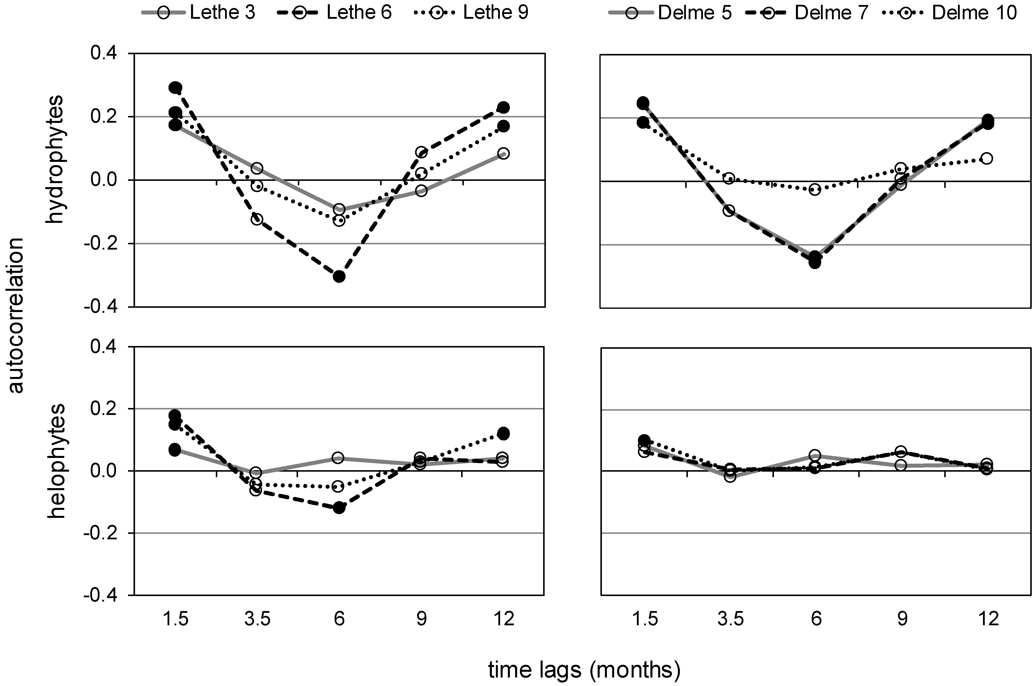
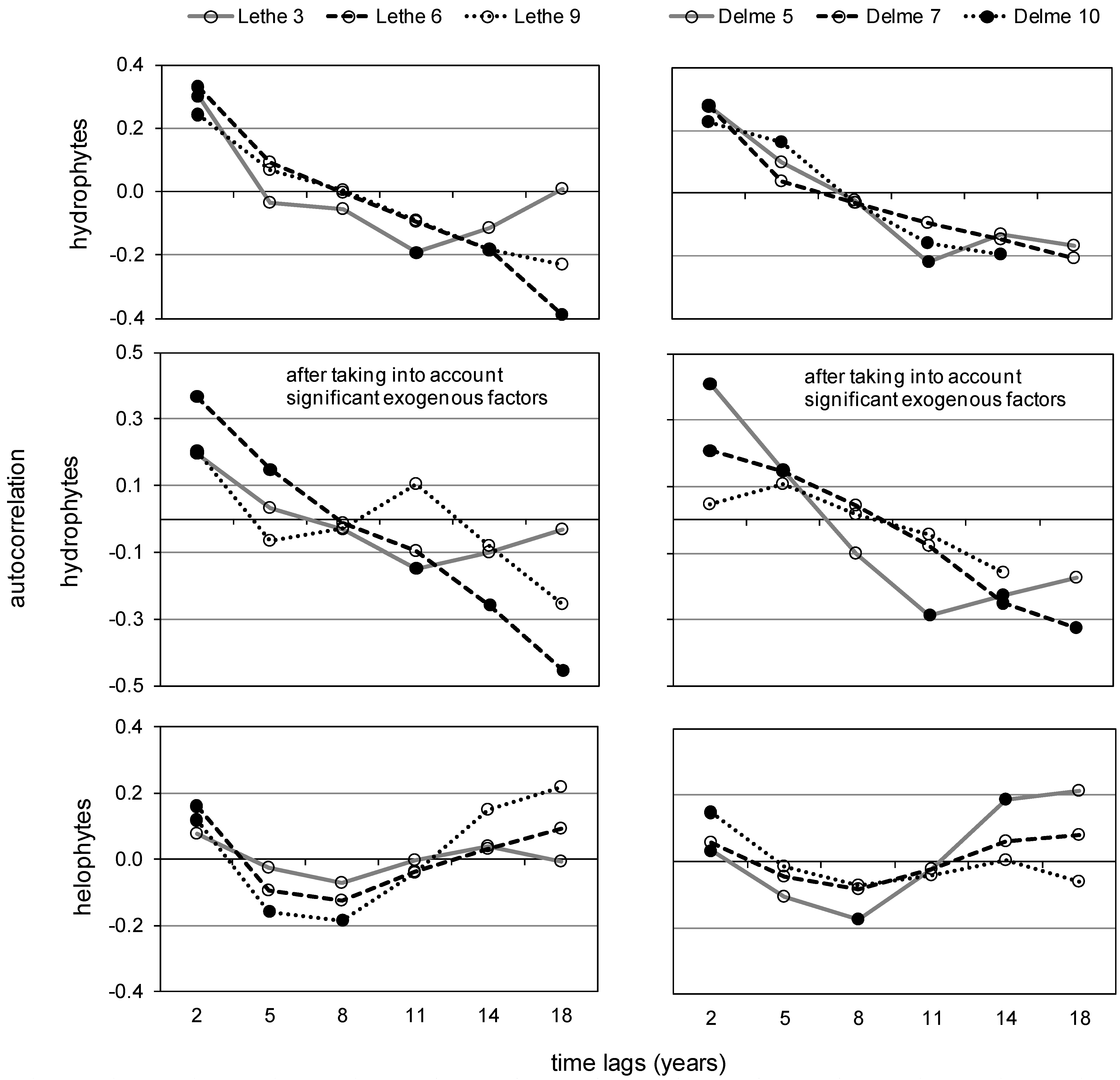
Yearly autocorrelation in species composition will decrease over time, but will stay positive in the absence of changes in the dynamics of exogenous factors (underlying deterministic gradient). Temporal negative autocorrelation would have to result from “catastrophic” changes (shift in dominant species)—unexpected here [60];

(3)

At short space intervals (km), spatial autocorrelation along the main river channel will be positive and higher than across an entire river network due to dispersal limitation across rivers, directionality of flow along rivers and regeneration abilities of hydrophytes [41,43];

(4)

At longer spatial intervals (tens of km) along the main stem, autocorrelation will decrease and possibly become negative due to differences in local resources creating river zonation. Trends in spatial autocorrelation of species composition after taking into account local resources will be weaker, but more reliably linked to plant dispersal abilities [43];

(5)

Richness, cover, diversity, evenness and abundance patterns will fluctuate slightly around a mean value over time (in years) in the absence of changes in the dynamics of exogenous factors [60];

(6)

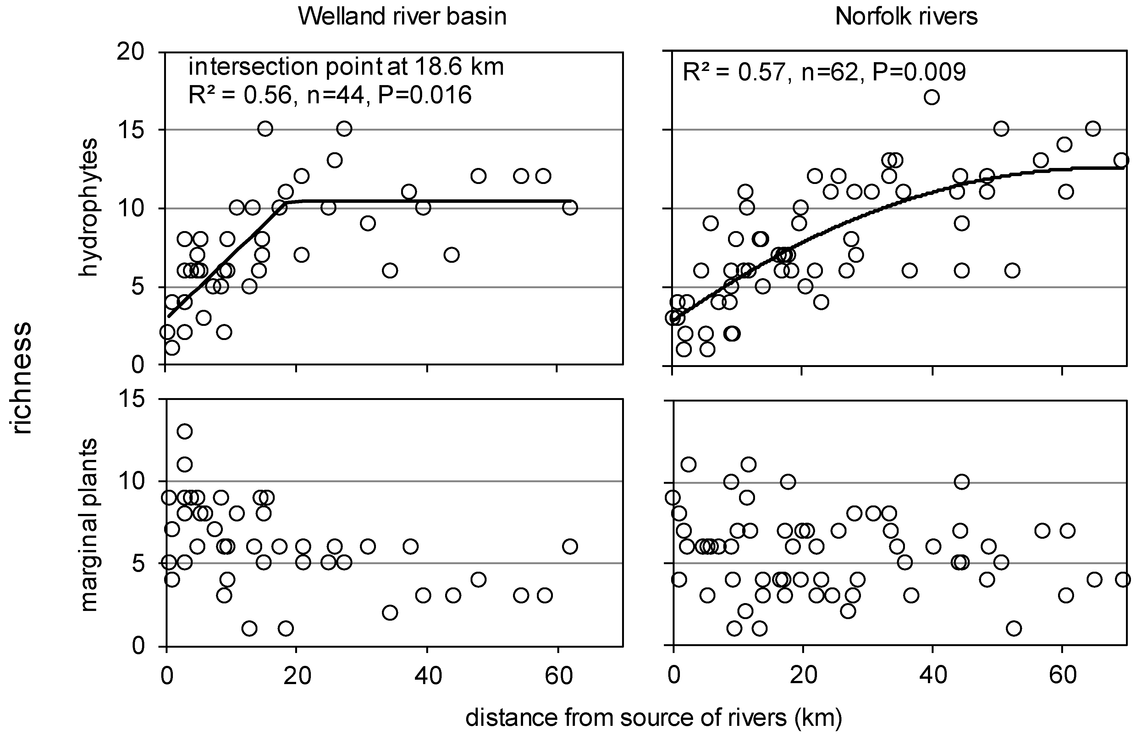
Species richness increases along individual rivers for strict hydrophytes but not for marginal plants due to a sampling artefact (edge effect);

(7)

With richness increasing along rivers (species packing), we expect an increase in evenness and species trait diversity (i.e., attribute groups, sensu Willby et al. [68]);

(8)

If biotic gradients (change with time or distance in species composition and community structure) are observed, deterministic exogenous factors can explain them, such as change in climate (changes in magnitude, timing and frequency of high and low flow events, ice scouring, high temperature), management practices (weed cutting, riparian maintenance), biotic competitors (cover of green algae), depth and substrate;

(9)

Significant exogenous factors are related to expected species attributes based on a priori expectations [31,43,65,68];

(10)

Annual species richness will be similar when quantified over one, three or five years, assuming an expected low species turnover in those lowland rivers with oceanic climate [43,60];

(11)

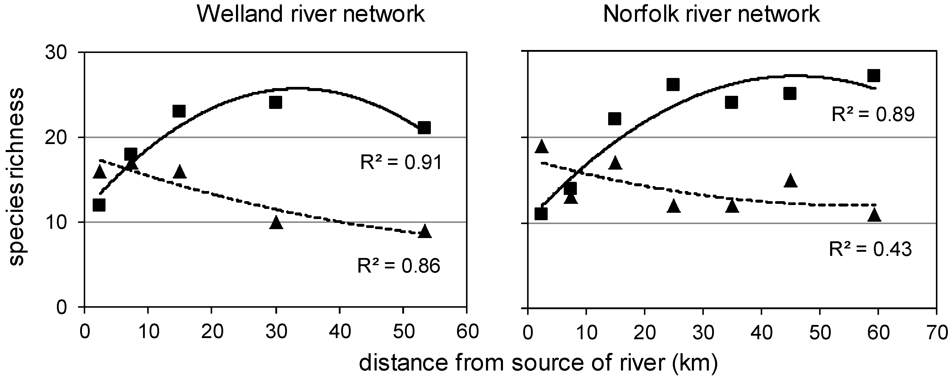
The increase in hydrophyte richness with distance from source will be less pronounced at network scale than at individual site scale due to dispersal constraints (isolation), especially in the headwaters [62];

(12)

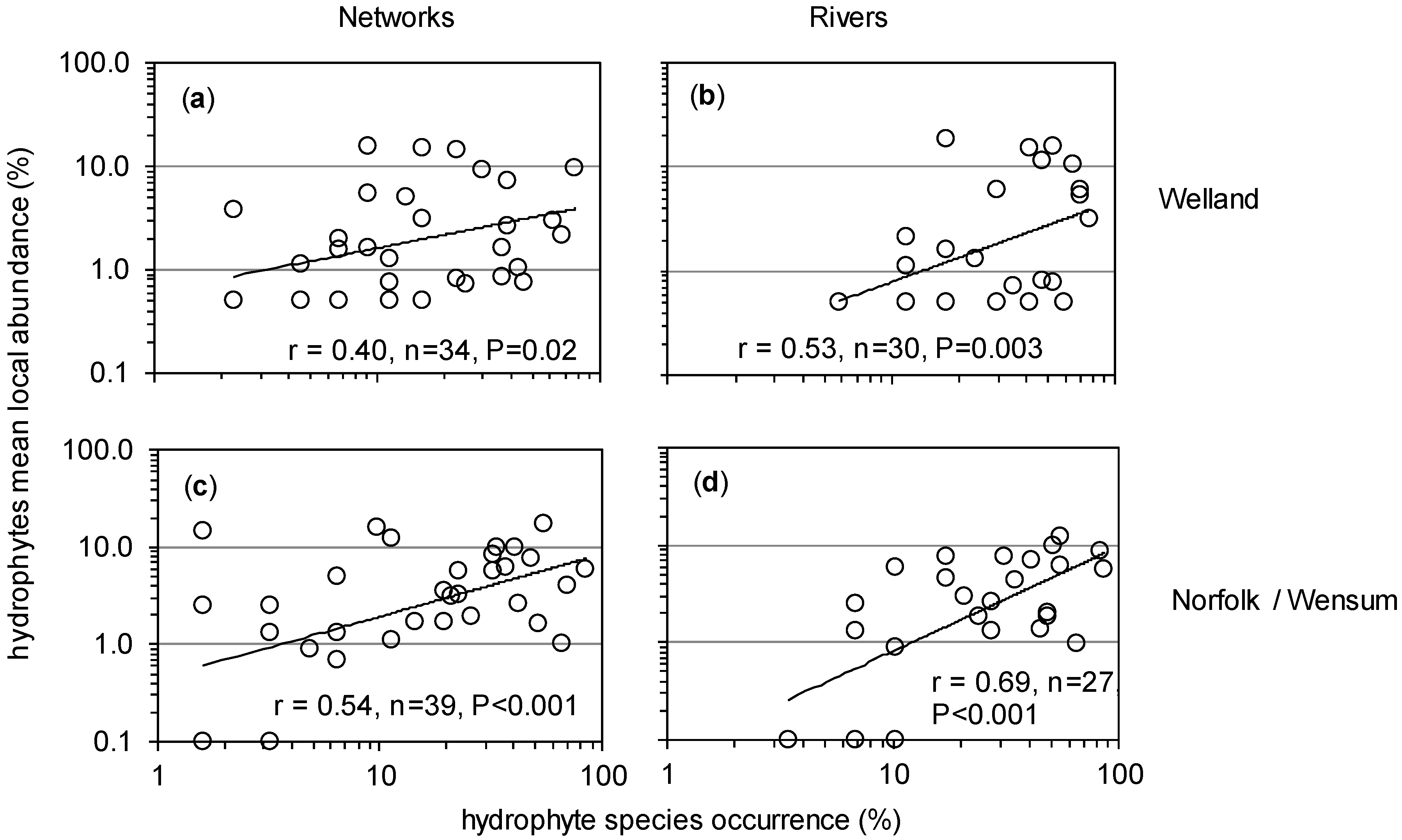
Related to that, the regression slope of local hydrophyte abundance as a function of occurrence will be steeper along rivers than across the network [41].

2. Material and Methods

2.1. Study Areas

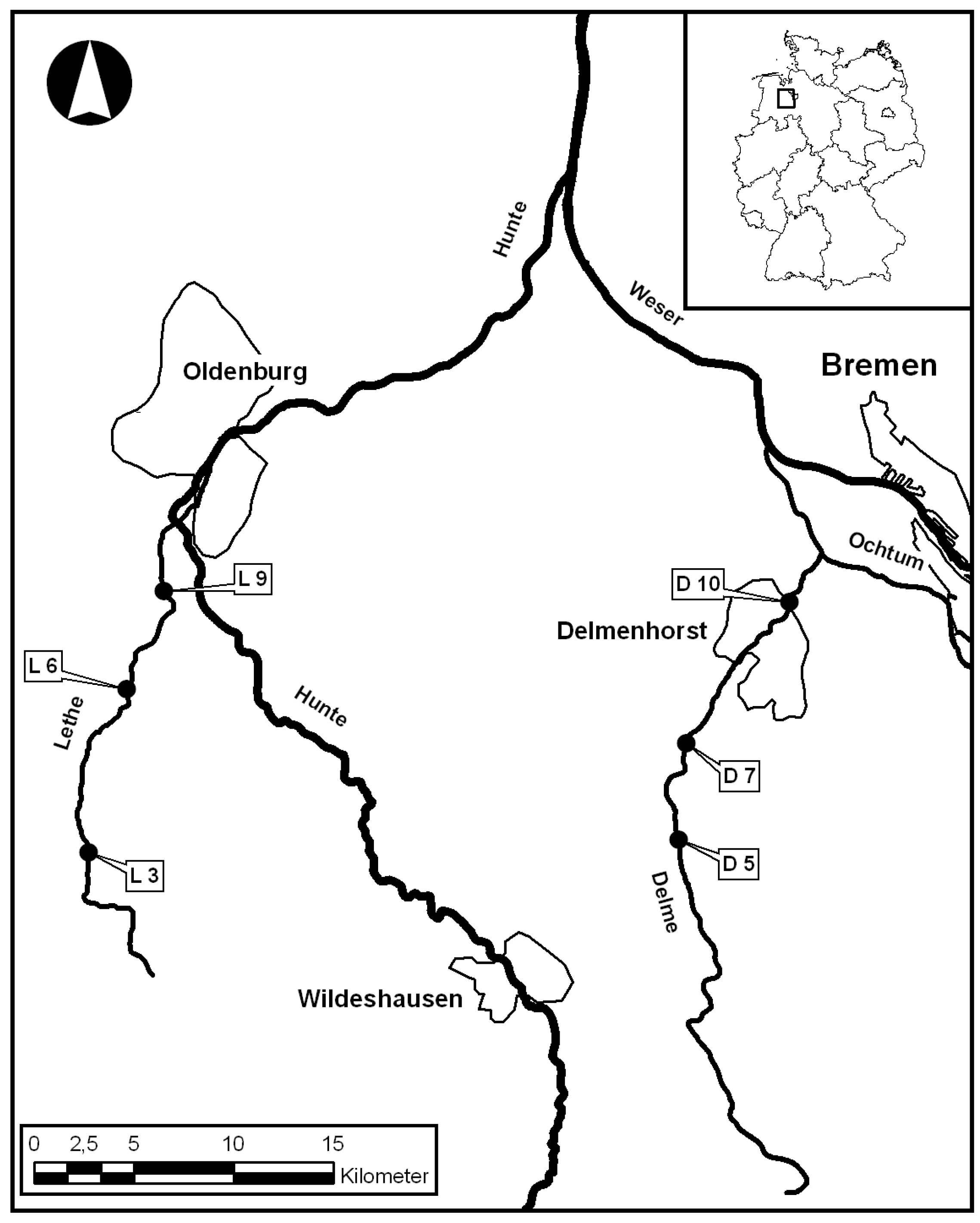
2.1.1. Rivers Lethe and Delme, Lower Saxony, Germany

The climate is under oceanic influence, with long term annual average daily temperature near freezing in January and up to 16–17 °C in the summer, and precipitation of 700 mm. The study was carried out in two lowland streams in North West Germany, River Lethe (37 km, 4th order, 180 km²) and River Delme (46 km, 3rd order, 210 km²), draining ground moraines of the Ems-Hunte moraine country (maximum elevation 89 metres OD), a natural unit formed by the penultimate (Saale) glaciation. Six reaches were selected for permanent sampling, along the upper, middle and lower sections supporting different species composition and dominance in 1978: Lethe (3, 6, 9) and Delme (5, 7, 10)—Figure 1. The substrate is mostly dominated by sand and gravel. Further information is available in Wiegleb [54,58,60,69] (in Wiegleb [54] site Lethe 6 here was called Lethe 7).

Figure 1. German river network with sampling sites.

Figure 1. German river network with sampling sites.

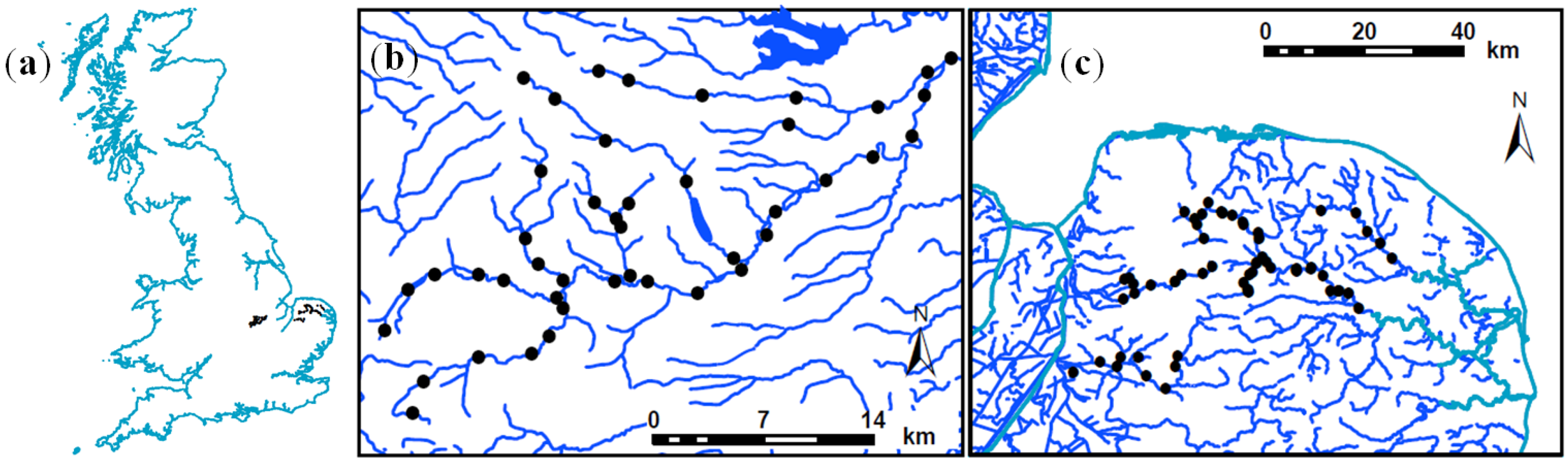
2.1.2. Norfolk Rivers, Norfolk, England

The maximum elevation (96 m OD) and climate are similar to the German sites, with long term annual average daily temperature about 4 °C in January and 17 °C in the summer, and precipitation of 670 mm. The study area is characterised by Upper Chalk solid geology overlain by quaternary deposits (chalk boulder clay; glacial sands and gravel). Four rural river basins were investigated (Figure 2): Wensum (570 km²), Wissey (275 km²), Nar (153 km²) and Bure (313 km²). River channel engineering works and weirs for water mills [71] have removed the covariation between channel cross-section area (m²) and discharge (m³ s⁻¹), and this has allowed the separation of the impact of longitudinal connectance from local physical environmental conditions (deep, slow flowing silty stretches to shallow fast flowing reaches with gravel bed; [43]. The range of average width and depth were 0.8–20.9 m and 0.1–2.0 m, respectively. For further information see [43,57].

2.1.3. River Welland Network, East Midlands, England

The river Welland basin has a similar climate to Norfolk rivers with annual rainfall of 640 mm, but the underlying geology (Lias clays with outcrop of Lincolnshire limestone) is more impervious. The upper part of the catchment has slightly more rolling hills (maximum elevation 228 m). The range of average width and depth was similar to the Norfolk rivers. The whole river network was surveyed in 1996 down to Stamford (about 500 km²)—see Figure 2 and [61,72].

Figure 2. Great Britain (a); River Welland (b) and Norfolk rivers (c) with coast and estuaries (light blue), river networks (dark blue) and sampling sites (black symbols). Maps derived from Pope [73] and Ordnance Survey OpenData™ [74]. ^©Crown copyright and database right 2013. All rights reserved. The James Hutton Institute, Ordnance Survey Licence Number 100019294.

Figure 2. Great Britain (a); River Welland (b) and Norfolk rivers (c) with coast and estuaries (light blue), river networks (dark blue) and sampling sites (black symbols). Maps derived from Pope [73] and Ordnance Survey OpenData™ [74]. ^©Crown copyright and database right 2013. All rights reserved. The James Hutton Institute, Ordnance Survey Licence Number 100019294.

2.2. Field Surveys

The survey methods used were entirely comparable because Demars and Harper [43,61] implemented the recommendations and survey method of Wiegleb [54,58,60] into the approach developed by Holmes [75]. In the Welland, field surveys were 100–500 m long (not just 500 m as stated in Demars and Harper [61]) and tended to be longer in the head waters with sampling areas mostly within 200–800 m² throughout. In Norfolk, field surveys were generally shorter (around 50 m) with longer reaches (up to 250 m) in headwaters, with similar sampling areas to the Welland (≈500 m²).

All macrophytes (mostly vascular plants) growing in the water or rooting below the water surface were recorded along relatively short river stretches by Wiegleb and colleagues; (50–70 m) and about 500 m² by Demars and colleagues, along homogeneous reaches. Demars used the species list established by Holmes [76] and also recorded a few additional taxa. The length of stream (or area) surveyed allowed recording of 66% and 76% of the species richness in all species and hydrophyte species respectively encountered over 1 km long reach [54]. The German reaches were sampled by hand or with a telescopic rake while walking along the reach on both sides and wading in the stream, wherever necessary. Wading and snorkeling was used to survey the English sites. Cover was estimated in percentages by Wiegleb and colleagues. Demars used the Braun-Blanquet [77] scale (+ present, 1 <5%, 2 5%–25%, 3 25%–50%, 4 50%–75%, 5 >75%) and Holmes [76] nine point scale (1 <0.1%, 2 0.1%–1%, 3 1%–2.5%, 4 2.5%–5%, 5 5%–10%, 6 10%–25%, 7 25%–50%, 8 50%–75%, 9 >75%). Plant specimens from Lower Saxony and Norfolk were deposited in Herbaria (LMO, LTR) and lists of taxa are provided in Appendix 1,

Table A1. List of hydrophyte and helophyte species from the rivers Lethe and Delme (Germany). The nomenclature of the vascular plants follows Stace (1997) New Flora of the British Isles 2nd Ed. Cambridge University Press [138].

Hydrophytes	Helophytes	Helophytes
Batrachospermum gelatinosum	Achillea ptarmica	Hydrocotyle vulgaris
Callitriche hamulata	Agrostis canina	Juncus articulatus
Callitriche obtusangula	Agrostis capillaris	Juncus bufonius
Callitriche platycarpa	Agrostis stolonifera	Juncus effusus
Elodea canadensis	Alisma plantago-aquatica	Lolium perenne
Elodea nuttallii	Alopecurus geniculatus	Lotus pedunculatus
Fontinalis antipyretica	Alopecurus pratensis	Lycopus europaeus
Hydrocharis morsus-ranae	Bidens cernua	Lysimachia nummularia
Lemna gibba	Bidens tripartita	Lysimachia vulgaris
Lemna minor	Botrydium granulatum	Lythrum salicaria
Leptodictyum riparium	Calamagrostis canescens	Mentha arvensis
Myriophyllum alterniflorum	Caltha palustris	Myosotis scorpioides
Nitella flexilis	Cardamine amara	Rorippa nasturtium-aquaticum
Nuphar lutea	Carex acuta	Persicaria hydropiper
Oenanthe aquatica	Carex paniculata	Phalaris arundinacea
Persicaria amphibia	Deschampsia cespitosa	Poa palustris
Potamogeton alpinus	Eleocharis acicularis	Poa trivialis
Potamogeton berchtoldii	Eleocharis palustris	Ranunculus repens
Potamogeton crispus	Epilobium hirsutum	Rorippa amphibia
Potamogeton natans	Epilobium obscurum	Rorippa palustris
Potamogeton perfoliatus	Epilobium palustre	Rorippa sylvestris
Potamogeton trichoides	Epilobium roseum	Rumex acetosa
Ranunculus peltatus	Equisetum palustre	Rumex hydrolapathum
Sagittaria sagittifolia	Galium palustre	Rumex obtusifolius
Sparganium emersum	Galium uliginosum	Scirpus sylvaticus
Sparganium erectum	Glechoma hederacea	Solanum dulcamara
Spirodela polyrhiza	Glyceria fluitans	Stachys palustris
	Glyceria maxima	Stellaria uliginosa
	Holcus mollis	Veronica beccabunga

,

Tabel A2. List of hydrophyte and helophyte species from the River Welland (England). The nomenclature of the vascular plants follows Stace (1997) New Flora of the British Isles 2nd Ed. Cambridge University Press [138].

Hydrophytes	Helophytes
Alisma plantago-aquatica	Angelica sylvestris
Amblystegium riparium	Carex acuta
Apium nodiflorum	Carex acutiformis
Butomus umbellatus	Cirsium palustre
Callitriche spp.	Epilobium hirsutum
Elodea canadensis	Equisetum fluitans
Elodea nuttallii	Equisetum palustre
Fontinalis antipyretica	Glyceria maxima
Glyceria fluitans	Iris pseudacorus
Lemna gibba	Juncus effusus
Lemna minuta/minor	Juncus inflexus
Mentha aquatica	Persicaria maculosa
Myosotis scorpioides	Petasites hybridus
Myriophyllum spicatum	Phalaris arundinacea
Nuphar lutea	Ranunculus repens
Nymphoides peltata	Rorippa amphibia
Oenanthe fluviatilis	Rumex sp.
Persicaria amphibia	Scirpus sylvaticus
Potamogeton crispus	Scrophularia auriculata
Potamogeton natans	Solanum dulcamara
Potamogeton obtusifolius	Typha latifolia
Potamogeton pectinatus	Urtica dioica
Potamogeton perfoliatus	Veronica catenata
Potamogeton x salicifolius
Ranunculus subgenus Batrachium
Rhynchostegium riparioides
Rorippa-nasturtium aquaticum
Sagittaria sagittifolia
Schoenoplectus lacustris
Sparganium emersum
Sparganium erectum
Veronica anagallis-aquatica
Veronica beccabunga
Zannichellia palustris

and

Table A3. List of hydrophyte and helophytes species from Norfolk rivers (England). The nomenclature of the vascular plants follows Stace (1997) New Flora of the British Isles 2nd Ed. Cambridge University Press [138].

Hydrophytes	Helophytes
Amblystegium riparium	Agrostis stolonifera
Berula erecta	Apium nodiflorum
Butomus umbellatus	Caltha palustris
Callitriche obtusangula/platycarpa	Carex sp.
Ceratophyllum demersum	Epilobium hirsutum
Chara globularis	Equisetum fluviatile
Elodea canadensis	Equisetum palustris
Elodea nuttallii	Eupatorium cannabinum
Fontinalis antipyretica	Glyceria maxima
Glyceria declinata/notata/fluitans	Iris pseudacorus
Groenlandia densa	Juncus inflexus
Hippuris vulgaris	Juncus subnodulosus
Hottonia palustris	Lycopus europaeus
Lemna minor/minuta	Mentha aquatica
Lemna trisulca	Mimulus guttatus
Myriophyllum spicatum	Myosites scorpioides
Myriophyllum verticillatum	Phalaris arundinacea
Nitella flexilis	Phragmites australis
Nuphar lutea	Ranunculus repens
Nymphaea alba	Rorippa nasturtium-aquaticum
Oenanthe fluviatilis	Rumex sp.
Pellia sp.	Scrophularia auriculata
Potamogeton alpinus	Solanum dulcamara
Potamogeton crispus	Typha latifolia
Potamogeton friesii	Veronica beccabunga/catenata
Potamogeton lucens
Potamogeton pectinatus
Potamogeton perfoliatus
Potamogeton pusillus
Ranunculus penicillatus/trichophyllous
Ranunculus circinatus
Ranunculus fluitans
Riccia natans
Sagittaria sagittifolia
Schoenoplectus lacustris
Sparganium emersum
Sparganium erectum
Veronica anagallis-aquatica
Zannichellia palustris

.

The German data were collected monthly for 25 consecutive months from March 1979 to March 1981 and yearly (June to September) for 21 consecutive years (1978–1998). Summer vegetation (June to September) was recorded during one (1978, 1994, 1996–1998), two (1981–1993, 1995) or four (1979–1980) visits per year at each site. The highest species cover value observed among several surveys within one summer was selected. We checked for bias in species richness due to those differences in sampling effort (one to four surveys). The years with one survey were all in June or July. We used the years with two surveys (1981–1993), one in June/July and one in August/September to check for bias in sampling effort. Significantly higher species richness and total cover (sum of individual species cover) were found when two surveys were conducted (Table 1). Only five years had one survey, so we decided to correct the sampling bias by adding the observed difference. Richness and total cover of hydrophyte species were corrected according to the results of Table 1 for the years 1978, 1994, 1996–1998. These corrections were generally small and affected years at both ends of the time series. There were no significant differences in summer species richness and cover when quantified from two (June/July and August/September) or four (monthly) surveys.

Table 1. Differences in species richness, total cover (%) and attribute group richness (±sem) between two and one summer surveys (period 1981–1993) at the six sites surveyed in the rivers Lethe and Delme.

Differences in	L3	L6	L9	D5	D7	D10
Species richness	0.8 ± 0.3	1.0 ± 0.2	0.8 ± 0.2	2.6 ± 0.4	3.4 ± 0.5	1.5 ± 0.5
Total cover	20 ± 4	28 ± 6	27 ± 4	40 ± 5	33 ± 4	16 ± 5
Attribute group richness	0.4 ± 0.2	0.5 ± 0.2	0.6 ± 0.2	2.0 ± 0.4	1.9 ± 0.4	1.4 ± 0.4

Table 1. Differences in species richness, total cover (%) and attribute group richness (±sem) between two and one summer surveys (period 1981–1993) at the six sites surveyed in the rivers Lethe and Delme.

Differences in	L3	L6	L9	D5	D7	D10
Species richness	0.8 ± 0.3	1.0 ± 0.2	0.8 ± 0.2	2.6 ± 0.4	3.4 ± 0.5	1.5 ± 0.5
Total cover	20 ± 4	28 ± 6	27 ± 4	40 ± 5	33 ± 4	16 ± 5
Attribute group richness	0.4 ± 0.2	0.5 ± 0.2	0.6 ± 0.2	2.0 ± 0.4	1.9 ± 0.4	1.4 ± 0.4

In England, 44 sites of the River Welland were surveyed in summer 1996 (June–July), and 62 sites in Norfolk were surveyed in summer 1999 and 2000. Twelve sites along the River Wensum were sampled annually during summer 1999, 2000 and 2001.

2.3. Community Structure Indices

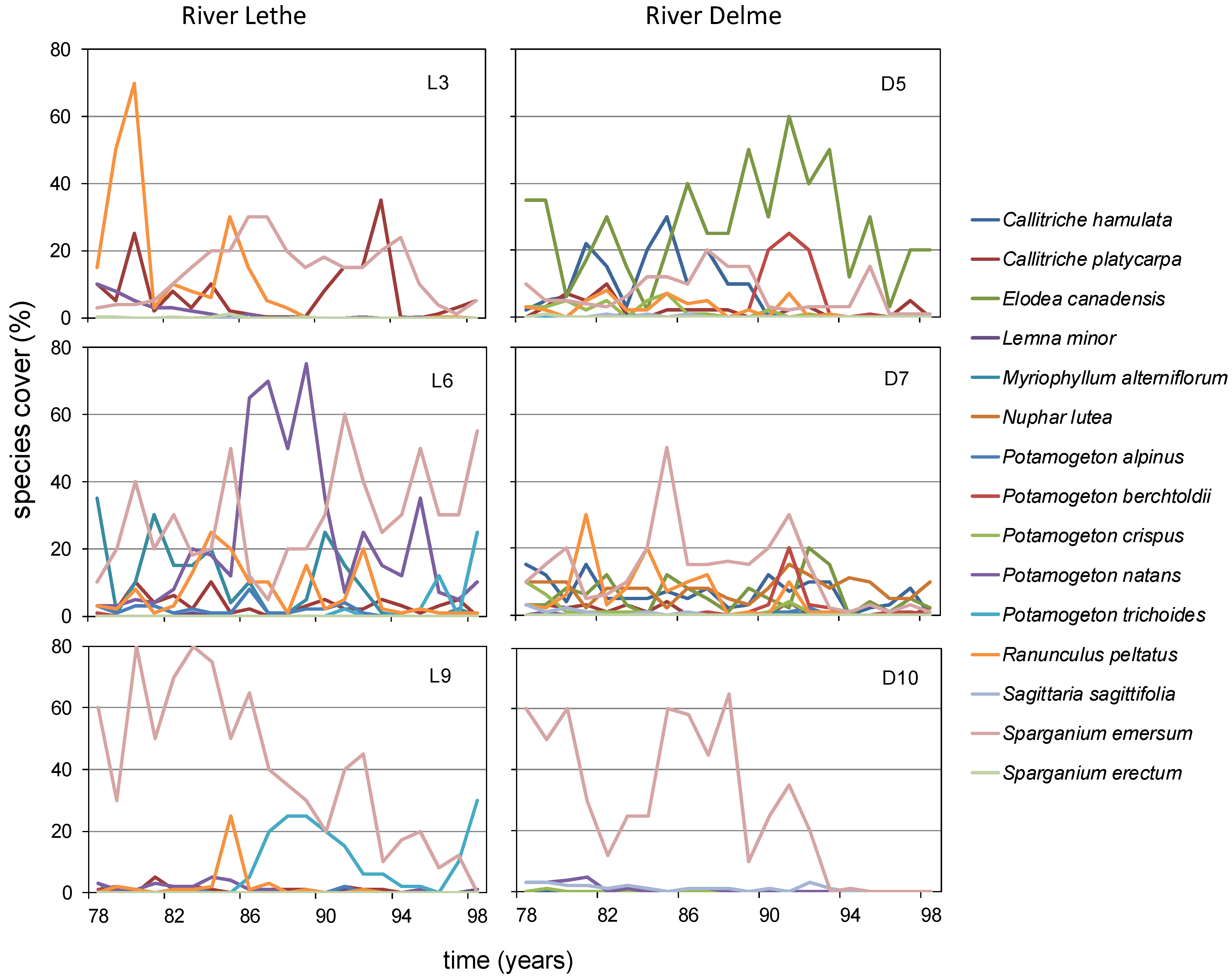
2.3.1. Individual Species Cover

Percentage abundance data were used for all community structure indices. This meant transforming the Braun-Blanquet scale back to percentages as follows: + 0.1%, 1 2.5%, 2 15%, 3 37.5%, 4 62.5%, 5 87.5%, and similarly for the Holmes 1999 scale (1 0.05%, 2 0.5%, 3 1.75%, 4 3.75%, 5 7.5%, 6 17.5%, 7 37.5%, 8 62.5%, 9 87.5%). Most analyses were also run on presence absence data to see how abundance affected the results. Filamentous green algae were considered as biotic competitor and entered as exogenous factor (see below).

A distinction was made between hydrophytes (species mostly present in the channel) and helophytes (marginal species mostly established along the river bank) following Wiegleb [54], Willby et al. [68] and Demars and Harper [43] in order to investigate the edge effect (see introduction)— Appendix 1, Table A1, Table A2 and Table A3.

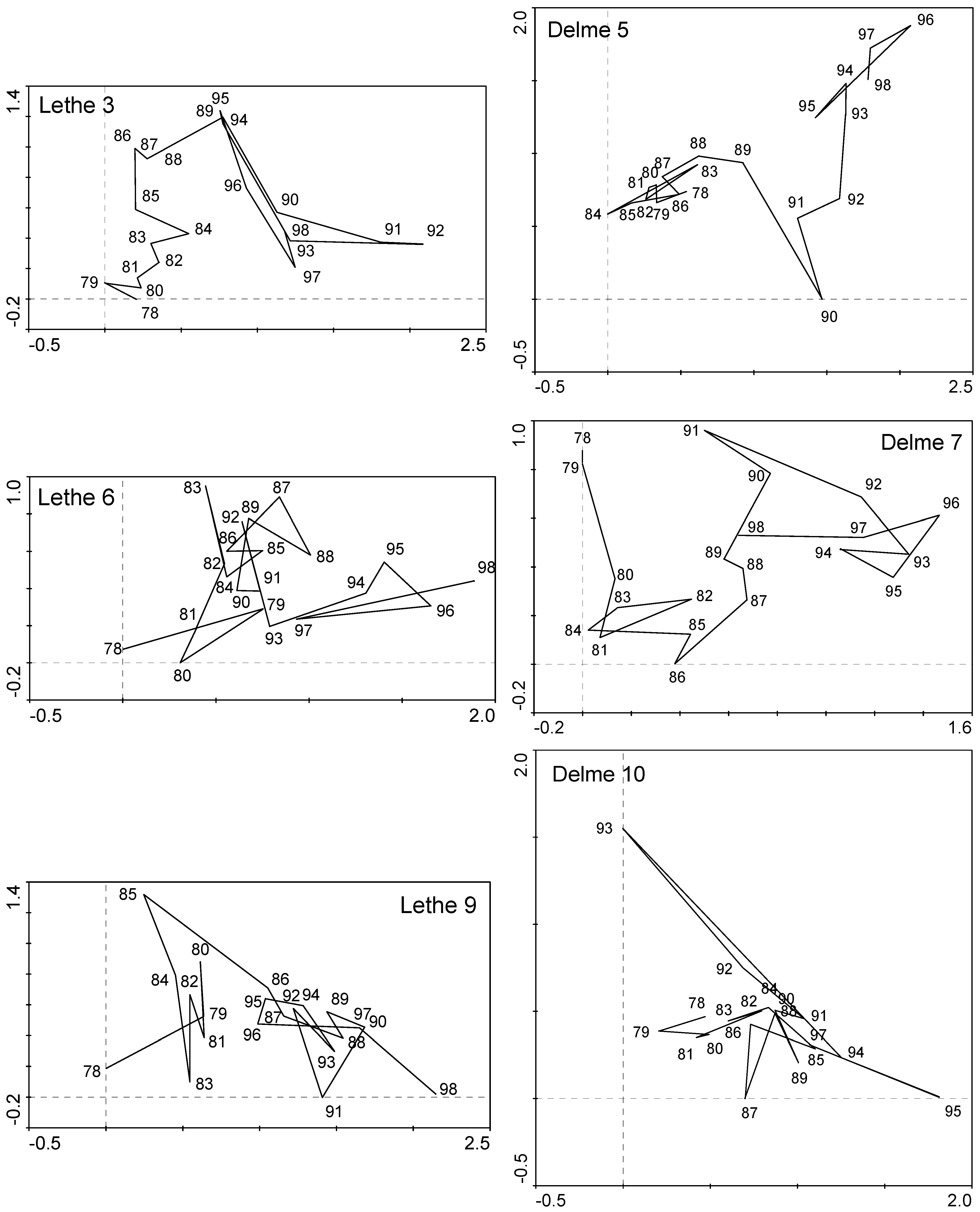
2.3.2. Unconstrained Ordinations

Change in species composition over time was investigated with Detrended Correspondence Analysis (DCA) using log(x + 1) transformed species abundance data. Species present in less than three surveys across all sites were not selected. The rare species within sites were down weighted for the DCA of individual sites. CA were detrended by segments using Canoco 4.5 to obtain estimates of gradient lengths in standard deviation units of species turnover [78]. These analyses were essential to interpret the multivariate autocorrelations.

2.3.3. Autocorrelation

Change in species composition between pairs of sites within time step or distance classes were investigated with multivariate Mantel tests. Species abundance was log(x + 1) transformed prior to analyses, similarly to the DCA. Site (or year) similarity matrices based on Euclidean distance of species abundance data (or Jaccard index for species presence absence data) of the site (or year) × species matrices were computed for every pairs of sites using Genstat 16 [79]. Time intervals and geographical distances between dates and sites were also calculated and Excel was then used to produce similarity matrices for the various time intervals and distance classes as in Legendre and Legendre ([80], p. 737). All similarity matrices were then standardized to zero mean and unit variance. The cross product of the unfolded matrices was calculated with Genstat and multiplied by 1/(1/d), where d = [n(n−1)/2] is the number of distances in the upper triangular part of each matrix ([80], p. 554), in order to calculate the standardized Mantel statistic (range −1 to 1). The Mantel test was computed in Genstat. Significant tests were indicated by a filled symbol on the autocorrelograms. Two types of corrections for multiple testing were applied. For the monthly time series a Bonferroni correction of α = 0.05/k, with k number of time classes was applied since we expected positive autocorrelations in the lowest and highest classes. For the yearly time series and all spatial analyses a progressive Bonferroni correction of α = 0.05/k for the kth time or distance class was applied as we expected positive autocorrelations in the first few classes only ([80], p. 738). Positive Mantel statistics represented positive autocorrelation.

In order to infer the potential role of dispersal (endogenous factor) to explain positive spatial autocorrelation, it was necessary to also look for potential spatial autocorrelations in exogenous factors (here depth, substrate). Spatial autocorrelation analysis was also performed on a site similarity matrix based on pDCA axes (partial detrended correspondence analysis) of the species × site matrix where the effect of exogenous factors (depth, substrate) on species composition had been removed.

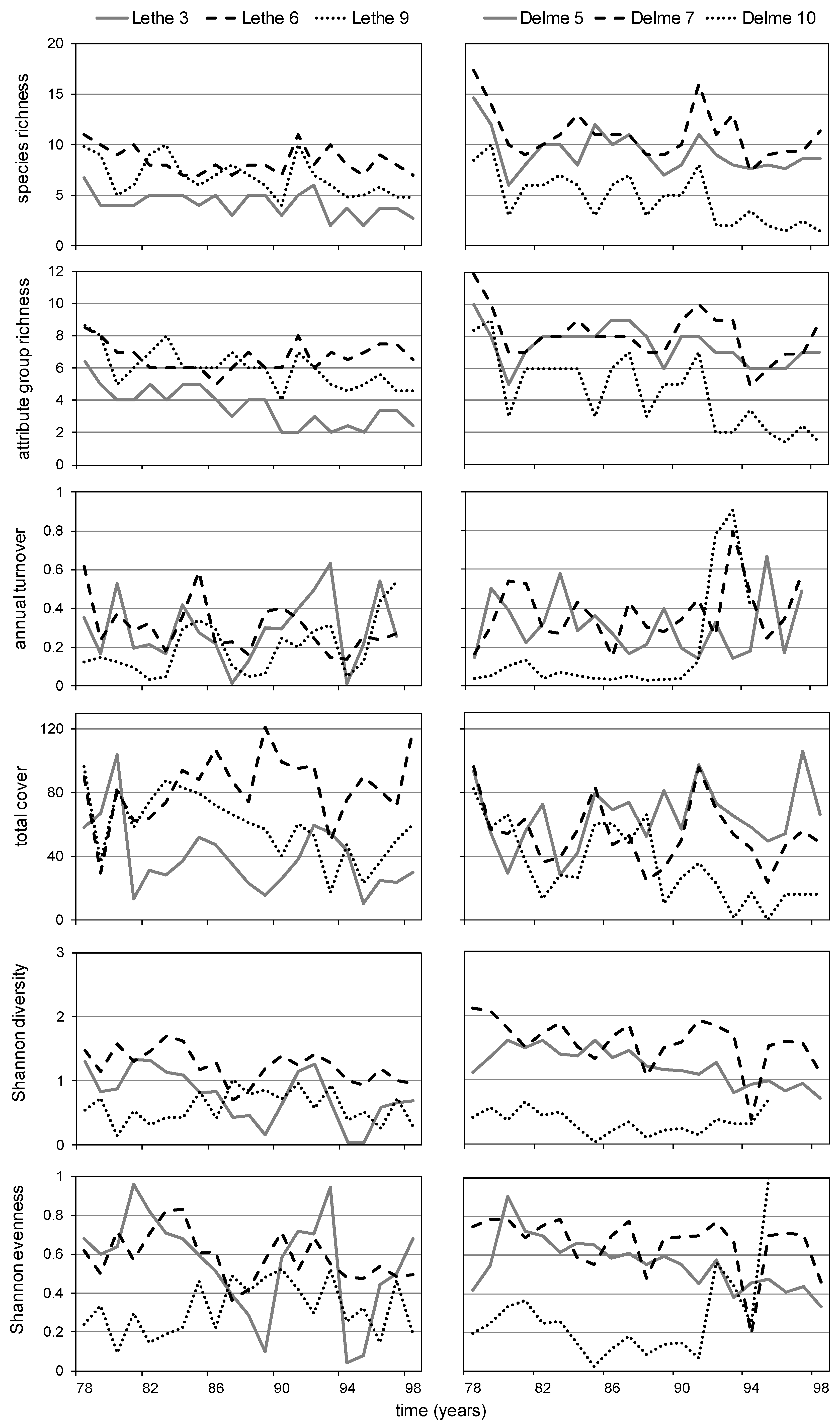
2.3.4. Richness, Total Cover and Turnover

Richness was the total number of species (S) observed at a site at a given time. Total cover was calculated by adding the percentage cover of individual species. The temporal (inter-annual) and spatial (inter-site) species turnover Sτ was calculated as in Tokeshi [81]:

(1)

where P_i(t) and P_i (t + 1) are the proportional abundance of species i in sample t and t + 1 respectively; and n is the total number of species occurring on the two occasions (or sites).

2.3.5. Shannon Diversity (H') and Evenness (J')

The indices were computed as follows:

(2)

(3)

with S total number of species; and P_i proportional abundance of species i in sample (here site or year). Note that H' is resulting from both species richness and evenness, and J' ranges from 0 to 1. The more similar abundances among species are, the higher is J'.

2.3.6. Species Range-Abundance Patterns

The log of species mean local abundance was plotted against the log of species frequency of occurrence (range) as in Riis and Sand-Jensen [41]. The spatial datasets were divided into the main rivers (Wensum, Welland) and the whole networks.

2.4. Environmental Variables

2.4.1. Rivers Lethe and Delme

The geographical, physical (e.g., depth, substrate) and chemical (including nitrate, phosphate) aspects remained largely unchanged over the whole period (1978–1998) and are not considered further in this study focusing on temporal changes (see [60]). Shading, however, did change over time at some sites and was estimated from field observations. Filamentous algae were considered competitors to the vascular plant flora and were included in the analysis as an exogenous biotic factor (0 absent, 1 <1%, 2 1%–10%, 3 >10% cover). These rural rivers are also highly managed and suffer from various pressures such as weed cutting. This is rather typical of European lowland rivers with potential impacts on aquatic plant composition and diversity [82,83]. Weed cutting events were recorded and binary coded 0/1 for absence/presence.

Average mean daily discharge was available from the Lower Saxon State Department for Waterway, Coastal and Nature Conservation. The timing, magnitude and frequency of hydrological extremes have been shown to affect river plants [34,84]. In order to keep the number of environmental variables to a minimum, four variables were considered: number of days with discharge below Q₉₅ (5% lowest flows) during the vegetation period (June–September) and exceeding Q₁₀ (10% highest flows) prior, during and after the growing season (October–January, Feburary–May, June–September).

Local weather data were taken from the meteorological station of Bremen airport for which mean daily temperature and sunshine duration measurements were provided by the Federal Ministry of Transport, Building and Urban Development. Two variables were derived: number of winter and summer days with temperature less than −10 °C (leading to ice formation in rivers) and above 20 °C, respectively.

Regional changes in weather were also investigated with the North Atlantic Oscillation (NAO) index, taken from National Oceanic and Atmospheric Administration (NOAA) [85]. They were differentiated according to winter (December, January, February), summer (June, July, August) and the whole year.

2.4.2. River Welland and Norfolk Rivers

Aquatic plant composition changed mostly according to substrate (silt, gravel), depth and spatial connectivity [43,61]. Further analyses were undertaken here to test the effects of the same exogenous factors on community structure indices using regression analyses (richness, total cover, turnover, diversity and evenness).

2.5. Linking Vegetation with Time and Environmental Data

The aim was to test whether the vegetation changed over time in the rivers Lethe and Delme and whether this could be related to more specific drivers. We focused on hydrophyte species with at least three records (23 species) because of the sampling artifact regarding marginal plants (edge effect). The data were centered and standardized prior to analysis. Partial stepwise multiple regression analyses were used to test whether total cover, species richness, attribute group richness, species turnover, diversity, and evenness were related to time and environmental data. We used all sampling occasions at the six sites (total of 6 × 21 = 126) in these analyses but removed the effect of sites (spatial differences) before running 9999 Monte Carlo random cyclic shift permutation tests in order to keep the temporal structure of the data (due to temporal autocorrelation, see ter Braak and Šmilauer ([78], p. 45)). The inter-annual species turnover was related to time and environmental variables for the period 1979–1998 (there being 20 values for the 21 years). We used partial stepwise canonical correspondence analyses (pCCA) for the species composition data using log(x + 1) transformed abundance data. All analyses were run with Canoco 4.5 [78]. Since we had many environmental variables (13) we applied a Bonferroni correction for the statistical level of significance with α = 0.05/13 = 0.004. We searched for the most parsimonious model, alternating order of inclusion of explanatory variables with similar size effects.

We used the species traits (attributes) of Willby et al. [68] to investigate changes of endogenous factors over time and against the environmental variables using the same statistical design. In order to solve the 4th corner problem [86], the “attribute × sites” matrix was generated with the matrix product of “attribute × species” times “species × sites” using Genstat. The “attribute × site” matrix could then be related to the “environmental variables × site” using redundancy analysis (RDA) which was more appropriate for the species attribute (traits) composition [68]. We used all sampling occasions at the six sites (total of 6 × 21 = 126) and the same statistical tests as above for the species composition analyses, using partial RDAs. The RDA also produced a summary table of all individual correlations between attributes and selected environmental variables. This is a slightly different approach to Demars and Harper [43] which had first synthesized the species trait information into natural combination of attributes. The main criticism is that traits and their modalities (or attributes) are not phylogenetically independent and so some correlations between traits and environmental factors may reflect the contingency of evolution rather than adaptation [87]. Expected mechanisms and trade-off in species traits (e.g., regeneration and dispersal traits with spatial connectivity; growth form with depth, substrate) will guide interpretation (see [31,43,65,68]). The attribute groups of hydrophytes defined by Willby et al. [68] represented natural combination of attributes and were used here to quantify the change in species trait diversity.

2.6. Statistical Analyses for Spatial Patterns

For the spatial analyses, linear, split line or second order polynomial regression equations were used according to previous findings for riparian and aquatic species richness along rivers [38,59,61,88,89,90]. The probabilities were derived from 999 random Monte Carlo permutations restricted for spatial structure (random cyclic shift) after ranking the sites by distance from source, a more simple and pragmatic approach than Peterson and Hoef [91]. Richness was also standardised for small differences in area (for hydrophytes) or length (for helophytes) of survey as in previous studies [89]: S_standardised = S/log₁₀ (area or length). Regression analyses were performed with Genstat 16 and Canoco 4.5.

In order to calculate the species diversity across the river network, species richness was quantified from sites belonging to different distance classes with about 9 (±1 se) sites per class.

In order to compare hydrophyte local abundance-occurrence patterns, we tested for differences in the correlation coefficient using the z test (two tailed p value, [92]) and differences in the rate of increase of species abundance against occurrence (slope) using the Student’s t test computed as the difference between the two slopes divided by the standard error of the difference between the slopes (two tailed p value, with N-4 degree of freedom, [92]). These tests were performed across the two river networks (Welland with 44 sites and Norfolk with 62 sites), as well as along rivers using the River Welland (17 sites) and River Wensum (29 sites).

Spatial autocorrelations were computed along the main rivers (Wensum, Welland, Canada) and across whole networks. Distance from source and the distance between sites along rivers were based on measured river length with an opisometer from 1/50000 Ordnance Survey maps. The distance between sites across the whole network was simply computed as straight lines using Geospatial Modelling Environment (GME 0.7.2.1 RC2 for ArcGIS 10.1 and R2.12+, [93]). Similarly to the temporal study total cover, attribute group richness, species turnover (Sτ), species diversity (H'), species evenness (J'), were also related to distance from source and the probabilities derived as above. Only sites with more than two species and five percent cover were used for Sτ, H', and J'.

3. Results

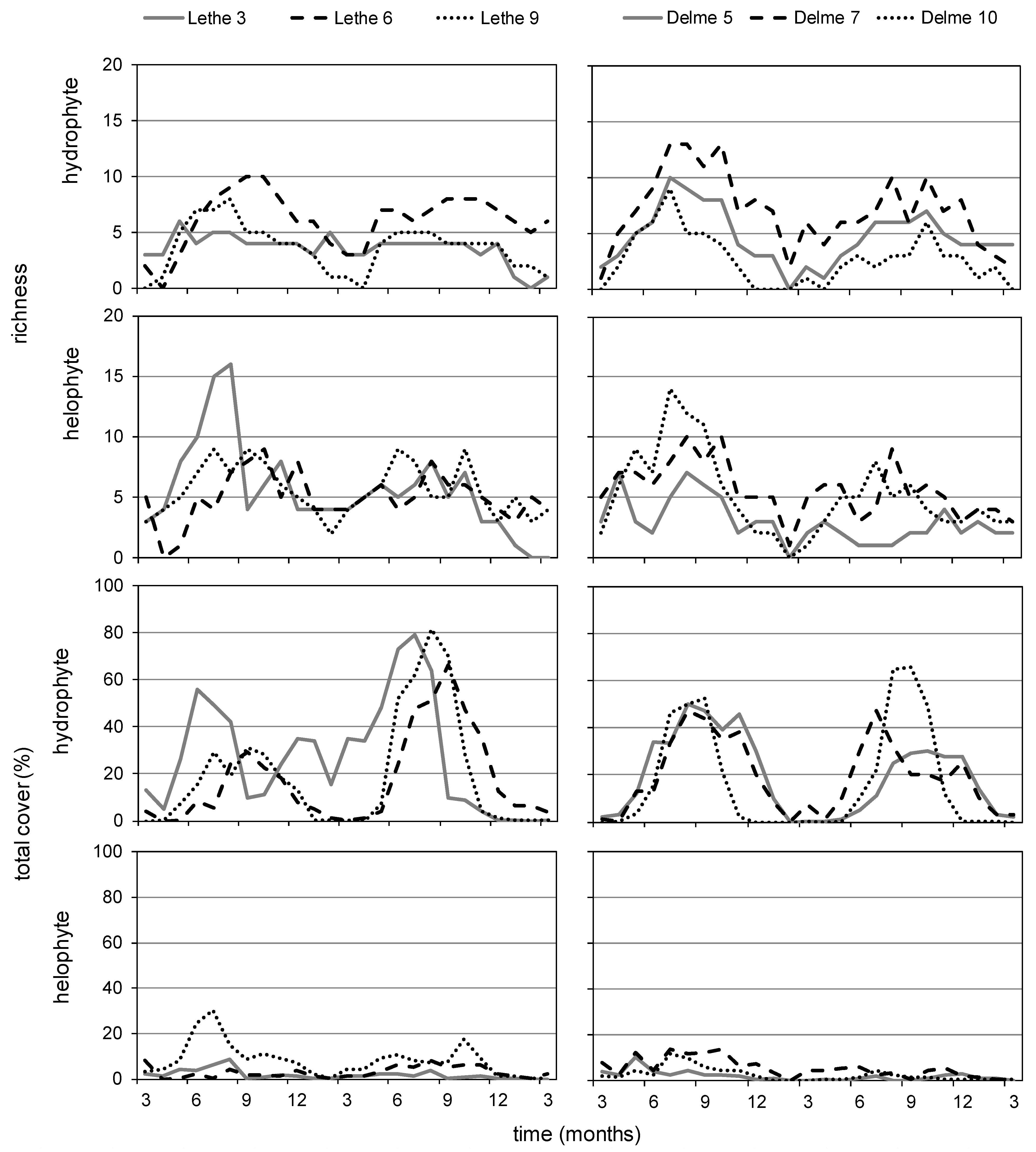
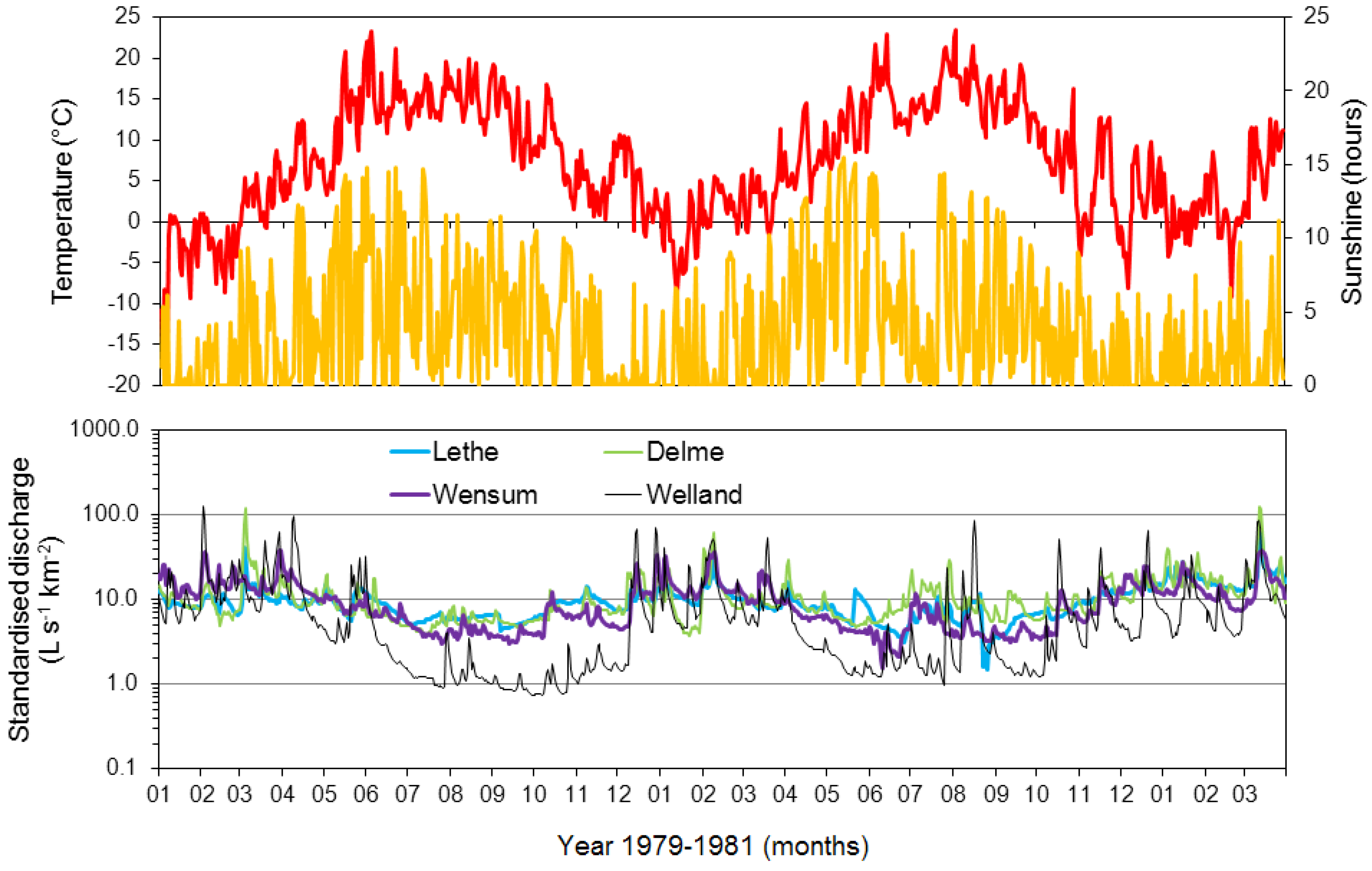
3.1. Lethe-Delme Monthly Changes over Two Years

Both hydrophyte species richness and cover generally reached a maximum during summer and autumn and a minimum in late winter, with some asynchrony in the patterns (Figure 3). This corresponded to the daily change in sunshine duration, mean daily air temperature and discharge (Appendix 2, Figure A1). Helophyte species richness was similar to hydrophyte species richness, but total cover remained generally below 10%.

The temporal autocorrelation of hydrophyte species composition was generally significantly positive at 1–2 and 12 months’ time intervals, and negative at six months’ intervals (Figure 4). Helophytes temporal autocorrelation was markedly different however, with only positive autocorrelation at 1–2 months’ time interval.

Figure 3. Monthly changes (March 1979 to March 1981) in richness and total cover (%) in hydrophyte and helophytes at six sites from the rivers Lethe and Delme (Lower Saxony, Germany).

Figure 3. Monthly changes (March 1979 to March 1981) in richness and total cover (%) in hydrophyte and helophytes at six sites from the rivers Lethe and Delme (Lower Saxony, Germany).

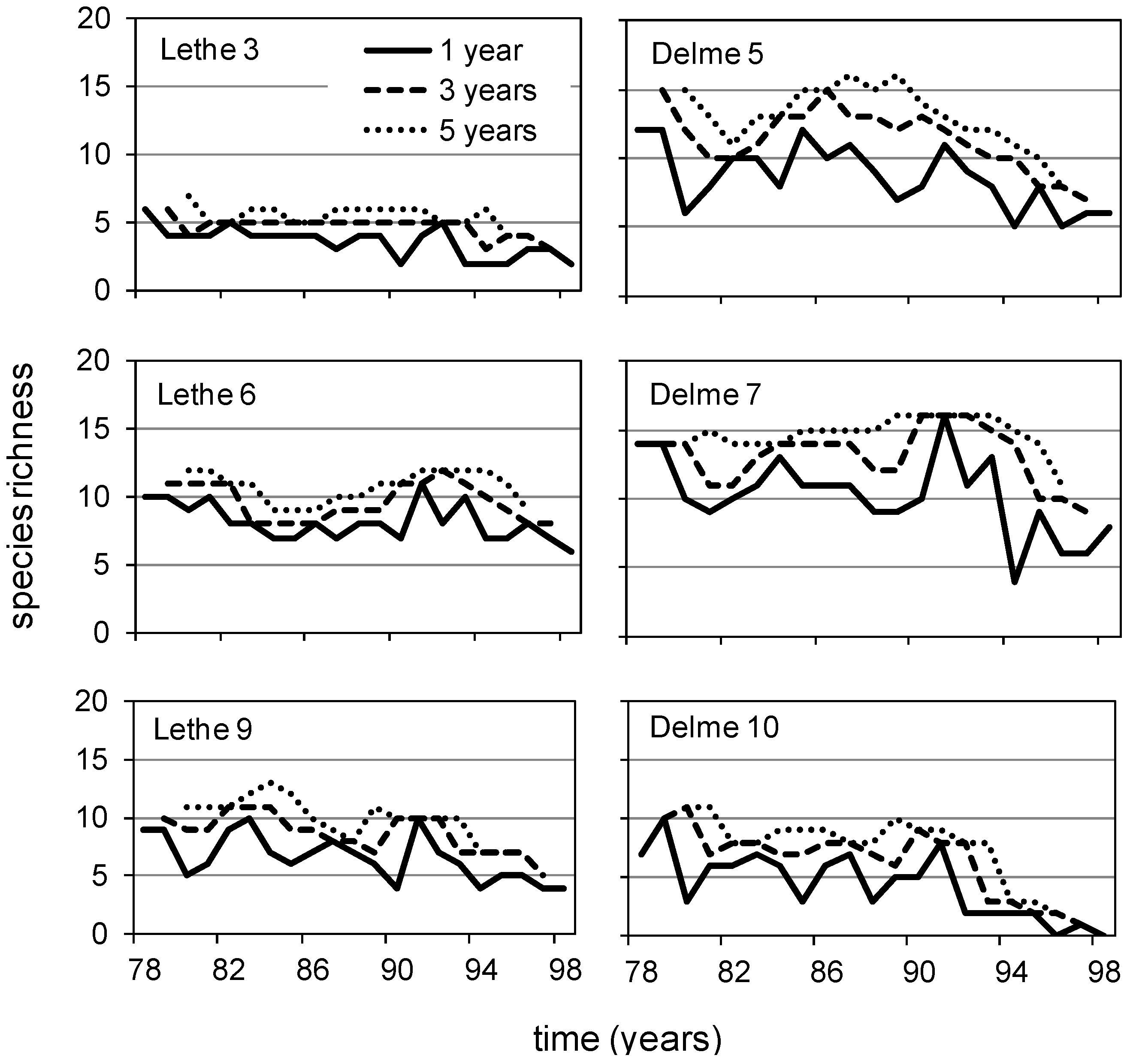
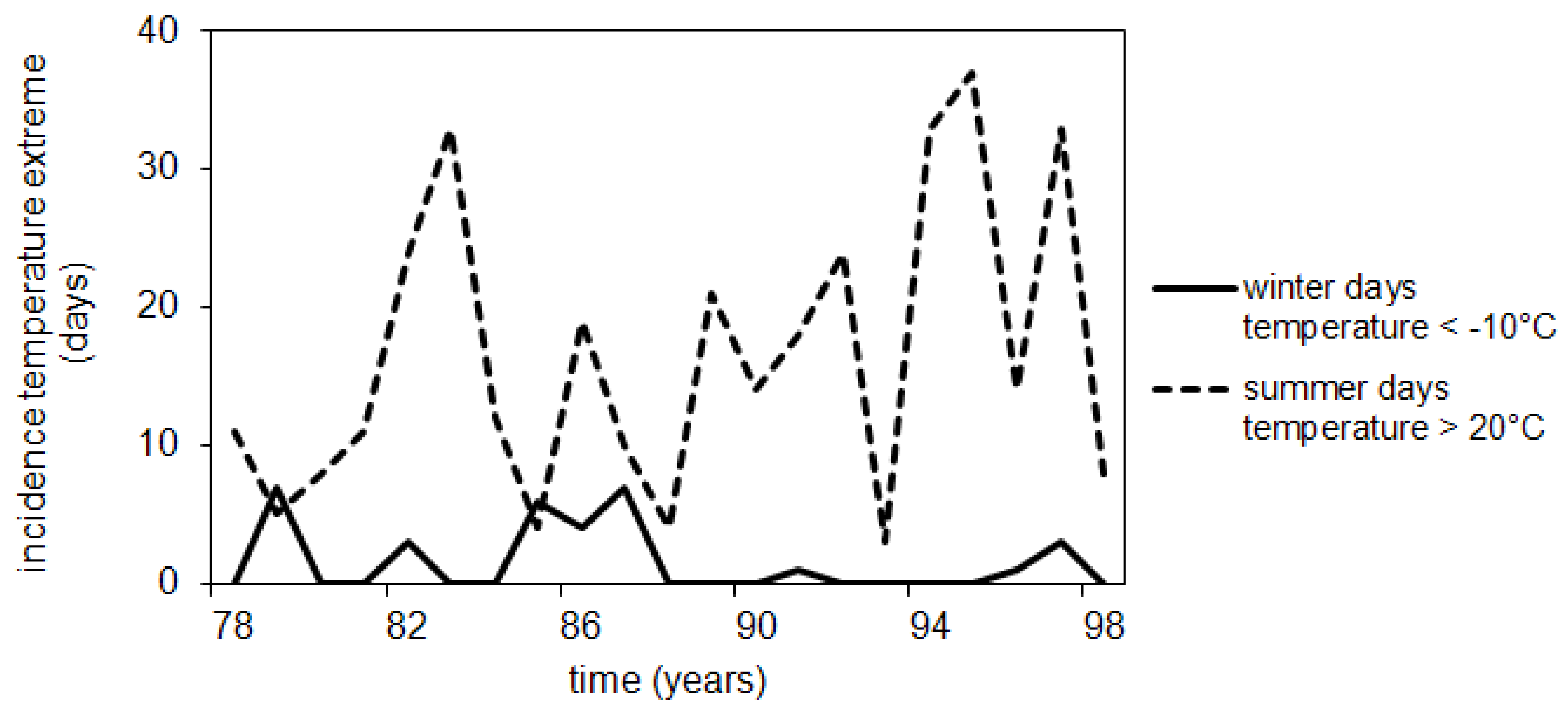
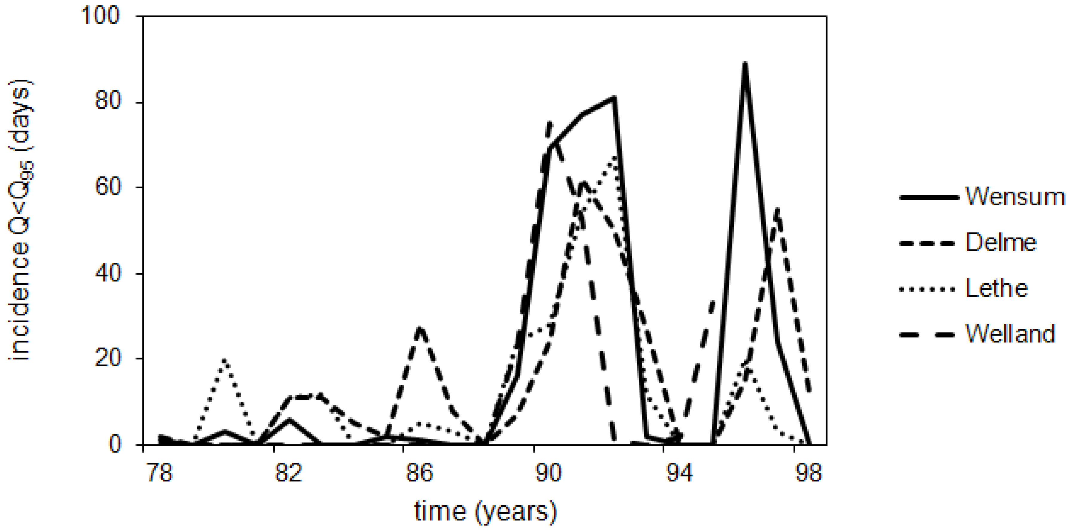
3.2. Lethe-Delme Temporal Changes over 21 Consecutive Years

The incidence of high flows prior, during and after the plant growing season (Appendix 2, Figure A2) and summer high temperatures (Appendix 2, Figure A3) were very variable between years, with no obvious trend over the 21 years record. English rivers showed similar flow patterns to the German rivers (Appendix 2, Figure A2). Climate warming during the observation period 1978–1998 was characterised by marked differences in low flows and low winter temperature (corresponding to river icing) between the first and second half of the period (Appendix 2, Figure A3 and Figure A4). This was not reflected in the yearly or seasonal NAO indices which were always positive and showed relatively little variability (mostly 0.5 < NAO < 2.5).

Figure 4. Temporal autocorrelograms of plant species composition at monthly time steps. Significant tests are indicated by a filled symbol (after Bonferroni correction of α = 0.05/k). Mantel statistics range from −1 to 1. Positive Mantel statistics represent positive autocorrelation. Number of comparisons per class ranged from 39 to 57.

Figure 4. Temporal autocorrelograms of plant species composition at monthly time steps. Significant tests are indicated by a filled symbol (after Bonferroni correction of α = 0.05/k). Mantel statistics range from −1 to 1. Positive Mantel statistics represent positive autocorrelation. Number of comparisons per class ranged from 39 to 57.

Regarding the other exogenous factors, there were more weed cutting events recorded in the first half of the period in the river Lethe, and vice versa in the Delme, with two to six weed cutting events recorded at individual sites over the 21 years. Shading stayed stable at four sites and increased substantially from 20% to 50% and 10% to 50% at L3 and L9 respectively. While L6 and D5 tended to have more green algae than the other sites, there were no obvious temporal changes.

Individual species cover was rather stochastic (Figure 5). While many sub-dominant taxa were regularly present in the upper and middle section of the rivers, they were absent from the lower sites (L9, D10). There were a lot of changes in the dominant taxa. Sparganium emersum decreased considerably at the lower sites of both rivers (L9, D10).

Hydrophytes temporal autocorrelation was generally significantly positive at short time intervals (1–3 years), but surprisingly negative at long time steps (>10 years)—Figure 6. The pattern for helophytes was markedly different with negative autocorrelation at intermediate time intervals (4–9 years) and positive at both short (1–3 years) and long time lags (>13 years). Because of these striking differences and edge effect artefact, the remaining analyses focus on hydrophytes only.

Figure 5. Temporal dynamics of the 15 most frequent hydrophyte species recorded in the rivers Lethe and Delme over 21 consecutive years.

Figure 5. Temporal dynamics of the 15 most frequent hydrophyte species recorded in the rivers Lethe and Delme over 21 consecutive years.

Changes in hydrophyte composition over 21 years span an amazing two standard deviation units of species turnover on the DCA, which is about 50% species turnover (Figure 7). Most sites show two distinct centroids with some random movement around, that is a change of state confirmed by the significant negative autocorrelations and overall (across all sites) significant effect of time explaining 9% of the variability in species composition change (pCCA, P < 0.0001).

Over time, hydrophyte richness (r² = 0.23, P < 0.0001), attribute group richness (r² = 0.27, P < 0.0001) and Shannon diversity (r² = 0.18, P = 0.001) all decreased; while turnover (r² = 0.03, P = 0.11), cover (r² = 0.05, P = 0.034) and evenness (r² = 0.04, P = 0.14) did not show a significant trend (after Bonferroni correction)—Figure 8.

Figure 6. Temporal autocorrelograms of plant species composition at yearly time steps at six sites from the rivers Lethe and Delme (Lower Saxony, Germany). Note the similarities and differences in patterns within and between hydrophytes and helophytes. Significant tests are indicated by a filled symbol (after progressive Bonferroni correction of α = 0.05/k for the kth distance class). Mantel statistics range from −1 to 1. Positive Mantel statistics represent positive autocorrelation. Number of comparisons per class ranged from 21 to 57; except for D10 (12–48 comparisons) from which the analyses were based on the first 18 years of the time series, there being no species in two of the last three years (1996, 1998).

Figure 6. Temporal autocorrelograms of plant species composition at yearly time steps at six sites from the rivers Lethe and Delme (Lower Saxony, Germany). Note the similarities and differences in patterns within and between hydrophytes and helophytes. Significant tests are indicated by a filled symbol (after progressive Bonferroni correction of α = 0.05/k for the kth distance class). Mantel statistics range from −1 to 1. Positive Mantel statistics represent positive autocorrelation. Number of comparisons per class ranged from 21 to 57; except for D10 (12–48 comparisons) from which the analyses were based on the first 18 years of the time series, there being no species in two of the last three years (1996, 1998).

Figure 7. Temporal variation of year of sampling of the six sites surveyed in the rivers Lethe and Delme (Lower Saxony, Germany) based on changes in hydrophyte species composition along two independent axes of Detrended Correspondence Analyses (units are standard deviation units of species turnover).

Figure 7. Temporal variation of year of sampling of the six sites surveyed in the rivers Lethe and Delme (Lower Saxony, Germany) based on changes in hydrophyte species composition along two independent axes of Detrended Correspondence Analyses (units are standard deviation units of species turnover).

Figure 8. Hydrophyte temporal changes in community structure in the rivers Lethe and Delme.

Figure 8. Hydrophyte temporal changes in community structure in the rivers Lethe and Delme.

While there were substantially more species recorded over 3 and 5 years than single years, the decline in species richness over time was similar across all three scales of observation with richness over three (r² = 0.25, P = 0.0003) and five years (r² = 0.20, P = 0.0014)—Figure 9.

Figure 9. Cumulated hydrophyte species richness across temporal scales.

Figure 9. Cumulated hydrophyte species richness across temporal scales.

The variability in species composition was best explained by time (9%, P < 0.0001), shading (7%, P = 0.0004) and number of summer days with low flows (5%, P = 0.0002). Together these explained 19% (P < 0.0001) of the temporal changes in species composition. The patterns of temporal autocorrelation in hydrophyte species composition after taking into account shading and low flows were relatively unchanged with still negative autocorrelations at four of the six sites studied (Figure 6).

Species richness was best related to time, winter NAO (r² = 0.08, P = 0.003) and shade (r² = 0.06, P = 0.001). The number of summer days with low flows also explained an additional 8% of changes in species richness (P = 0.0006) after taking into account the effect of time. All together these four exogenous factors explained 34% of the temporal changes in species richness across the six sites (P < 0.0001).

Attribute group richness responded similarly to time, shade (r² = 0.12, P = 0.001) and winter NAO (r² = 0.10, P = 0.002), although the effects of shade and winter NAO (r² = 0.18) were confounded with time (unlike for species richness).

Species cover was only related to change in shading (r² = 0.09, P = 0.003). Shannon diversity was only related to time. Species temporal turnover and species evenness were unrelated to all exogenous factors.

Species attributes (modalities of traits) were related to time (r² = 0.28, P < 0.0001), shade (r² = 0.09, P = 0.0005) and number of winter days with daily mean air temperature less than −10 °C (r² = 0.05, P = 0.004). After taking into account the effect of time, neither shade nor winter temperature were significant, but the number of days with low flows (daily discharge less than Q₉₅) explained an additional 7% of the changes in species attribute composition (P < 0.0001). Species attributes were generally negatively related to the individual effect of time and shade but positively related to the number of winter days with temperature less than −10 °C (Table 2). Hence, the effect of time may be the product of the combined effects of an increase in shading (at two sites) and low flows against a decrease in the number of days with temperature less than −10 °C over time (cf. Appendix 2, Figure A3 and Figure A4). This is confirmed by the strong correlations between species attribute responses to time and shade (r = 0.82), time and temperature (r = −0.89) and shade and temperature (r = −0.85), temperature and low flows (r = −0.48). Over time, this led to a relative decrease in anchored, amphibious species with waxy, medium to large leave areas (1–100 cm²); decrease in the high number (100–1000) of reproductive organ per individual and per year especially early (March–May) in the year. Only few attributes remained relatively unchanged or increased with time such as free floating submerged, low number (<10) of reproductive organ per individuals per year very late in the year (post September), gamete vector (water, air bubble) and small fruit size. These individual attribute responses were generally weakly correlated to exogenous factors with −0.58 < r < 0.33 (Table 2).

Table 2. Species attribute response (correlation coefficient) to time and exogenous factors.

Traits	Attributes	Time	Shade	T-10 °C	Q95
growth form	free floating surface	−0.20	0.01	0.08	−0.02
	free floating submerged	0.11	0.00	0.01	0.13
	anchored, floating leaves	−0.55	−0.12	0.21	−0.01
	anchored, submerged leaves	−0.39	−0.07	0.15	0.11
	anchored, emergent leaves	−0.58	−0.11	0.25	−0.08
	anchored, heterophylly	−0.46	−0.10	0.18	0.00
vertical shoot architecture	single apical growth point	−0.21	−0.08	0.05	0.00
	single basal growth point	−0.43	−0.06	0.14	−0.05
	multiple apical growth point	−0.26	−0.05	0.12	0.14
leaf type	tubular	0.00	0.00	0.00	0.00
	capillary	−0.42	−0.10	0.20	−0.01
	entire	−0.39	−0.07	0.17	0.10
leaf area	small (<1cm2)	−0.11	−0.01	0.06	0.20
	medium (1–20 cm2)	−0.46	−0.11	0.18	−0.03
	large (20–100 cm2)	−0.52	−0.13	0.23	−0.06
	extra large (>100 cm2)	−0.16	0.00	0.03	−0.03
morphology index (score)	1 (2)	−0.20	0.01	0.08	−0.02
	2 (3–5)	−0.42	−0.08	0.19	0.07
	3 (6–7)	−0.34	−0.07	0.15	0.10
	4 (8–9)	−0.43	−0.10	0.19	0.06
	5 (10)	−0.22	−0.05	0.01	0.09
rooting at nodes		−0.29	−0.07	0.15	0.09
high below-:above-ground biomass		−0.31	−0.05	0.11	−0.02
mode of reproduction	rhizome	−0.41	−0.09	0.10	0.00
	fragmentation	−0.33	−0.07	0.14	0.10
	budding	−0.26	−0.10	0.08	−0.09
	turions	−0.01	0.04	0.01	0.19
	stolons	−0.48	−0.07	0.15	0.00
	tubers	−0.38	0.00	0.06	−0.13
	seeds	−0.44	−0.08	0.16	0.09
number of reproductive organs/year/individual	low (<10)	0.11	0.00	0.01	0.13
	medium (10–100)	−0.14	0.02	0.01	0.20
	high (100–1000)	−0.48	−0.09	0.19	0.04
	very high (>1000)	−0.37	0.00	0.14	−0.08
perennation	annual	−0.25	−0.05	0.12	0.18
	biennial/short lived perennial	−0.47	−0.13	0.31	−0.07
	perennial	−0.47	−0.09	0.18	0.05
evergreen leaf		−0.37	−0.09	0.20	0.04
amphibious		−0.52	−0.10	0.18	0.02
gamete vector	wind	−0.35	−0.05	0.09	0.14
	water	−0.02	−0.01	0.04	0.14
	air bubble	0.23	0.06	−0.12	0.33
	insect	−0.33	−0.08	0.21	0.00
	self	−0.40	−0.07	0.19	0.03
body flexibility	low (<45°)	−0.44	0.00	0.13	−0.11
	intermediate (>45°–300°)	−0.22	−0.02	0.13	0.08
	high (>300°)	−0.50	−0.10	0.16	0.06
leaf texture	soft	−0.45	−0.07	0.16	0.10
	rigid	−0.35	−0.10	0.18	0.02
	waxy	−0.56	−0.13	0.23	−0.05
	non-waxy	−0.38	−0.06	0.15	0.13
period of production of reproductive organ	early (March–May)	−0.48	−0.10	0.17	−0.01
	mid (June–July)	−0.40	−0.07	0.15	0.11
	late (August–September)	−0.30	−0.05	0.12	0.12
	very late (post September)	0.01	0.05	−0.01	0.22
fruit size	<1 mm	0.00	0.00	0.00	0.00
	1–3 mm	−0.33	−0.04	0.12	0.17
	>3 mm	−0.31	−0.07	0.14	0.04

Table 2. Species attribute response (correlation coefficient) to time and exogenous factors.

Traits	Attributes	Time	Shade	T-10 °C	Q95
growth form	free floating surface	−0.20	0.01	0.08	−0.02
	free floating submerged	0.11	0.00	0.01	0.13
	anchored, floating leaves	−0.55	−0.12	0.21	−0.01
	anchored, submerged leaves	−0.39	−0.07	0.15	0.11
	anchored, emergent leaves	−0.58	−0.11	0.25	−0.08
	anchored, heterophylly	−0.46	−0.10	0.18	0.00
vertical shoot architecture	single apical growth point	−0.21	−0.08	0.05	0.00
	single basal growth point	−0.43	−0.06	0.14	−0.05
	multiple apical growth point	−0.26	−0.05	0.12	0.14
leaf type	tubular	0.00	0.00	0.00	0.00
	capillary	−0.42	−0.10	0.20	−0.01
	entire	−0.39	−0.07	0.17	0.10
leaf area	small (<1cm2)	−0.11	−0.01	0.06	0.20
	medium (1–20 cm2)	−0.46	−0.11	0.18	−0.03
	large (20–100 cm2)	−0.52	−0.13	0.23	−0.06
	extra large (>100 cm2)	−0.16	0.00	0.03	−0.03
morphology index (score)	1 (2)	−0.20	0.01	0.08	−0.02
	2 (3–5)	−0.42	−0.08	0.19	0.07
	3 (6–7)	−0.34	−0.07	0.15	0.10
	4 (8–9)	−0.43	−0.10	0.19	0.06
	5 (10)	−0.22	−0.05	0.01	0.09
rooting at nodes		−0.29	−0.07	0.15	0.09
high below-:above-ground biomass		−0.31	−0.05	0.11	−0.02
mode of reproduction	rhizome	−0.41	−0.09	0.10	0.00
	fragmentation	−0.33	−0.07	0.14	0.10
	budding	−0.26	−0.10	0.08	−0.09
	turions	−0.01	0.04	0.01	0.19
	stolons	−0.48	−0.07	0.15	0.00
	tubers	−0.38	0.00	0.06	−0.13
	seeds	−0.44	−0.08	0.16	0.09
number of reproductive organs/year/individual	low (<10)	0.11	0.00	0.01	0.13
	medium (10–100)	−0.14	0.02	0.01	0.20
	high (100–1000)	−0.48	−0.09	0.19	0.04
	very high (>1000)	−0.37	0.00	0.14	−0.08
perennation	annual	−0.25	−0.05	0.12	0.18
	biennial/short lived perennial	−0.47	−0.13	0.31	−0.07
	perennial	−0.47	−0.09	0.18	0.05
evergreen leaf		−0.37	−0.09	0.20	0.04
amphibious		−0.52	−0.10	0.18	0.02
gamete vector	wind	−0.35	−0.05	0.09	0.14
	water	−0.02	−0.01	0.04	0.14
	air bubble	0.23	0.06	−0.12	0.33
	insect	−0.33	−0.08	0.21	0.00
	self	−0.40	−0.07	0.19	0.03
body flexibility	low (<45°)	−0.44	0.00	0.13	−0.11
	intermediate (>45°–300°)	−0.22	−0.02	0.13	0.08
	high (>300°)	−0.50	−0.10	0.16	0.06
leaf texture	soft	−0.45	−0.07	0.16	0.10
	rigid	−0.35	−0.10	0.18	0.02
	waxy	−0.56	−0.13	0.23	−0.05
	non-waxy	−0.38	−0.06	0.15	0.13
period of production of reproductive organ	early (March–May)	−0.48	−0.10	0.17	−0.01
	mid (June–July)	−0.40	−0.07	0.15	0.11
	late (August–September)	−0.30	−0.05	0.12	0.12
	very late (post September)	0.01	0.05	−0.01	0.22
fruit size	<1 mm	0.00	0.00	0.00	0.00
	1–3 mm	−0.33	−0.04	0.12	0.17
	>3 mm	−0.31	−0.07	0.14	0.04

3.3. Wensum Temporal Changes over Three Consecutive Years

The average annual species turnover from 12 sites across the River Wensum basin was 0.24(± 0.03) in 1999–2000 and 0.20(± 0.02) in 2000–2001. Over three years (1999–2001), it was 0.27(± 0.03). It was unrelated to distance from source. The average species richness over three years at a given site was 23% (range 8%–43%) higher than the annual average, for an annual number of species ranging between 6 and 14.

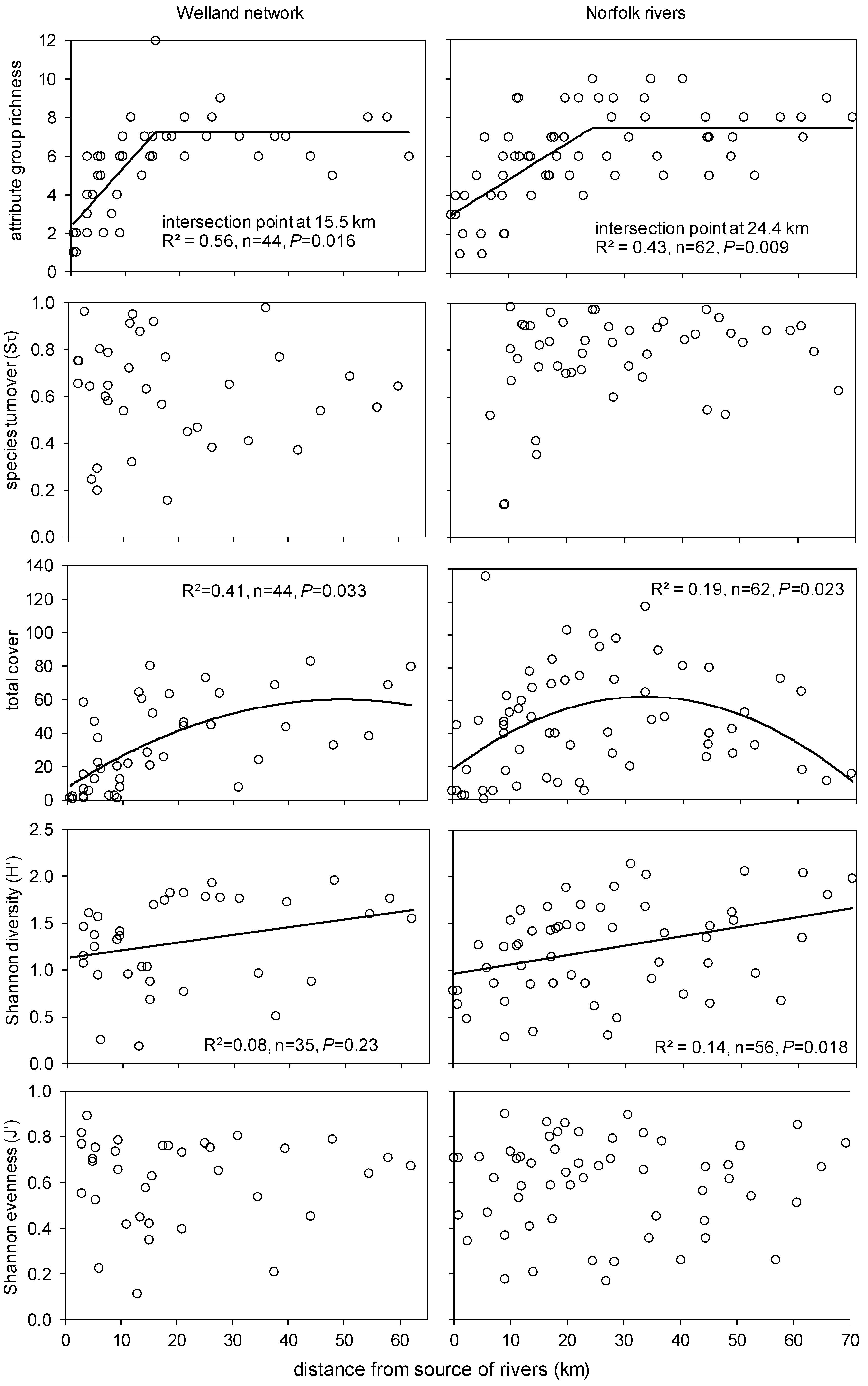
3.4. Spatial Changes along and across River Networks

The patterns in species richness along the distance gradient were similar between the two rivers but very different for hydrophytes and helophytes (Figure 10). Hydrophyte richness increased along the river gradient especially in the headwaters. Helophyte richness remained largely unchanged all along the rivers. These patterns were virtually identical even after correcting for the small differences in sampling area for hydrophytes and river reach length for helophytes. These patterns also held for species richness across the river network (Figure 11). Since the same patterns in species richness and abundance-occurrence were founds in both networks as well as the striking differences between hydrophytes and helophytes, the remaining analyses focus on hydrophytes.

Figure 10. Changes in species richness for hydrophytes and helophytes (marginal plants) as a function of distance from source.

Figure 10. Changes in species richness for hydrophytes and helophytes (marginal plants) as a function of distance from source.

Figure 11. Changes in hydrophyte (square symbols, continuous regression line) and helophytes (triangle symbols, dashed regression line) species richness across river networks.

Figure 11. Changes in hydrophyte (square symbols, continuous regression line) and helophytes (triangle symbols, dashed regression line) species richness across river networks.

Hydrophyte mean local abundance increased with range size along rivers and across networks (Figure 12). Hydrophyte mean local abundance was not however statistically better related to occurrence (range size) along rivers than across entire networks (P = 0.53 for Welland, P = 0.63 for Norfolk datasets). The rate of increase in local abundance against occurrence (correlation slope) was also not statistically different along rivers than across entire networks (P = 0.24 for Welland, P = 0.13 for Norfolk datasets).

Figure 12. Abundance range size relationships across networks (a,c) and along rivers (b,d) for the Welland (a,b) and Norfolk/Wensum (c,d) catchments.

Figure 12. Abundance range size relationships across networks (a,c) and along rivers (b,d) for the Welland (a,b) and Norfolk/Wensum (c,d) catchments.

Local resources (depth, substrate) known to affect hydrophyte composition in the River Wensum were not spatially autocorrelated along the river. The spatial autocorrelation of hydrophyte species composition along rivers was positive for distance intervals up to 10 km (Figure 13). This spatial autocorrelation disappeared however after taking into account the effect of local resources (depth, substrate) on hydrophyte composition. The same analyses run on presence-absence (rather than transformed abundance) showed a stronger pattern: positive autocorrelation at distances up to 10km and negative autocorrelation at long distance intervals (35–45 km). The negative autocorrelation disappeared after taking into account the effect of local resources (depth, substrate) on hydrophyte composition, but positive autocorrelation remain at the shortest distance interval (<5 km). Similar patterns were detected across the networks (Figure 13).

An interesting range of patterns of hydrophyte community structure emerged against distance from source (Figure 14). Attribute group richness increased up to eight attribute groups down to 15 and 24 km from source in the Welland and Norfolk rivers, respectively. Total cover was maximal half way up the distance from source only in Norfolk. Shannon diversity increased linearly with distance but species turnover and species evenness showed no distinctive patterns.

Similar linear relationships existed with depth and width for species and attribute group richness due to collinearity with distance from source, even in Norfolk with 0.19 < r² < 0.42.

Figure 13. Spatial autocorrelation in species composition along rivers and across networks based on log transformed abundance data (square symbols, black line) and presence-absence data (diamond symbols, dashed line). Significant tests are indicated by a filled symbol (after progressive Bonferroni correction of α = 0.05/k for the kth distance class). Positive Mantel statistics represent positive autocorrelation. Mantel statistics range from −1 to 1. Number of comparisons per class was relatively low for the rivers Welland (13–21) and Wensum (20–47) and relatively high for the network analyses (Welland 30–245, Norfolk 83–309).

Figure 13. Spatial autocorrelation in species composition along rivers and across networks based on log transformed abundance data (square symbols, black line) and presence-absence data (diamond symbols, dashed line). Significant tests are indicated by a filled symbol (after progressive Bonferroni correction of α = 0.05/k for the kth distance class). Positive Mantel statistics represent positive autocorrelation. Mantel statistics range from −1 to 1. Number of comparisons per class was relatively low for the rivers Welland (13–21) and Wensum (20–47) and relatively high for the network analyses (Welland 30–245, Norfolk 83–309).

Figure 14. Changes in community structure against distance from source.

Figure 14. Changes in community structure against distance from source.

4. Discussion

4.1. Sampling Design

The river survey over a representative reach scale, here about 50 m long or 500 m², allowed us to record about 3/4 of hydrophyte species but only about 2/3 of helophyte species encountered over 1 km length of river [54]. Long reaches (0.5–1 km, e.g., [36]) allowed the characterization of the vegetation for conservation purposes and large scale mapping but plants could not be related to physical parameters in lowland rivers due to spatial heterogeneity [94].

Whether one uses percentage cover estimate or line transects with quadrats (point frequency), does not make a huge difference in lowland rivers [95], although the latter tends to overlook rare species with low abundance [96]. The key is to have a sufficient number of quadrats per site, such as in e.g. Bornette and Amoros [97] and Riis and Sand-Jensen [41], with at least one hundred 0.25 m × 0.25 m quadrats along transects. Recent examples of inappropriate sampling and difficulties in comparing datasets with different survey designs in long term studies include Martins et al. [98], with only three to nine 1 m² quadrat per site on top of plant patches, and Steffen et al. [99] with exclusion of marginal areas and multiple survey designs. Great care is needed both in species identification and data analyses (e.g., [42]). The survey in the Welland [61] had mis-identifications in Callitriche and Ranunculus corrected for in the present study.

For the long term survey, sites were selected to represent the upper, middle and lower sections of the two rivers. The degree of independence may now be better judged from the spatial autocorrelation analyses of the English rivers. For the spatial studies, great care in data analyses and reporting of probabilities is needed due to the non-independence of study sites along rivers. Probabilities for simple (one outlet, River Welland) river networks are complicated to derive (see [91]) and even more so in the case of complex networks (several outlets, Norfolk rivers).

4.2. Edge Effect: Necessity or Artefact?

The area sampled included all plants rooted (or floating) in water. This is important as marginal plants can facilitate the presence of hydrophytes, especially non-anchored species [35,100]. There will always be a grey area in defining hydrophytes from marginal plants (helophytes) and this may change from region to region or from one end of an environmental gradient to another (e.g., pCO₂, [65]). So it is important to provide species lists. Species lists are also important if we are to interpret absence, as lack of evidence is not evidence of absence [36].

This study provides evidence that marginal plants (helophytes) do not behave in the same way as hydrophytes both in time and space (Figure 3, Figure 4, Figure 6, Figure 10 and Figure 11). In order to compare the number of species between sites along a river, the sampling area was about 500 m². Effectively as the river becomes wider, the marginal area along the river becomes smaller relative to the in-channel area. Because abundance is assessed over the whole area, abundance of marginal plants cannot be as high as in-stream hydrophytes, hence the sampling bias (edge effect). The longitudinal pattern of decreasing helophyte species richness with distance from source may result from this edge effect. Riparian plant studies (rooted above mean water level) generally report increasing species richness with distance from source at least down to the middle of the river [89,90]. Hence this study focused on hydrophytes as in Demars and Harper [43]. Similarly however, the headwaters (<10 km distance from source) may have relatively few hydrophytes because of helophyte encroachment.

4.3. Long Term Changes: Climate, Management Practices and Biotic Interactions

While in-channel aquatic plant biomass or cover has been related to hydrology in previous studies [101,102], this is the first study to link species and species traits, both in composition and richness, to changes in climate (temperature and hydrology). Worryingly, our results showed that climate change (increasing summer low flows, change in winter NAO and winter ice scouring) was related to decreasing richness. This shift in the type and seasonality of disturbance affected mostly amphibious species, reproductive output and phenology.

Change in riparian management led to an increase in shading at two sites and this contributed to change in species composition, decrease in species cover and species (attribute) richness. Weed cutting has long been shown to affect aquatic vegetation [83,103,104,105], but we could not find any significant effects on any of the response variables. Generally it decreased in the Lethe and increased in the Delme, but the records were probably too sporadic at individual sites. Since the water quality (pH, alkalinity, nitrogen, phosphorus) of both rivers remained largely unchanged during the study period [60], it was not possible to quantify its effect.

There are many complex co-evolving biotic interactions [106,107,108]. We only tested here for the effect of green algae cover on vascular plants. With green algae exceeding 10% cover in only 7% of our surveys, it is not surprising that no significant effects on species composition and community structure were detected over the 21 years.

4.4. Short Term Temporal Changes

The result of hydrophyte autocorrelation analyses was as expected from previous studies [24,54,70,109,110,111]. It confirms that hydrophyte regeneration power is relatively high in river system over a short period of time [50,112,113,114]. Nonetheless, annual species turnovers of 0.2–0.4 in the German and English lowland rivers were surprisingly high and this impacted our assessment of richness across temporal scales (Figure 9) as previously found in arid rivers [37]. In the German rivers, species richness was on average 23% and 34% higher over 3 and 5 years, respectively, than over a one year survey. Similarly, in the River Wensum, species richness was 18% higher over three years than over a one year survey. The much lower values for annual species turnover presented in Demars [57] were wrong due to calculation errors. Our perception of short term (1–5 years) plant dynamics and its impact on species richness estimates in lowland rivers is therefore considerably altered.

4.5. Long Term Temporal Changes

While the deterministic exogenous factors reviewed above could explain 19%–34% of the variability in species and species trait hydrophyte composition and richness, time generally explained an additional proportion of the remaining variability. Additionally, the temporal autocorrelations showed an underlying gradient, with unexpected negative values at long time lags even after taking out the effect of exogenous factors. This was due to major shifts in vegetation composition, clearly visible on the multivariate plots. These shifts did not happened synchronously, and after inspection of the raw data, the extreme high flow events of 1985 might have been responsible for the shift in vegetation at Lethe 9 but we could not explain the possible cause for the other sites. This hints at possible stochastic effects (see Figure 5) which are difficult to predict. That said, D10 with only one dominant species (S. emersum) and very few other hydrophyte species, showed possible early signs of a catastrophic crash (large swing in annual species turnover and evenness, see [115]). The underlying mechanisms could be an erosion of the species pool or a change in the longitudinal dispersal due to increased upstream disturbance.

4.6. Spatial Connectivity

The spatial connectivity of the sites could have been studied using other approaches such as a binary coded river network [43,80] or calculating the distances between sites using the shortest river path and additional (arbitrary) distances between river mouths, as the Norfolk rivers are disconnected (e.g., [116]). Here, distances along the river were reflecting probable dispersal by water current and fish, while the shortest distance over land between sites was more appropriately reflecting wind, bird and human dispersal.

There was a very high level of congruence between the two main stems (Welland, Wensum) and river networks studied, as well as between rivers and network analyses. Patterns observed at individual sites were similar to those based on sites grouped by distance from source (Figure 10 and Figure 11), with higher species richness across the network probably due to isolation (cf. Figure 10 and Figure 11). Species and trait diversity increased in the Welland down to about 15–20 km from the source and then remained the same (down to 60 km). In the Norfolk rivers, species trait diversity increased down to about 24 km while species richness continued to increase from source to mouth despite a peak in total cover half way down the river. This provides evidence that either there is a long term in-situ regeneration of taxa (relict from the past, [41]) or continuous dispersal (immigration) from upstream reaches [43] or lateral aquatic habitats (backwaters, standing waters, [117]). There was no evidence of a river domain effect as has been found for riparian plants [59]. Evenness was unrelated to distance from source but surprisingly very variable in contrast to Demars [57]. This was due to the bias in Demars [57] of using Braun-Blanquet scale as opposed to the more appropriate percentage cover scale used in the present study.

The species turnover was highly variable and extremely high, especially in the Norfolk rivers, where efforts were made to sample immediately upstream and downstream of weirs as well as along the whole river. The spatial turnover over an average 3.9 ± 0.3 and 3.2 ± 0.3 km in the Welland and Norfolk networks was generally between 0.4 and 0.9 compared to 0.2 and 0.4 in the inter-annual species turnover. Species composition was not autocorrelated after taking into account exogenous factors (depth, substrate), except for presence-absence of species in the shortest distance class (0–5 km). This provides weak support for dispersal and stronger support for regeneration capacity. The river versus network comparison (Figure 12 and Figure 13) did not provide support for higher dispersal along the water current than across land mass. A re-analysis of the data published in Riis and Sand-Jensen [41], based on the same statistical methods used in this study, showed that neither the correlation coefficient (r) nor the size effect (slope) of the local abundance of strictly submerged and amphibious species against their range (% occurrence) was different from each other’s (P > 0.8) or from all species (P > 0.5). Hence, contrary to the inference of Riis and Sand-Jensen [41], amphibious plants were not shown to disperse more effectively than strictly submerged species. From these statistical analyses it is also easy to see that eight out of their 10 individual stream systems would not have a statistically higher coefficient of determination than the overall relationship; hence contrary to the conclusions of Riis and Sand-Jensen [41], there was no evidence to support the metapopulation theory from their data. This may in part be due to a lack of power in the analyses because of the relatively low number of species.

4.7. Implications

While the temporal resolution and spatial connectivity analyses of this study are unprecedented, the results suggest that larger scales are needed to increase the number of species and integrate the regional species pool. The change in species and attribute compositions over the 21 years period due to the additional effect of time may result from an erosion of the regional species pool [99].

Temporal and spatial autocorrelation analyses indicated that long term hydrophyte biomonitoring, for the Water Framework Directive in lowland rivers, may be carried out at 4–6 years intervals for every 10 km of rivers (Figure 6 and Figure 13). This would be sufficient to characterise changes in hydrophytes, as in current long term studies (e.g., [118,119]). However, a network of representative sites (e.g., in the UK: AWMN, [120]; ECN, [121]) should be surveyed yearly or biannually in order to gain enough statistical power to detect possible underlying causes of hydrophyte changes. Here, the 21 consecutive years gave us enough power to detect significant relationships across the six sites, but the power was not sufficient to analyse data site by site, where only large size effect (>25%) could be detected statistically.

The role of longitudinal connectivity in river networks is gaining momentum in conservation [122,123] and restoration [124,125] yet support for its role in those highly managed rivers, independently of other exogenous factors, was surprisingly weak (Figure 12). This may point to the role of small weirs in preventing longitudinal dispersion of propagules. Further studies should endeavour to carry out comparative studies in more natural rivers as for riparian plants, e.g. [45,126].

In large river basins, tributaries can have relatively low species diversity due to isolation. Species dispersal down the stream tends to increase the diversity of the main stem, at least near confluences [40,127,128,129]. This may in part be due to higher resource heterogeneity [130]. Independently of the spatial structure, richness is otherwise predicted to peak at intermediate spatial heterogeneity and temporal variability [31,131], two exogenous gradients constraining the distribution of species traits [132,133].

Here, as in many studies [32,40], we used an inductive approach to try to explain what might have happened. More specific predictions at the level of traits (e.g., trade-offs) or combination of attributes could be tested experimentally (e.g., [23,53,113,134,135,136]). A more mechanistic and experimental approach could lead to more predictive species distribution and associated community structure against our changing climate and management practices [34,137].

5. Conclusions

Hydrophytes and marginal plants (helophytes) behaved very differently, not just as predicted in species richness (H6) but also in percentage cover, seasonal and long term temporal autocorrelation. Although field surveys of aquatic plants must include marginal areas, patterns in hydrophytes and helophytes are best studied separately. Here, we revisit the hypotheses focusing on general patterns (those replicated across sites) in hydrophytes.

Species and attribute group richness unexpectedly declined over the 21 years record (H5) and responded partly independently of time to winter NAO, number of summer days with low flows and shading (H8). The additional effect of time suggests another underlying gradient (erosion of species pool?) is present (H5). Species and attribute group richness generally increased with distance from source down to 15–25 km to a plateau, except for the Norfolk rivers which showed a continuous increase in species richness all the way down the river mouth despite the low total percentage cover (H6, H7). Evenness was surprisingly very variable and unrelated to distance from source (H7). Annual species turnover was higher than expected and this affected the assessment of species richness across temporal scales; there were many more species recorded over three or five years than over one year (H10).

The seasonal changes in hydrophytes were as predicted (H1). The temporal autocorrelation in species composition (even after removing the effect of exogenous factors) was as predicted: positive at short time lags (high plant regeneration), but unexpectedly negative at several sites at long time lags (H2), due to an unidentified underlying gradient. Most sites showed an unexpected shift in vegetation characterised by two centroids on the multivariate plots.

The spatial turnover was very high (0.4–0.9) over short distances (3–4 km), possibly reflecting the presence of small weirs. The spatial autocorrelation in species composition was surprisingly absent (based on abundance data) or very weak (based on presence-absence data) after removing the effect of exogenous factors (depth, substrate), and not stronger along individual rivers than across entire networks (H3, H4). Species richness against distance from source was similar across spatial scales, i.e., headwaters shared the same species pool, suggesting isolation between head-waters was not very strong (H11). Finally, patterns in abundance range-size were also unexpectedly similar along rivers compared to across entire networks (H12). Altogether, there is only weak evidence for the preponderant role of longitudinal dispersal in structuring plant assemblages. Could this also be the result of the effects of the small weirs?

Over 21 years, the relationships between species traits (attributes) and exogenous factors affecting plant composition were generally very weak, with no strong trade-off but a general erosion of attributes over time attributed to a decrease in winter ice scouring, an increase in shading and summer low flows as well as a remaining effect of time which may be due to an erosion of the regional species pool.

This study has shown that climate change, management and connectivity are all important factors to explain aquatic plant dynamics. Further studies will need to integrate other aquatic habitats along rivers (regional species pool) and larger continental scales to increase the number of species and integrate phylogeny to build a more eco-evolutionary approach. More mechanistic approaches will be necessary to make predictions against our changing climate and management practices.

References

1. Humboldt, A.; Bonpland, A. Essai sur la Géographie des Plantes; Levrault, Schoell et compagnie: Paris, France, 1805. [Google Scholar]
2. Lyell, C. Principles of Geology; John Murray: London, UK, 1830. [Google Scholar]
3. Darwin, C. The Origin of Species by Means of Natural Selection, 6th ed.; John Murray: London, UK, 1872. [Google Scholar]
4. Warming, E. Lehrbuch der ökologischen Pflanzengeographie. Eine Einführung in die Kenntnis der Pflanzenvereine; Gebrüder Bornträger: Berlin, Germany, 1896. [Google Scholar]
5. Hanski, I. Metapopulation dynamics. Nature 1998, 396, 41–49. [Google Scholar] [CrossRef]
6. Moilanen, A.; Hanski, I. On the use of connectivity measures in spatial ecology. Oikos 2001, 95, 147–151. [Google Scholar]
7. Muneepeerakul, R.; Bertuzzo, E.; Lynch, H.J.; Fagan, W.F.; Rinaldo, A.; Rodriguez-Iturbe, I. Neutral metacommunity models predict fish diversity patterns in Mississippi-Missouri basin. Nature 2008, 453, 220–222. [Google Scholar] [CrossRef]
8. Muneepeerakul, R.; Weitz, J.S.; Levin, S.A.; Rinaldo, A.; Rodriguez-Iturbe, I. A neutral metapopulation model of biodiversity in river networks. J. Theor. Biol. 2007, 245, 351–363. [Google Scholar] [CrossRef]
9. Labonne, J.; Ravigne, V.; Parisi, B.; Gaucherel, C. Linking dendritic network structures to population demogenetics: The downside of connectivity. Oikos 2008, 117, 1479–1490. [Google Scholar] [CrossRef]
10. Venail, P.A.; MacLean, R.C.; Bouvier, T.; Brockhurst, M.A.; Hochberg, M.E.; Mouquet, N. Diversity and productivity peak at intermediate dispersal rate in evolving metacommunities. Nature 2008, 452, 210–214. [Google Scholar] [CrossRef]
11. Albert, J.S.; Lovejoy, N.R.; Crampton, W.G.R. Miocene tectonism and the separation of cis- and trans-Andean river basins: Evidence from Neotropical fishes. J. South Am. Earth Sci. 2006, 21, 14–27. [Google Scholar] [CrossRef]
12. Burridge, C.P.; Craw, D.; Waters, J.M. River capture, range expansion, and cladogenesis: The genetic signature of freshwater vicariance. Evolution 2006, 60, 1038–1049. [Google Scholar]
13. Burridge, C.P.; Craw, D.; Waters, J.M. An empirical test of freshwater vicariance via river capture. Mol. Ecol. 2007, 16, 1883–1895. [Google Scholar] [CrossRef]
14. Köhler, F.; Panha, S.; Glaubrecht, M. Speciation and radiation in a river: Assessing the morphological and genetic differentiation in a species flock of viviparous gastropods (Cerithioidea: Pachychilidae). In Evolution in Action; Glaubrecht, M., Ed.; Springer-Verlag Berlin: Heidelberg, Germany, 2010; pp. 513–550. [Google Scholar]
15. Vitule, J.R.S.; Skora, F.; Abilhoa, V. Homogenization of freshwater fish faunas after the elimination of a natural barrier by a dam in Neotropics. Divers. Distrib. 2012, 18, 111–120. [Google Scholar] [CrossRef]
16. April, J.; Hanner, R.H.; Dion-Cote, A.M.; Bernatchez, L. Glacial cycles as an allopatric speciation pump in north-eastern American freshwater fishes. Mol. Ecol. 2013, 22, 409–422. [Google Scholar] [CrossRef]
17. Dias, M.S.; Cornu, J.F.; Oberdorff, T.; Lasso, C.A.; Tedesco, P.A. Natural fragmentation in river networks as a driver of speciation for freshwater fishes. Ecography 2013, 36, 683–689. [Google Scholar] [CrossRef]
18. Hrbek, T.; Ferreira da Silva, V.M.; Dutra, N.; Gravena, W.; Martin, A.R.; Farias, I.P. A new species of river dolphin from Brazil or: How little do we know our biodiversity. PLoS ONE 2014, 9, e83623. [Google Scholar]
19. Jansson, R.; Nilsson, C.; Renofalt, B. Fragmentation of riparian floras in rivers with multiple dams. Ecology 2000, 81, 899–903. [Google Scholar] [CrossRef]
20. Meldgaard, T.; Nielsen, E.E.; Loeschcke, V. Fragmentation by weirs in a riverine system: A study of genetic variation in time and space among populations of European grayling (Thymallus thymallus) in a Danish river system. Conserv. Genet. 2003, 4, 735–747. [Google Scholar] [CrossRef]
21. Jansson, R.; Zinko, U.; Merritt, D.M.; Nilsson, C. Hydrochory increases riparian plant species richness: A comparison between a free-flowing and a regulated river. J. Ecol. 2005, 93, 1094–1103. [Google Scholar] [CrossRef]
22. Raeymaekers, J.A.M.; Raeymaekers, D.; Koizumi, I.; Geldof, S.; Volckaert, F.A.M. Guidelines for restoring connectivity around water mills: A population genetic approach to the management of riverine fish. J. Appl. Ecol. 2009, 46, 562–571. [Google Scholar] [CrossRef]
23. Merritt, D.M.; Nilsson, C.; Jansson, R. Consequences of propagule dispersal and river fragmentation for riparian plant community diversity and turnover. Ecol. Monogr. 2010, 80, 609–626. [Google Scholar] [CrossRef]
24. Butcher, R.W. Studies on the ecology of rivers. I. On the distribution of macrophytic vegetation in the rivers in Britain. J. Ecol. 1933, 21, 58–91. [Google Scholar] [CrossRef]
25. Boedeltje, G.; Bakker, J.P.; Bekker, R.M.; van Groenendael, J.M.; Soesbergen, M. Plant dispersal in a lowland stream in relation to occurrence and three specific life-history traits of the species in the species pool. J. Ecol. 2003, 91, 855–866. [Google Scholar] [CrossRef]
26. Combroux, I.C.S.; Bornette, G. Propagule banks and regenerative strategies of aquatic plants. J. Veg. Sci. 2004, 15, 13–20. [Google Scholar] [CrossRef]
27. Pollux, B.J.A.; Santamaria, L.; Ouborg, N.J. Differences in endozoochorous dispersal between aquatic plant species, with reference to plant population persistence in rivers. Freshwater Biol. 2005, 50, 232–242. [Google Scholar]
28. Gurnell, A.; Goodson, J.; Thompson, K.; Clifford, N.; Armitage, P. The river-bed: A dynamic store for plant propagules? Earth Surf. Proc. Landf. 2007, 32, 1257–1272. [Google Scholar] [CrossRef]
29. Muneepeerakul, R.; Bertuzzo, E.; Rinaldo, A.; Rodriguez-Iturbe, I. Patterns of vegetation biodiversity: The roles of dispersal directionality and river network structure. J. Theor. Biol. 2008, 252, 221–229. [Google Scholar] [CrossRef]
30. Kautsky, L. Life strategies of aquatic soft bottom macrophytes. Oikos 1988, 53, 126–135. [Google Scholar] [CrossRef]
31. Bornette, G.; Henry, C.; Barrat, M.-H.; Amoros, C. Theoretical habitat templets, species traits, and species richness: aquatic macrophytes in the upper Rhone River and its floodplain. Freshwater Biol. 1994, 31, 487–505. [Google Scholar] [CrossRef]
32. Mouw, J.E.B.; Alaback, P.B. Putting floodplain hyperdiversity in a regional context: An assessment of terrestrial-floodplain connectivity in a montane environment. J. Biogeogr. 2003, 30, 87–103. [Google Scholar] [CrossRef]
33. Merritt, D.M.; Scott, M.L.; Poff, N.L.; Auble, G.T.; Lytle, D.A. Theory, methods and tools for determining environmental flows for riparian vegetation: Riparian vegetation-flow response guilds. Freshwater Biol. 2010, 55, 206–225. [Google Scholar] [CrossRef]
34. Greet, J.; Webb, J.A.; Cousens, R.D. The importance of seasonal flow timing for riparian vegetation dynamics: A systematic review using causal criteria analysis. Freshwater Biol. 2011, 56, 1231–1247. [Google Scholar] [CrossRef]
35. Haslam, S.M. River Plants; Cambridge University Press: Cambridge, UK, 1978. [Google Scholar]
36. Holmes, N.T.H. Typing British Rivers according to Their Flora; Nature Conservancy Council: Shrewsbury, UK, 1983. [Google Scholar]
37. Katz, G.L.; Denslow, M.W.; Stromberg, J.C. The Goldilocks effect: Intermittent streams sustain more plant species than those with perennial or ephemeral flow. Freshwater Biol. 2012, 57, 467–480. [Google Scholar] [CrossRef]
38. Holmes, N.T.H.; Whitton, B.A. Submerged bryophytes and angiosperms of the River Tweed and its tributaries. Trans. Bot. Soc. Edinb. 1975, 42, 383–395. [Google Scholar] [CrossRef]
39. Haury, J. Patterns of macrophyte distribution within a breton brook compared with other study scales. Landsc. Urban Plan. 1995, 31, 349–361. [Google Scholar] [CrossRef]
40. Honnay, O.; Verhaeghe, W.; Hermy, M. Plant community assembly along dendritic networks of small forest streams. Ecology 2001, 82, 1691–1702. [Google Scholar] [CrossRef]
41. Riis, T.; Sand-Jensen, K. Abundance-range size relationships in stream vegetation in Denmark. Plant Ecol. 2002, 161, 175–183. [Google Scholar] [CrossRef]
42. Riis, T.; Sand-Jensen, K. Historical changes in species composition and richness accompanying perturbation and eutrophication of Danish lowland streams over 100 years. Freshwater Biol. 2001, 46, 269–280. [Google Scholar] [CrossRef]
43. Demars, B.O.L.; Harper, D.M. Distribution of aquatic vascular plants in lowland rivers: Separating the effects of local environmental conditions, longitudinal connectivity and river basin isolation. Freshwater Biol. 2005, 50, 418–437. [Google Scholar] [CrossRef]
44. Gornall, R.J.; Hollingsworth, P.M.; Preston, C.D. Evidence for spatial structure and directional gene flow in a population of an aquatic plant, Potamogeton coloratus. Heredity 1998, 80, 414–421. [Google Scholar] [CrossRef]
45. Andersson, E.; Nilsson, C.; Johansson, M.E. Effects of river fragmentation on plant dispersal and riparian flora. Regul. Rivers Res. Manag. 2000, 16, 83–89. [Google Scholar] [CrossRef]
46. Boedeltje, G.; Bakker, J.P.; Ten Brinke, A.; Van Groenendael, J.M.; Soesbergen, M. Dispersal phenology of hydrochorous plants in relation to discharge, seed release time and buoyancy of seeds: The flood pulse concept supported. J. Ecol. 2004, 92, 786–796. [Google Scholar] [CrossRef]
47. Pollux, B.J.A.; Jong, M.D.E.; Steegh, A.; Verbruggen, E.; Van Groenendael, J.M.; Ouborg, N.J. Reproductive strategy, clonal structure and genetic diversity in populations of the aquatic macrophyte Sparganium emersum in river systems. Mol. Ecol. 2007, 16, 313–325. [Google Scholar]
48. Pollux, B.J.A.; De Jong, M.; Steegh, A.; Ouborg, N.J.; Van Groenendael, J.M.; Klaassen, M. The effect of seed morphology on the potential dispersal of aquatic macrophytes by the common carp (Cyprinus carpio). Freshwater Biol. 2006, 51, 2063–2071. [Google Scholar] [CrossRef]
49. Fer, T.; Hroudova, Z. Detecting dispersal of Nuphar lutea in river corridors using microsatellite markers. Freshwater Biol. 2008, 53, 1409–1422. [Google Scholar] [CrossRef]
50. Henry, C.P.; Amoros, C.; Bornette, G. Species traits and recolonization processes after flood disturbances in riverine macrophytes. Vegetatio 1996, 122, 13–27. [Google Scholar] [CrossRef]
51. Barrat-Segretain, M.H.; Bornette, G. Regeneration and colonization abilities of aquatic plant fragments: Effect of disturbance seasonality. Hydrobiologia 2000, 421, 31–39. [Google Scholar] [CrossRef]
52. Puijalon, S.; Piola, F.; Bornette, G. Abiotic stresses increase plant regeneration ability. Evol. Ecol. 2008, 22, 493–506. [Google Scholar] [CrossRef]
53. Gurnell, A.; Thompson, K.; Goodson, J.; Moggridge, H. Propagule deposition along river margins: Linking hydrology and ecology. J. Ecol. 2008, 96, 553–565. [Google Scholar] [CrossRef]
54. Wiegleb, G. Recherches Méthodologiques sur les Groupemnents Végétaux des Eaux Courantes. In Colloques Phytosociologiques X. Les Végétations Aquatiques et Amphibies 1981; Koeltz Scientific Books: Lille, France, 1983; pp. 69–83. [Google Scholar]
55. Tremp, H. Spatial and environmental effects on hydrophytic macrophyte occurrence in the Upper Rhine floodplain (Germany). Hydrobiologia 2007, 586, 167–177. [Google Scholar] [CrossRef]
56. Pedersen, T.C.M.; Baattrup-Pedersen, A.; Madsen, T.V. Effects of stream restoration and management on plant communities in lowland streams. Freshwater Biol. 2006, 51, 161–179. [Google Scholar] [CrossRef]
57. Demars, B.O.L. Aquatic Vascular Plants in Nitrate-Rich Calcareous Lowland Streams: Do They Respond to Phosphorus Enrichment and Control? Ph.D. Thesis, University of Leicester, Leicester, UK, 2002. [Google Scholar]
58. Wiegleb, G. A study of habitat conditions of the macrophytic vegetation in selected river systems in western lower saxony (Federal Republic of Germany). Aquat. Bot. 1984, 18, 313–352. [Google Scholar] [CrossRef]
59. Dunn, R.R.; Colwell, R.K.; Nilsson, C. The river domain: Why are there more species halfway up the river? Ecography 2006, 29, 251–259. [Google Scholar] [CrossRef]
60. Wiegleb, G.; Herr, W.; Todeskino, D. Ten years of vegetation dynamics in two rivulets in Lower Saxony (FRG). Vegetatio 1989, 82, 163–178. [Google Scholar] [CrossRef]
61. Demars, B.O.L.; Harper, D.M. The aquatic macrophytes of an English lowland river system: Assessing response to nutrient enrichment. Hydrobiologia 1998, 384, 75–88. [Google Scholar] [CrossRef]
62. Clarke, A.; Nally, R.M.; Bond, N.; Lake, P.S. Macroinvertebrate diversity in headwater streams: A review. Freshwater Biol. 2008, 53, 1707–1721. [Google Scholar] [CrossRef]
63. Legendre, P. Spatial autocorrelation: Trouble or new paradigm? Ecology 1993, 74, 1659–1673. [Google Scholar] [CrossRef]
64. Tremp, H. Geostatistische Analyse der Strahlwirkung in Fließgewässern am Beispiel der Wasserpflanzen. In der Deutsche Gesellschaft für Limnologie (DGL), Erweiterte Zusammenfassungen der Jahrestagung 2008; Hardegsen: Konstanz, Germany, 2009; pp. 518–523. [Google Scholar]
65. Demars, B.O.L.; Trémolières, M. Aquatic macrophytes as bioindicators of carbon dioxide in groundwater fed rivers. Sci. Total. Environ. 2009, 407, 4752–4763. [Google Scholar] [CrossRef]
66. Borcard, D.; Legendre, P.; Drapeau, P. Partialling out the spatial component of ecological variation. Ecology 1992, 73, 1045–1055. [Google Scholar] [CrossRef]
67. Lennon, J.J.; Koleff, P.; Greenwood, J.J.D.; Gaston, K.J. Contribution of rarity and commonness to patterns of species richness. Ecol. Lett. 2004, 7, 81–87. [Google Scholar]
68. Willby, N.J.; Abernethy, V.J.; Demars, B.O.L. An attribute-based classification of European hydrophytes and its relationship to habitat utilisation. Freshwater Biol. 2000, 43, 43–74. [Google Scholar] [CrossRef]
69. Wiegleb, G.; Bröring, U.; Filetti, M.; Brux, H.; Herr, W. Long-term dynamics of macrophyte dominance and growth form types in two Northwest German lowland streams. Freshwater Biol. 2014, 59. [Google Scholar] [CrossRef]
70. Dawson, H.F.; Castellano, E.; Ladle, M. Concept of species succession in relation to river vegetation and management. Verh. Internat. Verein. Limnol. 1978, 20, 1429–1434. [Google Scholar]
71. Walter, R.C.; Merritts, D.J. Natural streams and the legacy of water-powered mills. Science 2008, 319, 299–304. [Google Scholar] [CrossRef]
72. Demars, B.O.L. Using Aquatic Macrophytes for Assessing Water Trophic Level in a Lowland River System. Master’s Thesis, Leicester University, Leicester, UK, 1996. [Google Scholar]
73. Pope, A. GB rivers. Available online: http://hdl.handle.net/10672/85 (accessed on 28 November 2013).
74. Ordnance Survey OpenData™. Available online: https://www.ordnancesurvey.co.uk/ opendatadownload/products.html (accessed on 16 November 2012).
75. Holmes, N.T.H. The Use of Riverine Macrophytes for the Assessment of Trophic Status: Review of 1994/95 Data & Refinements for Future Use; Report to the National Rivers Authority Anglian Region; National Rivers Authority: Peterborough, Canada, 1996. [Google Scholar]
76. Holmes, N.T.H.; Newman, J.R.; Chadd, S.; Rouen, K.J.; Saint, L.; Dawson, F.H. Mean Trophic Rank: A User’s Manual; Report number E38; Environment Agency: Bristol, UK, 1999; pp. 1–133. [Google Scholar]
77. Blanquet, J.B. Plant Sociology: The Study of Plant Communities, 1st ed.; Mc Graw Hill Book Co: New York, NY, USA, 1932. [Google Scholar]
78. Ter Braak, C.J.F.; Šmilauer, P. CANOCO Reference Manual and Canodraw for Windows User’s Guide: Software for Canonical Community Ordination (version 4.5); Microcomputer Power: Ithaca, NY, USA, 2002. [Google Scholar]
79. GenStat. VSN International. Available online: http://www.vsni.co.uk/software/genstat (accessed on 1 April 2014).
80. Legendre, P.; Legendre, L. Numerical Ecology; Elsevier Science: Amsterdam, the Netherland, 1998. [Google Scholar]
81. Tokeshi, M. Niche apportionment or random assortment: Species abundance patterns revisited. J. Anim. Ecol. 1990, 59, 1129–1146. [Google Scholar] [CrossRef]
82. Baattrup-Pedersen, A.; Larsen, S.E.; Riis, T. Long-term effects of stream management on plant communities in two Danish lowland streams. Hydrobiologia 2002, 481, 33–45. [Google Scholar] [CrossRef]
83. Baattrup-Pedersen, A.; Larsen, S.E.; Riis, T. Composition and richness of macrophyte communities in small Danish streams—Influence of environmental factors and weed cutting. Hydrobiologia 2003, 495, 171–179. [Google Scholar] [CrossRef]
84. Arthington, A.H.; Naiman, R.J.; McClain, M.E.; Nilsson, C. Preserving the biodiversity and ecological services of rivers: New challenges and research opportunities. Freshwater Biol. 2010, 55, 1–16. [Google Scholar]
85. Monthly Teleconnection Index: North Atlantic Oscillation (NAO). Available online: ftp://ftp.cpc.ncep.noaa.gov/wd52dg/data/indices/nao_index.tim (accessed on 1 April 2014).
86. Legendre, P.; Galzin, R.; Harmelin-Vivien, M.L. Relating behavior to habitat: Solutions to the fourth-corner problem. Ecology 1997, 78, 547–562. [Google Scholar]
87. Gould, S.J.; Lewontin, R.C. The spandrels of San Marco and the Panglossian paradigm: A critique of the adaptationist programme. Proc. R. Soc Lond. Ser. B Biol. Sci. 1979, 205, 581–598. [Google Scholar] [CrossRef]
88. Holmes, N.T.H.; Whitton, B.A. Macrophytes of the River Tweed. Trans. Bot. Soc. Edinb. 1975, 42, 369–381. [Google Scholar] [CrossRef]
89. Nilsson, C.; Grelsson, G.; Johansson, M.; Sperens, U. Patterns of plant species richness along riverbanks. Ecology 1989, 70, 77–84. [Google Scholar] [CrossRef]
90. Décamps, H.; Tabacchi, E. Species richness in vegetation along river margins. In Aquatic Ecology: Scale, Pattern and Process; Giller, P.S., Hildrew, A., Raffaelli, D.G., Eds.; Blackwell Science: Oxford, UK, 1994. [Google Scholar]
91. Peterson, E.E.; Hoef, J.M.V. A mixed-model moving-average approach to geostatistical modeling in stream networks. Ecology 2010, 91, 644–651. [Google Scholar] [CrossRef]
92. Wuensch, K.L. Comparing correlation coefficients, slopes, and intercepts. Statistics Lessons. Available online: http://core.ecu.edu/psyc/wuenschk/statslessons.htm (accessed on 13 November 2013).
93. Beyer, H.L. Geospatial Modelling Environment, Available online:. Available online: http://www.spatialecology.com/gme/ (accessed on 10 October 2013).
94. Demars, B.O.L.; Edwards, A.C. Distribution of aquatic macrophytes in contrasting river systems: A critique of compositional-based assessment of water quality. Sci. Total. Environ. 2009, 407, 975–990. [Google Scholar] [CrossRef]
95. Scott, W.A.; Adamson, J.K.; Rollinson, J.; Parr, T.W. Monitoring of aquatic macrophytes for detection of long-term change in river systems. Environ. Monit. Assess 2002, 73, 131–153. [Google Scholar] [CrossRef]
96. Daniel, H. Evaluation de la Qualité des cours d’eau par la Végétation Macrophytique. Travail in situ et Expérimental Dans le Massif Armoricain sur les Pollutions par les Macronutriments. Ph.D. Thesis, Ecole Nationale Supérieure Agronomique de Rennes, Rennes, France, 1998. [Google Scholar]
97. Bornette, G.; Amoros, C. Aquatic vegetation and hydrology of a braided river floodplain. J. Veg. Sci. 1991, 2, 497–512. [Google Scholar] [CrossRef]
98. Martins, S.V.; Milne, J.; Thomaz, S.M.; McWaters, S.; Mormul, R.P.; Kennedy, M.; Murphy, K. Human and natural drivers of changing macrophyte community dynamics over 12 years in a Neotropical riverine floodplain system. Aquat. Conserv. Mar. Freshw. Ecosyst. 2013, 23, 678–697. [Google Scholar]
99. Steffen, K.; Becker, T.; Herr, W.; Leuschner, C. Diversity loss in the macrophyte vegetation of northwest German streams and rivers between the 1950s and 2010s. Hydrobiologia 2013, 713, 1–17. [Google Scholar] [CrossRef]
100. Breugnot, E.; Dutartre, A.; Laplace-Treyture, C.; Haury, J. Local distribution of macrophytes and consequences for sampling methods in large rivers. Hydrobiologia 2008, 610, 13–23. [Google Scholar] [CrossRef]
101. Wilby, R.L.; Cranston, L.E.; Darby, E.J. Factors governing macrophyte status in Hampshire chalk streams: Implications for catchment management. J. Chart. Inst. Water and Environ. Manag. 1998, 12, 179–187. [Google Scholar] [CrossRef]
102. Sosiak, A. Long-term response of periphyton and macrophytes to reduced municipal nutrient loading to the Bow River (Alberta, Canada). Can. J. Fish Aquat. Sci. 2002, 59, 987–1001. [Google Scholar] [CrossRef]
103. Soulsby, P.G. The effect of a heavy cut on the subsequent growth of aquatic plants in a Hampshire chalk stream. J. Inst. Fish. Manag. 1974, 5, 49–53. [Google Scholar]
104. Ham, S.F.; Wright, J.F.; Berrie, A.D. The effect of cutting on the growth and recession of the freshwater macrophyte Ranunculus penicillatus (Dumort.) Bab. var. calcareus (R.W. Butcher) C.D.K. Cook. J. Environ. Manag. 1982, 15, 263–271. [Google Scholar]
105. Fox, A.M.; Murphy, K.J. The efficacy and ecological impacts of herbicide and cutting regimes on the submerged plant communities of four British rivers. I. Comparison of management efficacies. J. Appl. Ecol. 1990, 27, 520–540. [Google Scholar] [CrossRef]
106. Parker, J.D.; Burkepile, D.E.; Collins, D.O.; Kubanek, J.; Hay, M.E. Stream mosses as chemically-defended refugia for freshwater macroinvertebrates. Oikos 2007, 116, 302–312. [Google Scholar] [CrossRef]
107. Rybicki, N.B.; Landwehr, J.M. Long-term changes in abundance and diversity of macrophyte and waterfowl populations in an estuary with exotic macrophytes and improving water quality. Limnol. Oceanogr. 2007, 52, 1195–1207. [Google Scholar] [CrossRef]
108. Elger, A.; Willby, N.J.; Cabello-Martinez, M. Invertebrate grazing during the regenerative phase affects the ultimate structure of macrophyte communities. Freshwater Biol. 2009, 54, 1246–1255. [Google Scholar] [CrossRef]
109. Haury, J.; Aidara, L.G. Macrophyte cover and standing crop in the River scorff and its tributaries (Brittany, northwestern France): Scale, patterns and process. Hydrobiologia 1999, 415, 109–115. [Google Scholar] [CrossRef]
110. Sand-Jensen, K.; Andersen, K.; Andersen, T. Dynamic properties of recruitment, expansion and mortality of macrophyte patches in streams. Int. Rev. Hydrobiol. 1999, 84, 497–508. [Google Scholar]
111. Champion, P.D.; Tanner, C.C. Seasonality of macrophytes and interaction with flow in a New Zealand lowland stream. Hydrobiologia 2000, 441, 1–12. [Google Scholar] [CrossRef]
112. Barrat-Segretain, M.H.; Amoros, C. Recolonization of cleared riverine macrophyte patches: Importance of the border effect. J. Veg. Sci. 1996, 7, 769–776. [Google Scholar] [CrossRef]
113. Barrat-Segretain, M.H.; Amoros, C. Recovery of riverine vegetation after experimental disturbance: A field test of the patch dynamics concept. Hydrobiologia 1996, 321, 53–68. [Google Scholar] [CrossRef]
114. Kõrs, A.; Vilbaste, S.; Käeiro, K.; Pall, P.; Piirsoo, K.; Truu, J.; Viik, M. Temporal changes in the composition of macrophyte communities and environmental factors governing the distribution of aquatic plants in an unregulated lowland river (Emajogi, Estonia). Boreal Environ. Res. 2012, 17, 460–472. [Google Scholar]
115. Scheffer, M.; Bascompte, J.; Brock, W.A.; Brovkin, V.; Carpenter, S.R.; Dakos, V.; Held, H.; van Nes, E.H.; Rietkerk, M.; Sugihara, G. Early-warning signals for critical transitions. Nature 2009, 461, 53–59. [Google Scholar] [CrossRef]
116. Urban, M.C.; Skelly, D.K.; Burchsted, D.; Price, W.; Lowry, S. Stream communities across a rural-urban landscape gradient. Divers. Distrib. 2006, 12, 337–350. [Google Scholar] [CrossRef]
117. Amoros, C.; Bornette, G. Connectivity and biocomplexity in waterbodies of riverine floodplains. Freshwater Biol. 2002, 47, 761–776. [Google Scholar] [CrossRef]
118. Whitton, B.A.; Boulton, P.N.G.; Clegg, E.M.; Gemmell, J.J.; Graham, G.G.; Gustar, R.; Moorhouse, T.P. Long-term changes in macrophytes of British rivers: 1. River Wear. Sci. Total Environ. 1998, 210/211, 411–426. [Google Scholar] [CrossRef]
119. Schweinitz, P.; Poschlod, P.; Zeltner, G.-H.; Kohler, A. Langzeitmonitoring (1970–2010) zur Verbreitung der Makrophyten im Fließgewässersystem Moosach (Münchner Ebene). In der Deutschen Gesellschaft für Limnologie (DGL), Erweiterte Zusammenfassungen der Jahrestagung 2011; Hardegsen: Weihenstephan, Germany, 2012; pp. 98–103. [Google Scholar]
120. Kernan, M.; Battarbee, R.W.; Curtis, C.J.; Monteith, D.T.; Shilland, E.M. Recovery of Lakes and Streams in the UK from the Effects of Acid Rain UK Acid Waters Monitoring Network 20 Year Interpretative Report; Environmental Change Research Centre: London, UK, 2010. [Google Scholar]
121. UK Environmental Change Network. Available online: http://www.ecn.ac.uk/ (accessed on 1 April 2014).
122. Moilanen, A.; Leathwick, J.; Elith, J. A method for spatial freshwater conservation prioritization. Freshwater Biol. 2008, 53, 577–592. [Google Scholar] [CrossRef]
123. Hermoso, V.; Linke, S.; Prenda, J.; Possingham, H.P. Addressing longitudinal connectivity in the systematic conservation planning of fresh waters. Freshwater Biol. 2011, 56, 57–70. [Google Scholar] [CrossRef]
124. Renöfält, B.M.; Jansson, R.; Nilsson, C. Effects of hydropower generation and opportunities for environmental flow management in Swedish riverine ecosystems. Freshwater Biol. 2010, 55, 49–67. [Google Scholar] [CrossRef]
125. Brederveld, R.J.; Jahnig, S.C.; Lorenz, A.W.; Brunzel, S.; Soons, M.B. Dispersal as a limiting factor in the colonization of restored mountain streams by plants and macroinvertebrates. J. Appl. Ecol. 2011, 48, 1241–1250. [Google Scholar] [CrossRef]
126. Andersson, E.; Nilsson, C.; Johansson, M.E. Plant dispersal in boreal rivers and its relation to the diversity of riparian flora. J. Biogeogr. 2000, 27, 1095–1106. [Google Scholar] [CrossRef]
127. Holmes, N.T.H. The Vegetation of the River Tweed. Ph.D. Thesis, Durham University, Durham, UK, 1975. [Google Scholar]
128. Fernandes, C.C.; Podos, J.; Lundberg, J.G. Amazonian ecology: Tributaries enhance the diversity of electric fishes. Science 2004, 305, 1960–1962. [Google Scholar] [CrossRef]
129. Besemer, K.; Peter, H.; Logue, J.B.; Langenheder, S.; Lindstrom, E.S.; Tranvik, L.J.; Battin, T.J. Unraveling assembly of stream biofilm communities. Isme J. 2012, 6, 1459–1468. [Google Scholar] [CrossRef]
130. Gascon, C.; Smith, M.L. Where rivers meet. Science 2004, 305, 1922–1923. [Google Scholar] [CrossRef]
131. Townsend, C.R. The patch dynamics concept of stream community ecology. J. N. Am. Benthol. Soc. 1989, 8, 36–50. [Google Scholar] [CrossRef]
132. Grime, J.P. Evidence for the existence of three primary strategies in plants and its relevance to ecological and evolutionary theory. Am. Nat. 1977, 111, 1169–1194. [Google Scholar]
133. Townsend, C.R.; Hildrew, A.G. Species traits in relation to a habitat templet for river systems. Freshwater Biol. 1994, 31, 265–275. [Google Scholar] [CrossRef]
134. Johansson, M.E.; Nilsson, C.; Nilsson, E. Do rivers function as corridors for plant dispersal? J. Veg. Sci. 1996, 7, 593–598. [Google Scholar] [CrossRef]
135. Moggridge, H.L.; Gurnell, A.M.; Mountford, J.O. Propagule input, transport and deposition in riparian environments: the importance of connectivity for diversity. J. Veg. Sci. 2009, 20, 465–474. [Google Scholar] [CrossRef]
136. Nilsson, C.; Ekblad, A.; Dynesius, M.; Backe, S.; Gardfjell, M.; Carlberg, B.; Hellqvist, S.; Jansson, R. A comparison of species richness and traits of riparian plants between a main river channel and tributaries. J. Ecol. 1994, 82, 281–295. [Google Scholar] [CrossRef]
137. Buckley, L.B.; Urban, M.C.; Angilletta, M.J.; Crozier, L.G.; Rissler, L.J.; Sears, M.W. Can mechanism inform species’ distribution models? Ecol. Lett. 2010, 13, 1041–1054. [Google Scholar]
138. Stace, C.A. New Flora of the British Isles, 2nd Ed. ed; Cambridge University Press: Cambridge, UK, 1997. [Google Scholar]