Characteristics of Underwater Acoustics in Different Habitat Types along a Natural River Channel

Abstract

Fluvial biological habitat types are classified using the diversity in physical characteristics of a water channel. Recent ecological management studies have highlighted the potential of underwater sound as a quantitative indicator of habitat characteristics. We investigate the relationship between underwater acoustic characteristics and hydraulic factors of 12 habitat types in the Namdae Stream in Yangyang, Korea, namely riffles, pools, and step riffle habitats. In the riffles and pools, the underwater sound levels were measured as sound pressure levels (SPLs). SPL(RMS) and 1/3 octave band have been measured in the frequency range between 8 Hz and 20 kHz. Among riffles, high SPL corresponded to the descending level of flow velocity. Pools generally had a low SPL. Low-frequency sound waves in the upper regions are better transmitted in the deeper water. To quantitatively analyze the water depth and flow velocity, we used a regression between the observed water depth, flow velocity, and acoustic SPL. The application of this study was certificated. The correlation coefficients between SPL and flow velocity/water depth revealed specific frequency bands with very strong positive correlations between SPL and flow rate in riffles and very strong negative correlations between SPL and pool water depth. Consequently, underwater sound can be used as an alternative for evaluating biological habitats.

1. Introduction

Living organisms in natural channels may exist in different aquatic habitats according to the prevailing physical, chemical, and biological, environmental conditions [1,2]. Major factors contributing to the formation of biological aquatic habitats include water flow, light, temperature, substance inflow and transport, and bed slope [3]. Assessing the natural and ecological functions of biological habitats formed by these various factors is very important in understanding the habitat and movement characteristics of underwater organisms [4].

The fish varieties and community assemblages are significantly affected by physical characteristics such as water depth, flow velocity, bed slope, bed substrate, and vegetation [5,6,7,8]. Habitats can be classified into various types by these characteristics, such as pools (where the water depth is relatively deep and flow velocity is slow), riffles (where the water depth is shallow and flow velocity is fast), and step riffles (which have a head, i.e., a difference in elevation). Channel habitats contain various aquatic characteristics and are subject to considerable changes, especially when there is an enormous channel-changing event, such as a flood [4]. The channel environment can also be altered by channel restoration or artificial construction. These factors can significantly change the biological environment. Therefore, technology that can effectively identify modifications to channel habitats using temporal and spatial characteristics is required [4].

Certain physical sounds recorded below the water surface can potentially serve as quantitative indicators of the soundscape of a habitat. Tonolla et al. [9] identified that the flow of water is interrupted by the different hydraulic characteristics of channels, and sounds occur due to the flow velocity, flow rate, and bubbles. Tonolla et al. [9] also reported that the underwater sound pressure increases with the flow velocity. Tonolla et al. [10] identified that different channel types clearly cause different underwater acoustic characteristics, and the ratio of flow velocity to water depth, relative roughness coefficient, and Froude number are the major hydraulic factors explaining the variation. Amoser and Ladich [11] conducted research on the underwater acoustic characteristics of areas with flowing water (such as channels) and static areas (such as lakes) and found the underwater sounds of each area are created by the combination of water flow, transport of bed substrates, wind, animal sounds, and artificial sounds. Therefore, the underwater acoustic characteristics of a channel are significantly affected by the underwater and surrounding environments, as well as the physical characteristics of the channel. Underwater sounds have the potential to be applied as a new method to assess channel environments.

Sounds are not attenuated as quickly as light and chemical substances and can travel far in underwater environments, rendering water a very important signal carrier [12,13,14]. As sounds provide important information on habitats and ecosystems, the auditory senses of aquatic organisms to acquire sound information is very important for their survival [9,15]. Fish are capable of hearing sounds from 50 to 2000 Hz [16]. If fish can analyze sound and be controlled through underwater sounds in this range, these sounds can be good candidates for modifying fish movement against potentially hazardous environments and controlling them for improved fish management [16].

Underwater sounds are created by sound waves, which are pressure disturbances transmitted by water. The energy of sound waves includes the change in local pressure and vibrations in the water. At a specific wavelength and instant, water molecules perform directional motions. This molecular motion becomes a major component of a sound field relatively close to the sound source. At a location relatively far from the sound source, the pressure becomes the major component of a sound field. The distance traveled by molecular motions is the major component of a sound field, and variations depend on the sound frequency and density of the medium. Molecular motions are preserved over a much longer distance in the water, which has a higher density than air. Such molecular motions of sound waves are not important for terrestrial organisms, but they play a very important role in delivering a diverse array of information to aquatic animals [12,16]. For this reason, many recent studies have investigated underwater acoustic characteristics, that is, the sound environment of biological habitats. However, no research has been undertaken in Korea.

In this study, the Namdae Stream in Yangyang, South Korea, was selected for the field research because it has deep valleys and many tributaries. The flow distance is long with an abundant flow volume [17]. It contains a diverse array of representative natural channels and is inhabited by various living organisms. It is surrounded by mountains and forests, and the river valley supports very few human inhabitants and scanty vehicular traffic. It is mostly characterized by a natural sound environment with limited anthropogenic noise. This study investigates the relationship between underwater acoustic characteristics of the Namdae Stream with channel types (riffles, pools, and step riffles) and the hydraulic factors of the channel, such as flow velocity, water depth, and bed substrate. This study compares underwater sound pressure levels (SPLs) using the ratio of water depth to bed substrate size and demonstrates that the SPLs in flowing water are closely related to the flow velocity and flow-interrupting substrates. We sought to employ a better effective approach in characterizing the aquatic ecosystem using underwater acoustic in the habitat.

2. Materials and Methods

2.1. Field Channel and Investigation Method

To analyze the acoustic characteristics of natural channels, the Namdae Stream in Yangyang was selected as the field location because it has a relatively well-preserved natural environment. The Namdae Stream is part of the largest watershed in the Yeongdong Region, with a total reach length of 73.3 km and a catchment area of 232.9 km². It originates in the eastern valley of Duro-bong, Samsan-ri, Yeongok-myeon, and Gangneung City (1422 m). It joins the Hu Stream in Yangyang-eup, and flows into the East Sea in a northeast direction [18,19]. The investigated reaches were located in mountainous regions upstream of the Namdae Stream, encompassing 21.3 km of the waterway and a catchment area of 88.5 km² in Hyeonbuk-myeong. It has a large curvature with the characteristics of a meandering channel composed of riffles, step riffles, and pools.

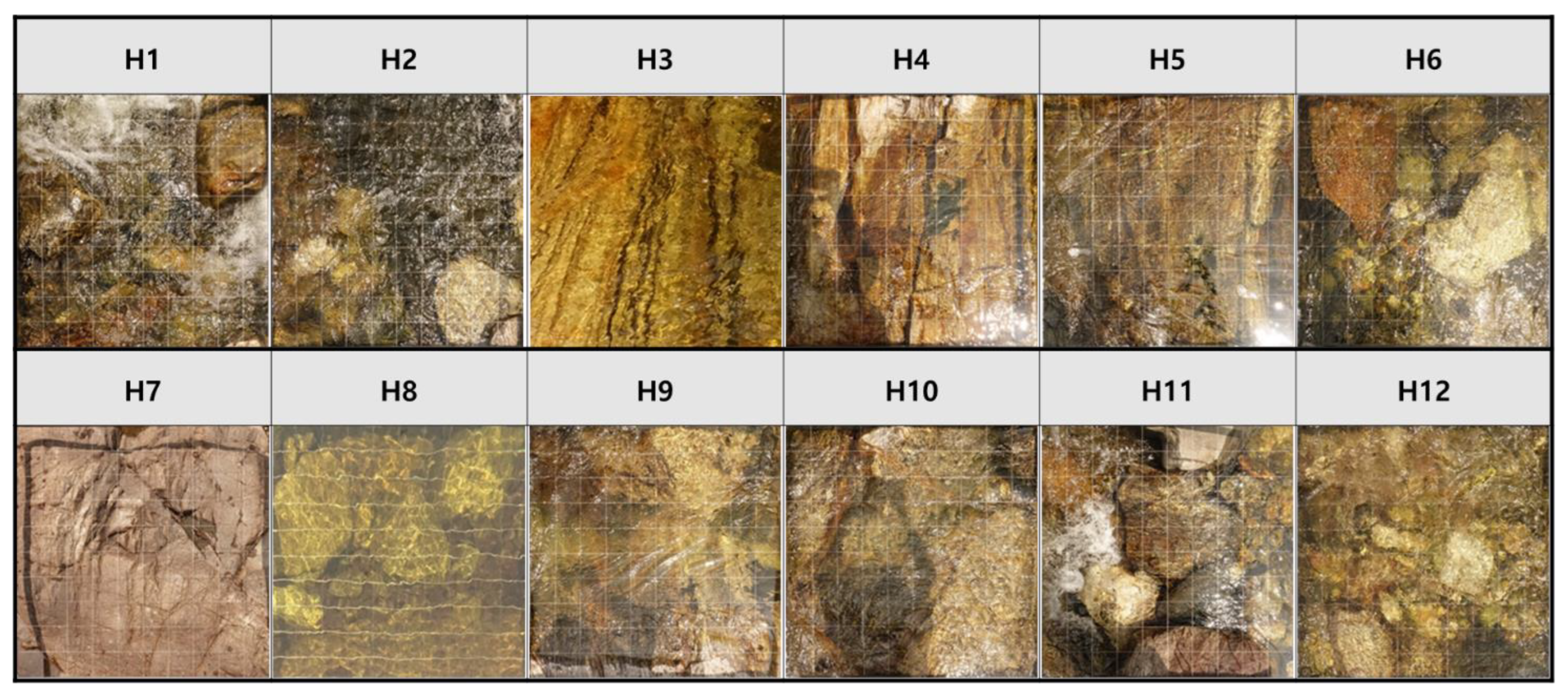
The underwater acoustic characteristics of the natural channel and the physical characteristics of the habitats were analyzed by a field survey (upstream of the Namdae Stream) conducted from 26 to 30 June (before the rainy season). The rainfall recorded in the vicinity of the field channel was used due to a lack of available data taken directly from the channel. The antecedent dry period was 14 days. The mean total precipitation for the month before the survey was 51 mm. The rainfall data used was the mean value during the previous month, which was provided by the Korea meteorological Administration, Korea (KMA) [20]. The average temperature during the period was between 20 °C to 25 °C, with a maximum of 31.4 °C and a minimum of 16.6 °C (KMA) [20]. A total of 12 reaches near the Habshil Bridge in the area upstream of the Namdae Stream in Yangyang were selected as the field sites, as demonstrated in Figure 1. From upstream to downstream, the longitudinal distance of each recording point was measured for the site spacings. The bed structures in each section were identified using the sampling frame and characterized using the sediment size classes of the Wentworth scale [21]. The bed substrate size was determined using a 1 × 1 m square grid with a 10 cm mesh wire and analyzed using ImageJ (NIH Image). After placing the sampling frame on top of the bed at a site, the type of bed substrate was determined by measuring the size of the gravel in the grid points. The field reaches were mostly covered bed substrates, and included very large boulders, large boulders, medium boulders, small boulders, large cobbles, and small cobbles (Figure 2). Figure 2 provides the actual bed substrates of the sites: H7 was replaced by a similar image of a bed substrate positioned right beside because the site was unable to be photographed due to it being deep with flowing water. The grain size distribution is presented as a cumulative percentage of the number of bed materials of the different size classes. In general, the sediment diameter is based on the median (D50) of the sediment sizes. The value of the D50 sediment is the result of the weight percentage calculation of the sediment using the graphical analysis profile.

To identify factors affecting the underwater acoustic characteristics of the channel, the bed substrate, flow velocity, water depth, and water temperature were measured. The flow velocity was measured in triplicate at a single point using a propeller-type current meter (VO1000, KENEK, Seongnam-si, Korea) and the average value was calculated for each site. The water depth and longitudinal distance of each of the recording points were measured using rulers and tape measures, respectively. The water temperature was measured using a digital thermometer (CENTER-300, CENTER, New Taipei City, Taiwan).

2.2. Acoustic Measurement and Analysis

A frequency range of underwater sounds was set with lower and upper limits set to 5 Hz and 120 kHz. The signal was captured using a hydrophone (TS4032, RESON) with −170 dB re 1 V/mPa receiving sensitivity (frequency range: 10 Hz to 80 kHz ± 2.5 dB) and the Prosig P8004 acquisition system acquired and amplified the signal. The underwater sounds of each reach were replicated five times, 60 s after placing the hydrophone at the bottom of the deepest middle point of each reach, starting upstream and moving downstream. As the field reaches of the Namdae Stream are quite isolated, artificial noise could be excluded from the recording. The underwater sounds from sensors were analyzed using DATs software made by PROSIG.

To assess the underwater acoustic characteristics of each reach, the sound pressure level (SPL) within the frequency (f) range (which is the most ubiquitous acoustic metric) was analyzed. The acoustic signal was expressed as the root mean square (RMS) of the sound amplitude. SPL represents the energy over the measured frequency (f) range and is provided as a decibel (dB) level relative to a reference. The SPL magnitude of a sound is defined by Equation (1) below, which uses the waveform X(t) and the measuring time T.

$$\mathrm{SPL}={\left[\frac{1}{\mathrm{T}}{{\displaystyle \int }}_0^{\mathrm{T}}{\mathrm{X}}^2\left(\mathrm{t}\right)\mathrm{dt}\right]}^{0.5}$$

(1)

The audible frequency range of humans is 20–20,000 Hz, and thus a 1 Hz resolution is different from what humans perceive. Therefore, the octave band analysis method is commonly used to express sound in a manner comparable to the human ear. A simple sound level is distributed continuously (including audible noise over a varying frequency spectrum). Octaves are not linear scales. The logarithmic center frequency, ${\mathrm{f}}_{\mathrm{c}}=({\mathrm{f}}_{\mathrm{a}}{\mathrm{f}}_{\mathrm{b}})/2$, is always less than the arithmetic mean frequency, 1/2(f_a + f_b) [22]. Octave bands offer a split audible spectrum with smaller and to identify the frequency content of the noise. Each frequency spectrum is split into approximately 10 Octave bands, with one octave existing between the bottom and top of each band. 1/3 Octave bands, with each of the Octave bands, split into three, are used to describe the sound level in more detail [23]. The comparison involves 1/3 Octave bands in the analysis.

The equivalent noise level (L_eq), which is expressed using the average of the noise variation over a selected time or RMS (it is the most common environmental noise metric), was used in this study. To compare the underwater background sounds of different habitats, we used L_eq, shown in Equation (2). T is the measurement time, P(t) is the sound pressure of the varying noises, and P₀ refers to the reference sound pressure as the threshold of human hearing (1 μPa in underwater, 20 μPa in air). The equivalent noise levels were measured five times for 60 s each and averaged to compare the background sounds of each habitat.

$${\mathrm{L}}_{\mathrm{eq}}=10lo{g}_{10}\frac{1}{\mathrm{T}}{{\displaystyle \int }}_0^{\mathrm{T}}{\left(\frac{\mathrm{P}\left(\mathrm{t}\right)}{{\mathrm{P}}_0}\right)}^2\mathrm{dt}$$

(2)

The SPLs measured in the riffles and pools were assumed to result from the hydraulic stream characteristics and were analyzed with linear regression. The determination coefficient r² of the linear regression determined how the frequency-dependent SPL correlates with flow velocity and water depth. Based on these results, the determination coefficient r² was established at each frequency (f) to explain the relationships between the SPLs measured in the riffles and pools with water depth or flow velocity (the two major hydraulic characteristics). Two-step riffles displaying different hydraulic characteristics were not identified by their relationship. The determination coefficient r² was only established for the riffles and pools at five measurement sites (n = 5) and four measurement sites (n = 4), respectively. H10 (a riffle habitat) and H8 (a pool habitat) were excluded from the r² analyses to prevent them from distorting the signal of the underwater acoustic characteristics upstream of H9 and H7, respectively, which represented similar data tendencies.

3. Results

3.1. Physical Characteristics of the Field Channel

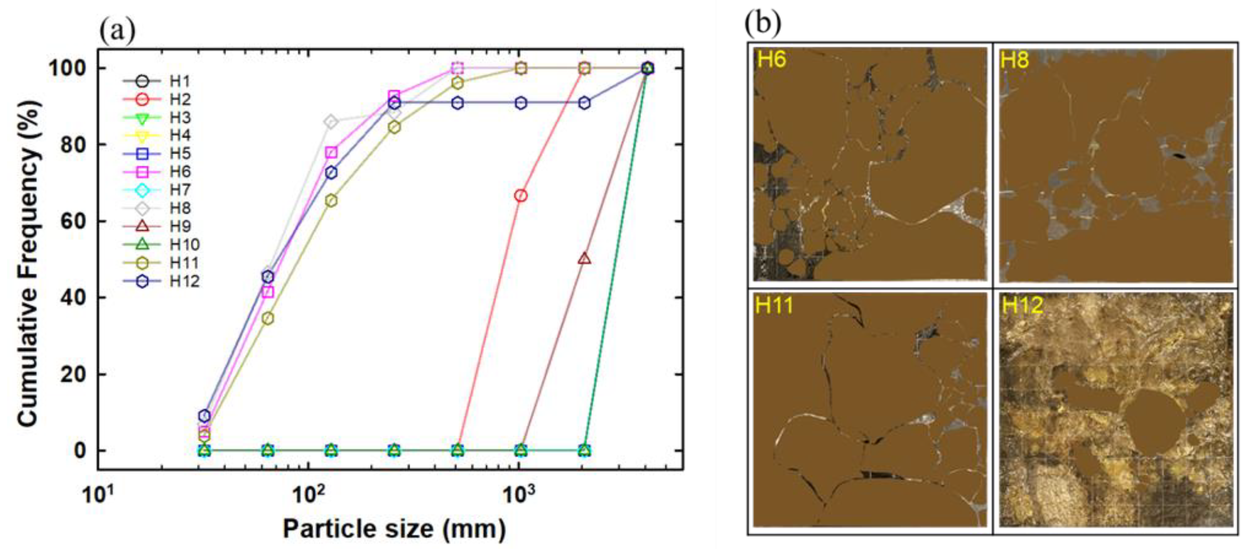
To investigate the physical characteristics of the field channel, the water depth, water temperature, flow velocity, and bed substrate were characterized.

Table 1. Physical factors, distance from a reference point (H1), temperature, flow velocity (u), water depth (h), and the median of the bed substrate sizes (D₅₀), of each surveyed, reach in the river.

Reach	H1	H2	H3	H4	H5	H6	H7	H8	H9	H10	H11	H12
Habitat type	step riffle	riffle	pool	riffle	riffle	pool	pool	pool	riffle	riffle	step riffle	pool
Distance (m)	0	4.6	8.3	10.1	14.9	19.6	33.1	36.8	39.5	44.5	51.8	58.2
Temperature (°C)	21.0	21.1	21.4	21.7	21.8	22.0	22.7	22.7	22.8	23	23.2	23.7
u (m s−1)	0.372	0.958	0.355	0.768	0.846	0.072	0.012	0.048	0.624	0.529	1.207	0.131
h (m)	0.272	0.263	0.734	0.074	0.082	0.727	0.920	0.789	0.387	0.308	0.290	0.868
D50 (mm)	>4096	896	>4096	>4096	>4096	79	> 4096	70	2048	>4096	96	75
Substrate	very large boulders	large boulders, medium boulders	very large boulders	very large boulders	very large boulders	very large boulders, medium boulders, small boulders, large cobbles	very large boulders	very large boulders, small boulders, large cobbles, small cobbles	very large boulders, large boulders	very large boulders	large boulders, medium boulders, small boulders, large cobbles	very large boulders, small boulders, large cobbles, small cobbles

provides the physical characteristic results. The field is connected to the valley. The pools had water depths between 0.73 and 0.92 m and flow velocities between 0.01 and 0.36 m s⁻¹. The riffles had water depths between 0.07 and 0.39 m and flow velocities between 0.53 and 0.96 m s⁻¹. As demonstrated in Figure 3, the pool reaches (H3, H6, H7, H8, and H12) were relatively deep, and the flow velocities were low. At the riffle reaches (H2, H4, H5, H9, and H10), the water was shallow, and the flow velocities were high. In addition, the step riffles had similar depths but differed in flow velocity. One (H1) had a lower flow velocity than the riffle reaches, while another (H11) had a higher flow velocity, indicating that the same habitat may not necessarily have the same tendency. All measurements were taken sequentially from H1 to H12 in the morning when the temperature was rising slowly. Therefore, the water temperature gradually increased from 21.0 °C to 23.7 °C (at H1 to H12). The field sites were in a mountain stream section connected to the valley, which exhibits the characteristics of a meandering channel with a large curvature. The bed substrates were constructed of a mix of very large boulders (4096–2048 mm), large boulders (2048–1024 mm), medium boulders (1024–512 mm), small boulders (512–256 mm), large cobbles (256–128 mm), and small cobbles (128–64 mm) as defined by the Wentworth scale (Wentworth, 1922). It was difficult to find gravels (2–16 mm), sands, or silts, as shown in Figure 2. The cumulative frequency curve (provided in Figure 4) indicates the percentile of the sediments in the reaches. The median point of the distribution (D₅₀) for each reach site was computed by the linear interpolation between the large and low particle sizes and is summarized in Table 1. Pool H3, H7, riffle H4, H5, and H10 and the step riffle H1 are composed of very large boulders. Therefore, they had D₅₀ over 4096 mm. The pool H6, H7, H12, and step riffle H11 had a D₅₀ below 100 mm.

3.2. Underwater Acoustic Characteristics by Habitat Type

The equivalent noise level (L_eq) compared the underwater environmental noise of the different habitats, and the results are provided in

Table 2. Equivalent noise level of the surveyed habitat types.

Habitat Type	Riffle					Pool					Step Riffle
Reach	H2	H4	H5	H9	H10	H3	H6	H7	H8	H12	H1	H11
Leq (dB)	152.25	155.06	154.30	135.71	142.45	141.72	139.69	109.13	108.94	111.25	148.92	145.29
Average (dB re 1 μPa)	147.95 ± 3.37					122.15 ± 1.16					147.11 ± 1.82

. The equivalent noise level was 147.95 dB re 1 μPa in the riffles and 122.15 dB re 1 μPa in the pools. It was 147.11 dB re 1 μPa in the step riffles, which is similar to the riffles level.

H2, H4, H5, H9, and H10 were characterized as riffles, and their sound distributions are provided in Figure 5. The sound pressure level of H2 decreased from a high value (146 dB re 1 μPa) at a low frequency, then increased again at 160 Hz, and decreased again at 1250 Hz. H5 generally exhibited lower SPLs than H2, but showed higher levels between 20 and 80 Hz, as well as over 4000 Hz. H4 had high SPLs of more than 140 dB re 1 μPa up to 16 Hz. The levels decreased up to 160 Hz, were maintained at 100 dB re 1 μPa or less up to 800 Hz, increased again up to 2500 Hz, and then decreased again from 110.9 dB re 1 μPa. H4 exhibited lower SPLs than H5 over all frequency bands. This appears to be due to shallower water depth and lower flow velocity than H5. H9, which exhibited a lower flow velocity than H4, had lower SPLs than H4. In H9, the levels reached 82.8 dB re 1 μPa at 160 Hz, increased again at 1000 Hz, and then decreased again. At over 1000 Hz, the level fluctuated between 89.2 dB re 1 μPa and 96.5 dB re 1 μPa. H10 had a lower flow velocity than H9 and exhibited lower SPLs than H9 between 12.5 and 31.5 Hz, but later showed higher SPLs than H9 and H4. This result was unlike the other SPLs that tended to decrease with the increasing flow velocity.

As shown in Figure 6 and Table 1, H3, H6, H7, H8, and H12 were pool-type habitats with low flow velocities and relatively deep waters. Figure 6 demonstrates the underwater acoustic characteristics of these sites. H3 and H6 exhibited high SPLs (over 129 dB re 1 μPa and 124 dB re 1 μPa) up to 31.5 and 40 Hz, respectively. The levels then sharply decreased and increased again at 100 and 250 Hz. They also exhibited characteristic peaks at 800 and 630 Hz. Thereafter, the levels decreased again with the higher band frequencies. H3 and H6 both had water depths of 0.73 m and flow velocities of 0.36 and 0.07 m s⁻¹, respectively. As for bed substrates, H3 was composed of very large boulders, while H6 consisted of a variety of very large, medium, and small boulders, and large cobbles. H7, H8, and H12 had water depths of 0.92, 0.79, and 0.87 m, respectively, and flow velocities of 0.01, 0.05, and 0.13 m s⁻¹, respectively, indicating similar hydraulic characteristics. In addition, in relation to bed substrates, H7 was composed of very large boulders, while H8 and H12 were composed of very large boulders, small boulders, large cobbles, and small cobbles. These three reaches exhibited very similar underwater acoustic characteristics for under 160 Hz and over 1000 Hz.

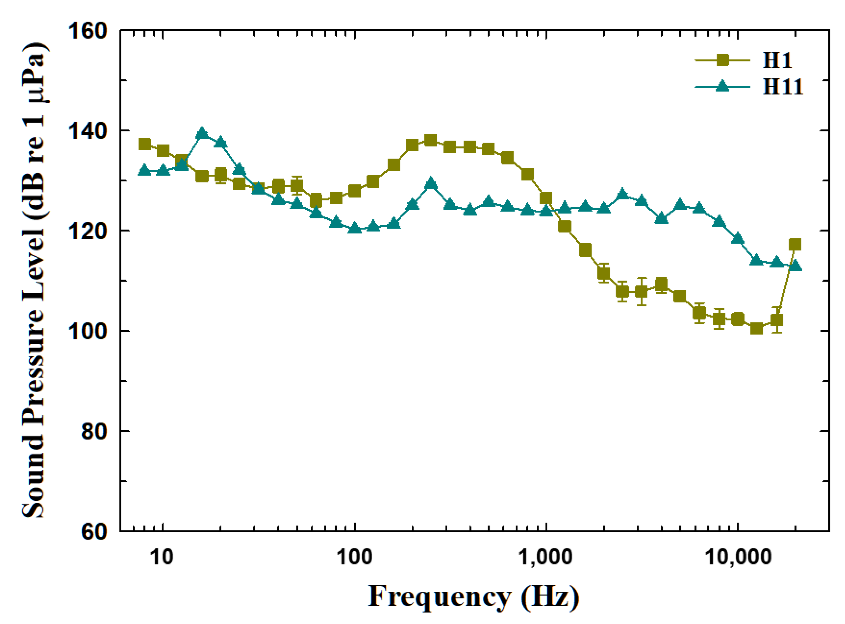
H1 and H11 were classified as step riffles. The water depths at the bottom of the steps were 0.27 and 0.29 m, respectively, and the flow velocities were 0.37 and 1.21 m s⁻¹, respectively. In relation to bed substrates, H1 was composed of very large boulders, and H11 consisted of large to small boulders and large cobbles. H1 had a bed structure with a very large, eroded boulder with an assemblage of several round boulders (Figure 2). The water current was strong, generating many water bubbles. The channel width remained consistent with the top of the step. H11 had very large boulders on both sides, and the channel width sharply narrowed, resulting in a very high flow velocity compared to the other reaches. As for the acoustic characteristics of these two reaches, high SPLs (over 120 dB re 1 μPa) were observed up to 1250 Hz, and the SPLs of H1 gradually decreased from 1250 to 12,500 Hz as demonstrated in Figure 7.

The habitat types of the field reaches were classified into riffles, pools, and step riffles. For each type, the SPLs with frequency signals were averaged and are illustrated in Figure 8. The average SPLs with the frequency signals are noticeably higher in the order of pools, riffles, and step riffles. Moreover, the SPLs (especially in the frequency range from approximately 63 Hz to 1600 Hz) had pronounced peak trends with habitat types.

On average, pools exhibited low SPLs, whereas riffles exhibited the characteristic peaks of high SPLs below 100 Hz. In pools, the lowest SPLs (between 84 dB and 89 dB re 1 μPa) were observed at 100 Hz and 160 Hz. Step riffles generally exhibited higher SPLs than pools and riffles and exhibited characteristic peaks between 100 and 1000 Hz.

Using these results, the slope β and the determination coefficient r² of the linear regression were established at each frequency (f) to determine the relationships between the SPLs measured in the riffles and pools with water depth and flow velocity (the two major hydraulic characteristics). The slope β and the r-squared(r²) represented positive or negative correlation and a measure of the quality of fit of a regression line. The slope β and the determination coefficients r² of the linear regression were calculated for the riffles (

Table 3. The slope β, regression intersect α, and the determination coefficient r² of the linear regression for the relationship between underwater SPL(Y) and flow velocity/water depth(X) in the riffle. n = 5 is the number of spots, including all riffles, and n = 4 is except to H10 from those.

Frequency (Hz)	Riffle
	Flow Velocity						Water Depth
	n = 4			n = 5			n = 4			n = 5
	β	α	r2	β	α	r2	β	α	r2	β	α	r2
8	0.528	100.080	0.443	0.325	117.400	0.325	−0.619	154.710	0.706	−0.582	154.560	0.691
10	0.775	75.771	0.862	0.431	105.140	0.524	−0.541	148.610	0.486	−0.502	148.450	0.469
12.5	0.668	84.628	0.860	0.591	91.179	0.891	−0.466	147.370	0.485	−0.563	147.760	0.535
16	0.477	98.225	0.641	0.587	88.784	0.818	−0.463	145.640	0.700	−0.616	146.260	0.595
20	0.544	87.296	0.838	0.550	86.846	0.912	−0.333	137.500	0.363	−0.458	138.000	0.419
25	0.619	78.731	0.728	0.606	79.831	0.835	−0.434	136.930	0.415	−0.559	137.430	0.470
31.5	0.508	85.827	0.604	0.531	83.909	0.766	−0.395	134.370	0.422	−0.512	134.840	0.472
40	0.571	79.584	0.461	0.504	85.308	0.563	−0.505	135.380	0.418	−0.575	135.660	0.485
50	0.575	78.769	0.430	0.468	87.950	0.484	−0.490	134.610	0.361	−0.539	134.810	0.424
63	0.615	73.145	0.633	0.408	90.849	0.519	−0.436	131.070	0.367	−0.443	131.100	0.404
80	0.877	43.949	0.819	0.455	79.954	0.437	−0.448	123.010	0.248	−0.403	122.840	0.227
100	1.070	23.012	0.882	0.481	73.290	0.350	−0.546	119.500	0.266	−0.447	119.110	0.200
125	1.133	15.505	0.898	0.465	72.503	0.291	−0.607	118.240	0.299	−0.473	117.700	0.199
160	1.153	12.617	0.935	0.469	71.039	0.296	−0.584	116.520	0.278	−0.449	115.970	0.179
200	1.177	11.551	0.940	0.547	65.310	0.401	−0.581	117.280	0.265	−0.485	116.890	0.208
250	1.198	11.129	0.882	0.821	45.313	0.737	−0.584	118.580	0.243	−0.645	118.820	0.301
315	1.312	1.367	0.931	0.828	42.663	0.694	−0.526	116.760	0.173	−0.564	116.910	0.213
400	1.316	0.859	0.970	0.896	36.742	0.795	−0.404	114.170	0.106	−0.495	114.540	0.161
500	1.278	4.424	0.965	0.764	48.269	0.662	−0.311	112.780	0.066	−0.346	112.920	0.090
630	1.201	12.108	0.924	0.707	54.316	0.618	−0.291	113.930	0.063	−0.317	114.040	0.082
800	1.004	30.577	0.835	0.607	64.475	0.586	−0.195	114.730	0.036	−0.232	114.880	0.057
1000	0.877	43.183	0.854	0.524	73.320	0.588	−0.133	115.970	0.023	−0.167	116.100	0.039
1250	1.074	27.745	0.945	0.546	72.823	0.484	−0.297	119.530	0.084	−0.265	119.400	0.075
1600	1.034	30.771	0.996	0.441	81.418	0.351	−0.385	121.130	0.160	−0.292	120.760	0.102
2000	1.089	24.953	0.986	0.550	71.014	0.498	−0.496	121.970	0.236	−0.438	121.740	0.209
2500	0.979	33.752	0.985	0.497	74.855	0.504	−0.446	120.920	0.237	−0.396	120.720	0.212
3150	0.875	41.647	0.991	0.444	78.390	0.507	−0.362	118.820	0.197	−0.322	118.660	0.176
4000	0.750	49.801	0.878	0.346	84.253	0.369	−0.438	118.500	0.346	−0.367	118.220	0.275
5000	0.617	59.757	0.621	0.269	89.501	0.231	−0.493	119.010	0.458	−0.410	118.680	0.355
6300	0.596	58.223	0.586	0.192	92.722	0.112	−0.574	117.430	0.627	−0.442	116.900	0.391
8000	0.490	64.128	0.410	0.110	96.639	0.036	−0.637	116.140	0.801	−0.480	115.510	0.457
10,000	0.383	71.252	0.296	0.036	100.810	0.004	−0.585	113.600	0.802	−0.423	112.950	0.397
12,500	0.254	79.057	0.163	−0.010	101.560	0.000	−0.470	108.800	0.645	−0.333	108.250	0.308
16,000	0.223	81.111	0.176	0.044	96.378	0.013	−0.366	106.320	0.549	−0.283	105.990	0.348
20,000	0.247	91.728	0.772	0.168	98.477	0.647	0.028	110.940	0.011	−0.002	111.060	0.000

) and pools (

Table 4. The slope β, regression intersect α, and the determination coefficient r² of the linear regression for the relationship between underwater SPL(Y) and flow velocity/water depth(X) in a pool. n = 5 is the number of spots, including all pools, and n = 4 is except to H8 from those.

Frequency (Hz)	Pool
	Flow Velocity						Water Depth
	n = 4			n = 5			n = 4			n = 5
	β	α	r2	β	α	r2	β	α	r2	β	α	r2
8	1.143	90.228	0.433	1.306	85.014	0.487	−2.676	323.930	0.991	−2.461	299.940	0.663
10	1.138	89.185	0.384	1.294	84.163	0.442	−2.835	335.720	0.994	−2.622	311.930	0.695
12.5	1.036	88.661	0.356	1.183	83.956	0.416	−2.685	321.500	0.996	−2.486	299.370	0.705
16	1.023	89.368	0.350	1.183	84.248	0.411	−2.675	321.260	0.998	−2.469	298.310	0.688
20	1.064	87.689	0.368	1.216	82.802	0.428	−2.703	322.440	0.990	−2.499	299.680	0.692
25	1.120	86.186	0.368	1.257	81.770	0.426	−2.834	332.360	0.984	−2.634	310.050	0.717
31.5	0.730	90.033	0.192	0.880	85.212	0.257	−2.534	306.260	0.967	−2.354	286.230	0.705
40	0.345	95.566	0.052	0.471	91.512	0.096	−2.160	275.900	0.855	−2.024	260.840	0.676
50	0.380	90.670	0.064	0.532	85.798	0.117	−2.181	273.260	0.872	−2.027	256.100	0.648
63	−0.147	98.972	0.026	−0.065	96.333	0.005	−0.993	177.550	0.500	−0.934	170.990	0.422
80	−0.331	99.794	0.180	−0.283	98.250	0.145	−0.551	139.830	0.209	−0.532	137.720	0.197
100	−0.023	87.922	0.001	0.085	84.476	0.010	−0.921	162.430	0.522	−0.840	153.340	0.370
125	−0.052	90.803	0.019	0.005	88.993	0.000	−0.365	119.690	0.399	−0.326	115.380	0.266
160	0.204	82.654	0.186	0.264	80.742	0.259	−0.717	143.820	0.956	−0.656	136.940	0.614
200	0.212	85.408	0.388	0.277	83.299	0.424	−0.497	128.800	0.893	−0.434	121.800	0.398
250	0.263	88.699	0.365	0.379	84.979	0.379	−0.300	116.820	0.199	−0.205	106.210	0.042
315	0.289	90.407	0.453	0.437	85.680	0.391	−0.507	135.690	0.580	−0.387	122.300	0.118
400	0.407	89.834	0.601	0.556	85.057	0.500	−0.692	151.840	0.726	−0.561	137.220	0.195
500	0.293	95.440	0.418	0.500	88.785	0.327	−0.684	155.140	0.952	−0.522	137.130	0.137
630	0.198	96.704	0.188	0.381	90.855	0.237	−0.698	156.210	0.970	−0.558	140.620	0.195
800	0.367	91.435	0.287	0.462	88.391	0.355	−1.057	182.530	0.992	−0.957	171.430	0.584
1000	0.344	88.288	0.464	0.412	86.108	0.504	−0.773	155.950	0.979	−0.696	147.420	0.552
1250	0.337	86.941	0.566	0.386	85.360	0.595	−0.657	145.130	0.898	−0.595	138.190	0.540
1600	0.192	89.890	0.390	0.215	89.156	0.447	−0.448	129.030	0.884	−0.415	125.320	0.637
2000	0.086	88.378	0.060	0.133	86.874	0.122	−0.460	126.980	0.707	−0.418	122.250	0.462
2500	0.142	86.497	0.147	0.165	85.749	0.198	−0.535	131.970	0.872	−0.503	128.430	0.703
3150	0.086	88.156	0.100	0.106	87.517	0.149	−0.390	121.080	0.860	−0.366	118.410	0.684
4000	0.114	86.238	0.258	0.123	85.866	0.311	−0.307	112.770	0.817	−0.288	110.660	0.653
5000	0.061	86.525	0.368	0.068	86.304	0.425	−0.125	97.538	0.652	−0.115	96.418	0.472
6300	0.009	87.108	0.048	0.013	86.978	0.095	−0.027	89.397	0.164	−0.023	88.998	0.108
8000	−0.008	88.095	0.074	−0.005	87.990	0.025	0.020	86.389	0.201	0.021	86.242	0.213
10,000	−0.011	88.825	0.057	−0.007	88.707	0.027	0.060	83.804	0.712	0.061	83.717	0.715
12,500	−0.021	90.281	0.129	−0.018	90.174	0.100	0.087	82.930	0.923	0.086	82.982	0.922
16,000	0.060	91.117	0.449	0.062	91.051	0.488	0.019	90.440	0.019	0.024	89.912	0.027
20,000	2.991	106.530	0.922	0.298	106.580	0.928	−0.265	132.290	0.301	−0.243	129.900	0.238

) at five locations (n = 5) and four locations after excluding H10 (a riffle habitat) or H8 (a pool habitat), because they may have been influenced by upstream underwater acoustic characteristics (of H9 and H7, respectively) (n = 4 in Table 3 and Table 4), representing a similar data patterns (in Figure 5 and Figure 6).

In the riffles, the underwater sound levels (measured as SPL) at all sites (n = 5) showed strong positive correlations (β > 0, 0.75 < r² < 1) with flow velocity in the frequency bands of 12.5 Hz ≤ f ≤ 31.5 Hz and 400 Hz. The SPLs at the sites (excluding H10) (n = 4) showed strong positive correlations (β > 0, 0.75 < r² < 1) with flow velocity in the frequency bands of 10 Hz, 12.5 Hz, 20 Hz, and 80 Hz ≤ f ≤ 4000 Hz. As for the relationship with water depth, the SPLs at all sites (n = 5) showed moderate negative correlations (β < 0, 0.5 < r² < 0.75) in the frequency bands of 8 Hz, 12.5 Hz, and 16 Hz. The SPLs measured at the sites excluding H10 (n = 4) showed strong negative correlations (β < 0, 0.75 < r² < 1) with water depth in the frequency band of 8000 Hz ≤ f ≤ 10,000 Hz and moderate negative correlations (β < 0, 0.5 < r² < 0.75) in the frequency bands of 8 Hz and 16 Hz.

In the pools, the SPLs had clearly defined positive correlations with flow velocity for both n = 5 and n = 4 (excluding H8), with moderate positive correlations (β > 0, 0.5 < r2 < 0.75) in the frequency bands of 400 Hz and 1250 Hz. Between SPL and water depth, very strong negative correlations (β < 0, 0.75 < r2 < 1) were observed in the frequency bands of 12,500 Hz, and moderate negative correlations (β < 0, 0.5 < r² < 0.75) were noted in f ≤ 50 Hz, 160 Hz, 800 Hz ≤ f ≤ 1600 Hz, 2500 Hz ≤ f ≤ 4000 Hz, and 10,000 Hz for n = 5. For n = 4, very strong negative correlations (β < 0, 0.75 < r² < 1) were noted in the frequency bands of f ≤ 50 Hz, 160 Hz ≤ f ≤ 200 Hz, 500 Hz ≤ f ≤ 1600 Hz, 2500 Hz ≤ f ≤ 4000 Hz, and 12,500 Hz. Moderate negative relations (β < 0, 0.5 < r² < 0.75) were observed in the bands 63 Hz, 100 Hz, 315 Hz ≤ f ≤ 400 Hz, 2000 Hz, 5000 Hz and 10,000 Hz at the sites, excluding H8.

4. Discussion

Sounds in a channel can be sub-categorized as emanating from the abiotic and biotic factors of the channel [15]. The abiotic factors include sounds caused by water flow, collisions with bed substrates, and those transmitted from the atmosphere to the water. The biotic factors include sounds caused by the movement or phonation of aquatic life forms and sounds emitted by living organisms in the atmosphere. Considering these factors, the underwater acoustic characteristics of different habitat types were analyzed. The field reaches were connected in the valley of the Namdae Stream. The water depth was generally shallow, and the water was fairly transparent; Melanian snails were visible in the field area. While fish were occasionally observed in pools downstream of the study area, living organisms, such as fish, were almost absent in the reach sites. According to River Namdae Yangyang Master Plan Report [24], it was reported that Zacco koreanus and Zacco platypus were inhabited downstream by field investigations but upstream was not almost observed because the artificial weirs located downstream disturbed fish migration or installing appropriate fishways. Therefore, most of the acoustics could only be created by abiotic factors. Consequently, the underwater sounds were probably caused by the abiotic factors of flow velocity, bed substrate, and water depth. Variations in the sound-propagation environment can be affected by sound speed variations as determined by temperature, density, salinity [25] and the medium through which sound waves propagate. For example, the speed of sound is approximately 1481 m/s in water at a temperature of 20 ℃. In contrast, in air at the same temperature, the speed of sound is 343 m/s (propagation velocities, along with the density of the material). Freshwater rivers have low salinity compared to seawater, with the density varying with water temperature. The temperature in each of the reaches varied by less than 2.7 °C (Table 1), with density differences ranging within 0.001 g/cm³. Hence, the water density-derived sound speed variations were considered to be negligible.

Fish experts suggest 140 dB re 1 μPa as the criteria for fish damage, and the sound pressure causes the fish to move into deeper areas or demonstrate escape responses because they are surprised and perceive a threat [26]. An underwater noise of 140 dB re 1 μPa or less is the mandatory level in domestic damage assessment criteria of cultured fish due to the noise and vibrations [27]. The riffles and step riffles of the Namdae Stream exhibited underwater background sounds exceeding this criterion. Fish were not observed in the riffles and step riffles. Thus, fish did not influence the underwater sound measurements. The equivalent noise level (L_eq) is the average value of the continuous SPLs of various frequency bands and is mainly used to assess environmental noise. The L_eq is 100 dB or less in habitats with no flow and 110 dB or more in habitats with fast flow [13]. According to Tougaard et al. [28], which reviewed and compared available measurements of underwater noise during the operation of wind turbines and ship noise, the total sound pressure level (L_eq) over 30 s segments of the sound recordings was reported in a range of 81 dB ~ 137 dB re 1μPa. In this study, high equivalent noise levels occurred in pools with a slow flow. This may be due to the transfer of underwater sounds caused by the surrounding reaches and ambient noises.

Riffles are created by rapidly changing bed slopes. Due to the high flow velocity, riffles have sharply changing terrain and bed structures [29]. Pools are deep bodies of water with relatively deep water and almost no flow velocity and are created by erosion and accumulation caused by a high-flow velocity upstream. Step riffles are vertically developed with sharp bed slopes and heads at narrow channel sections when compared to riffles and pools, which are created by gentle bed slopes at wide channel sections [30].

As shown in Table 1 and Figure 5, among the riffle sites, H2 and H5 had relatively faster flow velocities and possessed high spectral SPLs with frequencies below 5000 Hz.

As presented in Table 3, the SPL in riffles was significantly affected by the flow velocity. Furthermore, underwater sounds were also influenced by bed substrates. The bed substrates of these sites were mostly very large, large, and small boulders, indicating that the sounds could be created by friction between the water flow and bed substrates. The acoustics in the water is influenced by the pressure of water from upstream.

In the low-frequency bands of the pools, H3 and H6 exhibited high SPLs, while H7, H8, and H12 exhibited low SPLs. As they exhibited different underwater acoustic characteristics despite having the same habitat types, additional factors must be considered. The underwater environment is formed by various physical factors, such as the roughness of the bed substrates, channel width, and flow characteristics, which can all influence underwater acoustic characteristics [11].

H3 and H6 were pools that exhibited very similar acoustic characteristics with similar underwater sounds caused by similar water depths and the influence of the upstream riffle of H2 and H5, respectively. As sounds in the low-frequency bands generated by a riffle can be readily propagated through the deep water of a pool, the high SPLs at 60 Hz or less may be transmitted from H2 and H5. In addition, upstream sounds are expected to be transmitted in the frequency band between 600 and 800 Hz, and thus, high SPLs were observed even though they were at lower levels than the low-frequency bands. The low-frequency bands of underwater sounds have limited influence on organisms living in rivers or streams because they have longer wavelengths than those in shallow waters. Therefore, only a very small proportion is transmitted [31]. Low-frequency sounds thus attenuate more quickly as they travel in shallow water relative to deep water and can be transmitted further in deeper water. In boulder beds, the lowest frequency that can travel in 1 m-deep water is approximately 300 Hz, whereas, in 10 m-deep water, the lowest frequency is approximately 30 Hz [16]. For this reason, low-frequency SPLs were high in pools with low flow velocities. Low-frequency propagation is strongly affected by depth. Therefore, fish in shallow habitats can detect lower-frequency sounds [16]. The H10 results support these findings, as the bed substrate of H10 was very rough in large boulders due to the high-water flow. The roughness was not calculated, but we observed small boulders combined with very large ones, appearing similar to a hump (Figure 2).

The pools, H7, H8, and H12, had similar hydraulic characteristics and underwater acoustic characteristics. The natural underwater acoustic characteristics of pools were comparable because they had similar physical environments, and the sound frequencies transmitted from upstream were minimized. Characteristic peaks commonly occurred at 80 and 125 Hz, and the SPL decreased in the order of H12, H7, and H8 between 125 and 1000 Hz. This order reflects the higher flow velocity at H12 when compared to the other two sites. H7 had higher SPLs than H8 because it was affected by the upstream sounds.

In the step riffles, the sounds at the head of the step were mostly generated by the accumulation of boulders and the resulting scour of the bottom substrate and were affected more by the horizontal space and height of the step than by the bed slope [32]. Therefore, the sounds created by the head of the step were closely related to the boulders that constitute the step.

We believe that a head with high energy existed at H11 because of the high flow velocity. Less energy was caused by the head in the larger channel with an embossed bed structure (H1), which resulted in reduced underwater SPLs in the high-frequency bands when compared to those of H11.

Step structures cause a head due to the high bed slope and accumulation of boulders in a narrow channel width and, therefore, develop vertically when compared to a riffle-pool bed structure [19,27,29]. In vertically developed step riffles, turbulent flows are generated by the tumbling flows and jet-and-wake flows [29]. A large volume of water splash was generated at H1, with its high bed roughness. Therefore, H1 incorporated a diverse array of tumbling and turbulent flows. For this reason, H1 exhibited higher SPLs than H11 (between 30 and 1000 Hz), even though its flow velocity was lower than that of H11. Over 1000 Hz, the underwater sounds in H11 appeared to reflect the higher head energy, which generated higher SPLs than at H1.

The SPLs of underwater sounds were averaged for each channel type, and the average SPLs were found to be higher in the order of step riffles > riffles > pools. The acoustic characteristics (as a function of habitat type) were analyzed through site investigations. The differences in the hydromorphology of each habitat type had different acoustic characteristics. Wysocki et al. [13] reported the characteristic peaks with their main energy in low-frequency bands to occur in static areas, such as lakes and ponds, and a sharp energy decrease occurs with frequency bands between 100 and 800 Hz. Wysocki et al. [13] also noted that the energy at frequency bands between 200 Hz and 5 kHz was much higher in areas with water flow, such as rivers and streams than in static areas. This study supports these findings, pools with low flow velocity mainly possessed low acoustic energy, while riffles or step riffles with high flow velocity had high acoustic energy.

The linear regression determined the correlations between the SPLs measured in the riffles and pools and flow velocity/water depth. Very strong positive correlations were identified between SPL and flow velocity in the frequency band of 63 Hz ≤ f ≤ 6300 Hz in the riffles when H10 was excluded. In the pools (except for H8), very strong negative correlations were observed in the frequency bands of f ≤ 50 Hz and 315 Hz ≤ f ≤ 5000 Hz. The underwater sound levels were very closely associated with hydraulic habitat characteristics, such as flow velocity and water depth, depending on habitat types. This implies that the underwater sound level (measured as SPL) can be used to estimate flow velocity and water depth in aquatic habitats. However, it is not suggested as practical to extrapolate this result for use outside of this data set.

Prime habitats for aquatic organisms are limited and significantly depend on the various physical characteristics of the channels. Efforts are being made to preserve or restore biological habitats through projects such as the ecological restoration of channels. Therefore, methods for assessing habitats suitable for living organisms are being actively discussed and experimented with.

5. Conclusions

This study investigated the relationship between underwater acoustic characteristics and the hydraulic characteristics of habitats to assess biological habitats. To analyze underwater acoustic characteristics by fluvial habitat type, the stream reaches of the Namdae Stream in Yangyang, South Korea, were classified into riffles, pools, and step riffles using their hydraulic characteristics, and their underwater acoustic characteristics were assessed. A total of 12 reaches in the upstream section were analyzed, and their habitat types were classified. Their hydraulic characteristics, such as the flow velocity, water depth, and bed substrate, were compared with their underwater acoustic characteristics. In conclusion, various characteristics were consistent with habitat type and hydraulic conditions, based on a specific underwater acoustic measurement methodology which is proposed as a new method to assess biological habitats instead of other classical measures. The results indicate that underwater acoustic sounds are significantly affected by the acoustic characteristics of the adjacent upstream reach, as well as the flow velocity, water depth, and bed substrate roughness. Underwater sounds exhibit specific characteristics according to habitat types and hydraulic conditions.

References

- Arthington, A.H.; Bunn, S.E.; Poff, N.L.; Naiman, R.J. The challenges of providing environmental flow rules to sustain river ecosystems. Ecol. Appl. 2006, 16, 1311–1318. [Google Scholar] [CrossRef] [Green Version]
- Hur, J.W.; Park, Y.; Kang, S.U.; Kim, J. Physical habitat assessment of pale chub (Zacco platypus) to stream orders in the Geum River basin, Korea. J. Environ. Biol. 2009, 27, 397–405. [Google Scholar]
- Kim, H.J.; Kim, C.W.; Woo, H.S. Effects and alternatives of transversal structures on the ecological development of rivers. Spec. Issue Eco Friendly Constr. 2003, 51, 42–58. [Google Scholar]
- Lee, G.-S.; Lee, H.-S. Evaluation of possibility for the classification of river habitat using imagery information. J. Korean Assoc. Geogr. Inf. Stud. 2012, 15, 91–102. [Google Scholar] [CrossRef] [Green Version]
- Gorman, O.T.; Karr, J.R. Habitat structure and stream fish communities. Ecology 1978, 59, 507–515. [Google Scholar] [CrossRef]
- Angermeier, P.L.; Karr, J.R. Fish communities along environmental gradients in a system of tropical streams. Environ. Biol. Fishes 1983, 9, 117–135. [Google Scholar] [CrossRef]
- Poff, N.L.; Allan, J.D. Functional organization of stream fish assemblages in relation to hydrological variability. Ecology 1995, 76, 606–627. [Google Scholar] [CrossRef]
- Rowe, D.C.; Pierce, C.L.; Wilton, T.F. Fish assemblage relationships with physical habitat in wadeable Iowa streams. North Am. J. Fish. Manag. 2009, 29, 1314–1332. [Google Scholar] [CrossRef] [Green Version]
- Tonolla, D.; Lorang, M.S.; Heutschi, K.; Tockner, K. A flume experiment to examine underwater sound generation by flowing water. Aquat. Sci. 2009, 71, 449–462. [Google Scholar] [CrossRef] [Green Version]
- Tonolla, D.; Acuna, V.; Lorang, M.S.; Heutschi, K.; Tockner, K. A field-based investigation to examine underwater soundscapes of five common river habitats. Hydrol. Process. 2010, 24, 3146–3156. [Google Scholar] [CrossRef]
- Amoser, S.; Ladich, F. Year-round variability of ambient noise in temperate freshwater habitats and its implications for fishes. Aquat. Sci. 2011, 72, 371–378. [Google Scholar] [CrossRef] [PubMed] [Green Version]
- Hawkins, A.D.; Myrberg, A.A. Hearing and sound communication under water. In Bioacoustics, A Comparative Approach; Lewis, B., Ed.; Academic Press: London, UK, 1983; pp. 347–405. [Google Scholar]
- Wysocki, L.E.; Amoser, S.; Ladich, F. Diversity in ambient noise in European freshwater habitats: Noise levels, spectral profiles, and impact on fishes. J. Acoust. Soc. Am. 2007, 121, 2559–2566. [Google Scholar] [CrossRef] [PubMed]
- Ladich, F. Sound Communication in Fishes (Animal Signals and Communication); Springer-Verlag: Berlin, Germany, 2015. [Google Scholar]
- Amoser, S.; Ladich, F. Are hearing sensitivities of freshwater fish adapted to the ambient noise in their habitats? J. Exp. Biol. 2005, 208, 3533–3542. [Google Scholar] [CrossRef] [Green Version]
- Popper, A.N.; Carlson, T.J. Application of sound and other stimuli to control fish behavior. Trans. Am. Fish. Soc. 1998, 127, 673–707. [Google Scholar] [CrossRef]
- Kim, W.-K.; Lee, C.-S.; Lee, Y.-Y.; Baik, K.-K.; Hur, S.-B. Environmental factors and population density of brackish water clam, Corbicula Japonica on Namdae Stream in Yangyang, Gangwon. J. Aquac. 2002, 15, 1–6. [Google Scholar]
- Kim, C.-H.; Lee, W.-O.; Hong, K.-E.; Lee, C.-H.; Kim, J.-H. Ichthyofauna and fish community structure in Namdae Stream, Yangyang, Korea. Korean J. Ichthyol. 2006, 18, 112–118. [Google Scholar]
- Ministry of Environment (MOE). Water Environment Information System (WEIS). 2017. Available online: https://water.nier.go.kr (accessed on 5 March 2021).
- Korea Meteorological Administration (KMA). Available online: https://data.kma.go.kr (accessed on 10 March 2021).
- Wentworth, C.K. A scale of grade and class terms for clastic sediments. J. Geol. 1922, 30, 377–392. [Google Scholar] [CrossRef]
- Lurton, X. An Introduction to Underwater Acoustics, Principles and Applications, 2nd ed.; Springer: New York, NY, USA, 2010. [Google Scholar]
- Blevins, R.D. Formulas for Dynamic, Acoustics and Vibration; John Wiley & Sons: Chichester, UK, 2015; pp. 134–202. [Google Scholar] [CrossRef]
- Ministry of Land (MOL). River Namdae Yangyang Master Plan Report. 2011. Available online: https://me.go.kr (accessed on 2 April 2022).
- Nedelec, S.L.; Campbell, J.; Radford, A.N.; Simpson, S.D.; Merchant, N.D. Particle motion: The missing link in underwater acoustic ecology. Methods Ecol. Evol. 2016, 7, 836–842. [Google Scholar] [CrossRef] [Green Version]
- Choi, T.H.; Kim, J.H.; Song, H.L.; Ko, C.S. Suggestion of safety level in fish farming by impulsive sound. Tunn. Undergr. Space 2015, 25, 125–132. [Google Scholar] [CrossRef] [Green Version]
- Ministry of Environment (MOE). National Environmental Dispute Resolution Commission. 2009. Available online: http://ecc.me.go.kr (accessed on 15 March 2021).
- Tougaard, J.; Hermannsen, L.; Madsen, P.T. How loud is the underwater noise from operating offshore wind turbines? J. Acoust. Soc. Am. 2020, 148, 2885–2893. [Google Scholar] [CrossRef]
- Lee, D.-J.; Byeon, H.-K.; Chio, J.-K. Characteristics of fish community in gap stream by habitat type. Korean J. Limnol. 2009, 42, 340–349. [Google Scholar]
- Montgomery, D.R.; Buffington, J.M. Channel reach morphology in mountain drainage basins. Geol. Soc. Am. Bull. 1997, 109, 596–611. [Google Scholar] [CrossRef]
- Rogers, P.H.; Cox, M. Underwater sound as a biological stimulus. In Sensory Biology of Aquatic Animals; Atema, J., Fay, R.R., Popper, A.N., Tavolga, W.N., Eds.; Springer: New York, NY, USA, 1988; pp. 131–149. [Google Scholar]
- Kim, S.W.; Chun, K.W.; Park, C.M.; Nam, S.Y.; Lim, Y.H.; Kim, S.Y. The morphologic characteristics of step-pool structures in a steep mountain stream, Chuncheon, Gangwon-do. J. Korean For. Soc. 2011, 100, 202–211. [Google Scholar]
Figure 1.
Location of the 12 field reaches in the Namdae Stream, Yangyang, South Korea, using a Drone (INSPIRE 1).
Figure 2.
Substrates of the 12 field reaches were placed under-sampling frame 1 by 1 m with a 10 × 10 cm grid.
Figure 3.
Mean (±S.D.) flow velocity and water depth of different reaches (H1–H12).
Figure 4.
Cumulative grain-size frequency curves (a) with indicated percentile values and shading of bed materials (b) to compute the size of the sediment.
Figure 5.
Sound pressure level versus ⅓ octave band frequency in riffles. The error bars illustrate the standard deviation of the obtained average.
Figure 6.
Sound pressure level versus ⅓ octave band frequency in pools. The error bars illustrate the standard deviation of the obtained average.
Figure 7.
Sound pressure level versus ⅓ octave band frequency in step riffles. The error bars illustrate the standard deviation of the obtained average.
Figure 8.
Sound pressure level versus ⅓ octave band frequency in three channel types. The error bars illustrate the standard deviation of the obtained average.