Conjunctive Water Management under Multiple Uncertainties: A Case Study of the Amu Darya River Basin, Central Asia

Abstract

With population growth, climate volatility, and economic expansion, the conjunctive management of surface–groundwater (SGW) faces great challenges. In this study, a hybrid factorial optimization programming (HFOP) method is developed through integrating factorial analysis, interval linear programming, flexible fuzzy programming, and two-stage stochastic programming into a general framework. HFOP can effectively reflect the multiple uncertainties and quantitatively identify the effects of multiple factors. Then, a HFOP-SGW model is formulated for the middle reaches of the Amu Darya River Basin, where 125 scenarios are analyzed. Some of the major findings are: (i) the improvement of surface-water transport efficiency and the proper use of groundwater can effectively alleviate regional water shortage; (ii) agricultural users have a high risk of water scarcity for all states, especially under a low-flow level; (iii) uncertainties of water-flow levels and risk-reverse attitudes of decision makers have significant impacts on the system’s benefits and water-allocation scheme; and (iv) the surface-water-transmission loss rate and risk perceptions of decision makers are the main factors affecting the system’s benefit’s and water-allocation scheme. These findings can help decision makers obtain desired water-allocation strategies to respond to the variations in water availability.

1. Introduction

The water-scarcity problem is a key factor restricting social and economic development. According to the United Nations World Water Development Report (2019), compared with 2015, the global water demand in 2050 will increase by 55%, and nearly 50% of the world’s population will face water shortage problems [1]. Severe regional water shortage problems have a serious impact on eco-environment, food security, human health, and economic development [2]. In particular, in Central Asia, the rapid expansion of agriculture caused more than 80% of the runoff to flow into farmland, leading the inflow from the Aral Sea decrease from 64.2 km³/a to 10.2 km³/a between 1960 to 2015 [3,4]. The shrinking of the Aral Sea caused a series of ecological problems, such as land salinization, biodiversity reduction, and the destruction of cultivated land [5]. The current single water-resource-allocation method causes a lot of waste of water resources, aggravates regional water-resource conflicts, and seriously restricts the healthy development of the region. The efficient coordinated management of surface and groundwater systems is urgently needed.

In recent decades, some optimization methods have been proposed for finding operating strategies in the surface–groundwater (SGW) system [6,7]. For example. Sepahvand et al. (2019) proposed a multi-objective optimization model based on the genetic programming method for achieving the optimal allocation patterns of surface water and groundwater [8]. Abbas A et al. (2020) proposed a cyclic storage system for a reliability-based optimum design of surface water and groundwater, based on the particle swarm optimization algorithm and linear programming method [9]. Qiao et al. (2021) developed an ecological stability-oriented double-layer model based on the large-scale system coordination method for optimizing the water-use structure in the Heihe River Basin, where a contradiction between agricultural water and ecological water obviously existed [10]. The above-mentioned research is effective in generating reasonable water-resource allocation strategies. However, the complexity and uncertainty of water-resource systems pose a major challenge for maintaining the stability of the SGW system. For example, the amount of water availability, which has random characteristics, is affected by natural processes (e.g., precipitation, evaporation, and climate change). The economic parameters are affected by social development and policy change, which present fuzzy nature. These inherent uncertainties would increase the difficulty of SGW system management and strongly influence the managers’ decision-making processes. More robust optimization methods are desired to tackle the uncertainties that exist in the SGW system.

Among the programming methods, two-stage stochastic programming (TSP), as a powerful optimization method, is effective for solving the uncertainty problems with known probabilities [11]. In addition, TSP can effectively balance the system’s benefits through introducing a recourse mechanism to ensure the robustness of the system [12,13]. Such a robust analytical approach can provide a comprehensive strategy for addressing regional water scarcity risks, especially in arid and semi-arid areas (i.e., Central Asia). In addition, SGW management may be affected by regional water-allocation rules and market policies (e.g., water-consumption restrictions and ecological protection mechanisms); the uncertainty of price parameters and engineering parameters are high, due to the lack of human subjective understanding and the complexity of water-resource systems [14]. The uncertainty of these issues is beyond the capabilities of TSP. Interval parameter programming (IPP) can handle uncertainty that can handle unknown deterministic probability distributions, expressed as interval parameters [15]; flexible fuzzy programming (FFP) can deal with a class of ambiguity problems caused by the limitations of the human cognitive level and social development, which exist in relaxed constraints [16]. Additionally, the complex correlations and interactions among the parameters exist in the SGW system and these complexities can significantly affect the system’s stability. Fortunately, factorial analysis is a useful method that can precisely obtain the full characteristic of the model parameter with less experimental design. Moreover, factorial analysis has a strong ability to reveal the main effects and potential interactions of the model’s parameters.

Therefore, in the present study, a hybrid factorial optimization programming (HFOP) method is developed through integrating factorial analysis technology, interval parameter programming (IPP), flexible fuzzy programming (FFP), and two-stage stochastic programming (TSP) into a general framework. An ensemble approach can significantly improve the trial performance of the HFOP in surface-water and groundwater management under multiple uncertainties. The innovations of this article can be summarized as follows: (i) HFOP can effectively tackle the uncertainties expressed as fuzzy sets, discrete intervals and probability distributions; (ii) HFOP can quantitatively identify the impact of the parameter’s main effects and interaction effects on the system’s benefits; and (iii) HFOP is applied to the SGW system for alleviating the contradiction between water supply and demand. The results obtained from the model hopefully generate desirable alternatives for the basin.

2. Methodology

2.1. General Framework of the HFOP

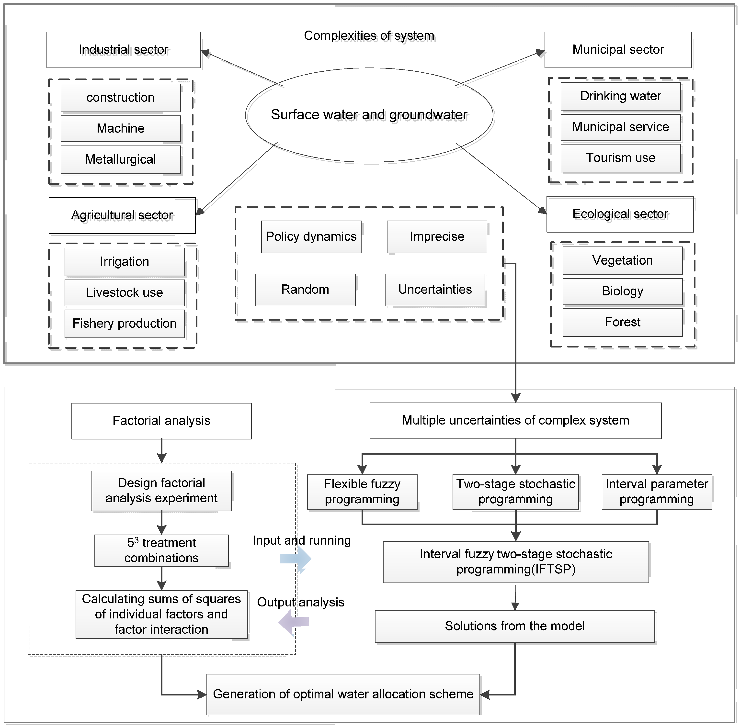
Obtaining the optimal water-resource allocation scheme in adaptation to climate change and water-shortage problems includes two components: uncertainty parameter processing and optimal scheme selection. The HFOP covers the two parts through integrating interval fuzzy two-stage stochastic programming (IFTSP) and factorial analysis into a general framework (as shown in Figure 1). Each subcomponent can enhance the capacity of HFOP in addressing the complex water-management problem. In detail, the interval fuzzy two-stage stochastic programming (IFTSP) can deal with uncertain problems in the optimal allocation of water resources, such as the volatility of the water-resource level, decision-making cognitive biases, and policy changes. Factorial analysis (FA) can effectively identify the interaction between factors and quantitatively characterize the contribution rate of the main factors. In general, HFOP can help decision makers identify the main factors in the water-resource system and obtain the optimal water-resource-allocation scheme.

2.2. Interval Fuzzy Two-Stage Stochastic Programming

The water-resources system is a complex and interrelated subject with multiple complexities and uncertainties (such as the uncertainty of policy information, fluctuations in market prices, climate change, and changes in water demand). Two-stage stochastic programming (TSP) is effective for handling these problems where an analysis of the policy scenario is desired and when the right-hand-side variables are random [17]. In TSP, the first-stage decision would be made before certain information is obtained; the second-stage decision is obtained by minimizing the “penalties” that may appear when the demand is not satisfied. A general TSP model can be formulated as follows:

$$Maxf={\displaystyle \sum _i^{I}N{b}_i}W{h}_i-E\left[{\displaystyle \sum _i^{I}P{e}_{i}W{l}_{iQ}}\right]$$

(1)

subject to:

$${\displaystyle \sum _{i=1}^m{A}_i(W{h}_i-W{l}_{iQ})}\le B_{j}i=1,2,\dots ,m;j=1,2,\dots ,g$$

(2)

$${\displaystyle \sum _{i=m+1}^I{A}_i(W{h}_i-W{l}_{iQ})}\le B_{j}i=m+1,m+2,\dots ,I;j=g+1,g+2,\dots ,n$$

(3)

$$W{h}_i\ge 0,W{l}_{iQ}\ge 0$$

(4)

where $W{h}_i$ is the first-stage decision variable when enough of certain information is not obtained; $N{b}_{i}W{h}_i$ is the net benefit of the first stage; $W{l}_{iQ}$ is the two-stage decision variable at each water flow (Q), which is the recourse for the event’s occurrence; $E\left[{\displaystyle \sum _i^{I}P{e}_{i}W{l}_{iQ}}\right]$ is the penalty for the second-stage decision; $N{b}_i$ is the coefficient of the first stage; $P{e}_i$ is the coefficient of the second-stage decision; and $A_i$ and $B_i$ are the coefficients of the constrains. The distribution of Q could be approximated by a discrete distribution, allowing Q take the discrete values of Q_r with probability levels of P_r (r = 1, 2, …, R, and ${\displaystyle \sum P_r=1}$). Thus we have $E\left[{\displaystyle \sum _i^{I}P{e}_{i}W{l}_{iQ}}\right]={\displaystyle \sum _i^I{\displaystyle \sum _r^R{P}_r}}P{e}_{i}W{l}_{ir}$. TSP model can efficiently deal with the problem with a known probability distribution. However, more parameters are presented as interval numbers due to the lack of useful information. Thus, through integrating the interval parameter programming into the TSP [18], the following interval two-stage stochastic programming (ITSP) can be formulated as:

$$Max{f}^{\pm }={\displaystyle \sum _i^{I}N{b}_i^{\pm }}W{h}_i^{\pm }-{\displaystyle \sum _i^I{\displaystyle \sum _r^R{P}_r^{\pm }}}P{e}_i^{\pm }W{l}_{ir}^{\pm }$$

(5)

subject to:

$${\displaystyle \sum _{i=1}^m{A}_i^{\pm }(W{h}_i^{\pm }-W{l}_{ir}^{\pm })}\le B_j^{\pm }i=1,2,\dots ,m;j=1,2,\dots ,g$$

(6)

$${\displaystyle \sum _{i=m+1}^I{A}_i^{\pm }(W{h}_i^{\pm }-W{l}_{ir}^{\pm })}\le B_j^{\pm }i=m+1,m+2,\dots ,I;j=g+1,g+2,\dots ,n$$

(7)

$$W{h}_i^{\pm }\ge 0,W{l}_{ir}^{\pm }\ge 0$$

(8)

Generally, although the ITSP approach is effective for handling the uncertainties expressed as interval and random, it cannot reflect the ambiguity and vagueness of the constraints due to the subjective experience and insufficient data. Flexible fuzzy programming (FFP) can be introduced into ITSP to tackle the above-mentioned uncertain problem [16]. Thus, an interval fuzzy two-stage stochastic programming (IFTSP) model is formulated as follows:

$$Max{f}^{\pm }={\displaystyle \sum _i^{I}N{b}_i^{\pm }}W{h}_i^{\pm }-{\displaystyle \sum _i^I{\displaystyle \sum _r^R{P}_r^{\pm }}}P{e}_i^{\pm }W{l}_{ir}^{\pm }$$

(9)

subject to:

$${\displaystyle \sum _{i=1}^m{A}_i^{\pm }(W{h}_i^{\pm }-W{l}_{ir}^{\pm })}\le B_j^{\pm }+(\tilde{\tau }(1-\gamma ))i=1,2,\dots ,m;j=1,2,\dots ,g$$

(10)

$${\displaystyle \sum _{i=m+1}^I{A}_i^{\pm }(W{h}_i^{\pm }-W{l}_{ir}^{\pm })}\le B_j^{\pm }i=m+1,m+2,\dots ,I;j=g+1,g+2,\dots ,n$$

(11)

$$W{h}_i^{\pm }\ge 0,W{l}_{ir}^{\pm }\ge 0$$

(12)

$$0\le \gamma \le 1$$

(13)

where $\gamma$ is a satisfaction level of flexible constraints, which should be given by the regional decision maker. $\tilde{\tau }$ is a triangular fuzzy number, which can be presented by its three prominent points (i.e., $\tilde{\tau }$ = (${\tau }_{\left(1\right)}$, ${\tau }_{\left(2\right)}$, ${\tau }_{\left(3\right)}$)) with a membership function of:

$$f_A(\tau )=\{\begin{array}{ll}\frac{\tau -{\tau }_{(1)}}{{\tau }_{(2)}-{\tau }_{(1)}}=f_A^L(\tau ),& {\tau }_{(1)}\le \tau \le {\tau }_{(2)}\\ \frac{{\tau }_{(3)}-\tau }{{\tau }_{(3)}-{\tau }_{(2)}}=f_A^R(\tau ),& {\tau }_{(2)}\le \tau \le {\tau }_{(3)}\\ 0& otherwise\end{array}$$

(14)

The fuzzy ranking can be obtained by the method [19], $\tilde{\tau }$ can be defuzzied as

$$\begin{array}{l}{\Re }_A=\frac{{\int }_{{\tau }_{(1)}}^{{\tau }_{(2)}}\tau f_A^L(\tau )d\tau +{\int }_{{\tau }_{(2)}}^{{\tau }_{(3)}}\tau f_A^R(\tau )d\tau }{{\int }_{{\tau }_{(1)}}^{{\tau }_{(2)}}{f}_A^L(\tau )d\tau +{\int }_{{\tau }_{(2)}}^{{\tau }_{(3)}}{f}_A^R(\tau )d\tau }\\ =\frac{{\int }_{{\tau }_{(1)}}^{{\tau }_{(2)}}\tau \frac{\tau -{\tau }_{(1)}}{{\vartheta }_{\tau }}d\tau +{\int }_{{\tau }_{(2)}}^{{\tau }_{(3)}}\tau \frac{{\tau }_{(3)}-\tau }{{\vartheta }_{\tau }^{\prime }}d\tau }{{\int }_{{\tau }_{(1)}}^{{\tau }_{(2)}}\frac{\tau -{\tau }_{(1)}}{{\vartheta }_{\tau }}d\tau +{\int }_{{\tau }_{(2)}}^{{\tau }_{(3)}}\frac{{\tau }_{(3)}-\tau }{{\vartheta }_{\tau }^{\prime }}d\tau }={\tau }_{(2)}+\frac{{\vartheta }_{\tau }-{\vartheta }_{\tau }^{\prime }}{3}\end{array}$$

(15)

Thus, IFTSP model can be converted as:

$$Max{f}^{\pm }={\displaystyle \sum _i^{I}N{b}_i^{\pm }}W{h}_i^{\pm }-{\displaystyle \sum _i^I{\displaystyle \sum _r^R{P}_r^{\pm }}}P{e}_i^{\pm }W{l}_{ir}^{\pm }$$

(16)

subject to:

$${\displaystyle \sum _{i=1}^m{A}_i^{\pm }(W{h}_i^{\pm }-W{l}_{ir}^{\pm })}\le B_j^{\pm }+({\tau }_{(2)}+\frac{{\vartheta }_{\tau }-{\vartheta }_{\tau }^{\prime }}{3})·(1-\gamma )i=1,2,\dots ,m;j=1,2,\dots ,g$$

(17)

$${\displaystyle \sum _{i=m+1}^I{A}_i^{\pm }(W{h}_i^{\pm }-W{l}_{ir}^{\pm })}\le B_j^{\pm }i=m+1,m+2,\dots ,I;j=g+1,g+2,\dots ,n$$

(18)

$$W{h}_i^{\pm }\ge 0,W{l}_{ir}^{\pm }\ge 0$$

(19)

$$0\le \gamma \le 1$$

(20)

Based on the interactive algorithm [20], IFTSP model can be disassembled into two definite sub-models (the upper-bound and lower-bound models). The upper-bound model can be firstly reformulated as follows:

$$Max{f}^{+}={\displaystyle \sum _i^{I}N{b}_i^{+}}(W{h}_i^{-}+{\theta }_i\Delta W{h}_i)-{\displaystyle \sum _i^I{\displaystyle \sum _r^R{P}_r^{-}}}P{e}_i^{-}W{l}_{ir}^{-}$$

(21)

subject to:

$${\displaystyle \sum _{i=1}^m{A}_i^{-}(W{h}_i^{-}+{\theta }_i\Delta W{h}_i-W{l}_{ir}^{-})}\le B_j^{+}+({\tau }_{(2)}+\frac{{\vartheta }_{\tau }-{\vartheta }_{\tau }^{\prime }}{3})·(1-\gamma )i=1,2,\dots ,m;j=1,2,\dots ,g$$

(22)

$${\displaystyle \sum _{i=m+1}^I{A}_i^{-}(W{h}_i^{-}+{\theta }_i\Delta W{h}_i-W{l}_{ir}^{-})}\le B_j^{+}i=m+1,m+2,\dots ,I;j=g+1,g+2,\dots ,n$$

(23)

$$W{h}_i^{-}+{\theta }_i\Delta W{h}_i\ge 0,W{l}_{ir}^{-}\ge 0$$

(24)

$$0\le \gamma \le 1$$

(25)

$$0\le {\theta }_i\le 1$$

(26)

By solving upper-bound model, ${\theta }_i$ can be obtained. The lower-bound model corresponding to $f^{-}$ can be formulated as:

$$Max{f}^{-}={\displaystyle \sum _i^{I}N{b}_i^{-}}(W{h}_i^{-}+{\theta }_i\Delta W{h}_i)-{\displaystyle \sum _i^I{\displaystyle \sum _r^R{P}_r^{+}}}P{e}_i^{+}W{l}_{ir}^{+}$$

(27)

subject to:

$${\displaystyle \sum _{i=1}^m{A}_i^{+}(W{h}_i^{-}+{\theta }_i\Delta W{h}_i-W{l}_{ir}^{-})}\le B_j^{-}+({\tau }_{(2)}+\frac{{\vartheta }_{\tau }-{\vartheta }_{\tau }^{\prime }}{3})·(1-\gamma )i=1,2,\dots ,m;j=1,2,\dots ,g$$

(28)

$${\displaystyle \sum _{i=m+1}^I{A}_i^{+}(W{h}_i^{-}+{\theta }_i\Delta W{h}_i-W{l}_{ir}^{+})}\le B_j^{-}i=m+1,m+2,\dots ,I;j=g+1,g+2,\dots ,n$$

(29)

$$W{h}_i^{-}+{\theta }_i\Delta W{h}_i\ge 0,W{l}_i^{+}\ge W{l}_{ir}^{-}$$

(30)

$$0\le \gamma \le 1$$

(31)

$$0\le {\theta }_i\le 1$$

(32)

Thus, the optimal solutions of the interval fuzzy two-stage stochastic programming (IFTSP) model can be described as follows:

$$W{h}_{iopt}=W{h}_i^{-}+{\theta }_i\Delta W{h}_i$$

(33)

$$W{l}_{iropt}^{+}=[W{l}_{iropt}^{-},W{l}_{iropt}^{+}]$$

(34)

$$f_{opt}^{+}=\left[f_{opt}^{-},f_{opt}^{+}\right]$$

(35)

2.3. Factorial Analysis

Multiple factors in the complex system are interrelated and affect the variation of the system’s response. The quantitative identification of main factor effects and interactions between factors can effectively identify key factors. Factorial analysis (FA), as a powerful statistical tool, is widely used for identifying the effects of multiple factors and their interactions through factorial design. For instance, a two-level factorial design contains a high level (H) and a low level (L) for each of the n factors, leading to 2ⁿ treatment combinations. Thus, the formulation of the sum of squares for individual factors can be described as follows:

$$S{S}_A=\frac{N{\displaystyle \sum _{\mathrm{n}=1}^N{({\displaystyle \sum _{m=1}^M{\displaystyle \sum _{l=1}^L{Y}_{nml}}})}^2-({\displaystyle \sum _{n=1}^N{\displaystyle \sum _{m=1}^M{\displaystyle \sum _{l=1}^L{Y}_{nml}}}}}{)}^2}{NML}$$

(36)

$$S{S}_B=\frac{M{\displaystyle \sum _{\mathrm{m}=1}^M{({\displaystyle \sum _{n=1}^N{\displaystyle \sum _{l=1}^L{Y}_{nml}}})}^2-({\displaystyle \sum _{n=1}^N{\displaystyle \sum _{m=1}^M{\displaystyle \sum _{l=1}^L{Y}_{nml}}}}}{)}^2}{NML}$$

(37)

$$S{S}_C=\frac{L{\displaystyle \sum _{\mathrm{l}=1}^L{({\displaystyle \sum _{n=1}^N{\displaystyle \sum _{m=1}^M{Y}_{nml}}})}^2-({\displaystyle \sum _{n=1}^N{\displaystyle \sum _{m=1}^M{\displaystyle \sum _{l=1}^L{Y}_{nml}}}}}{)}^2}{NML}$$

(38)

where the $S{S}_A$, $S{S}_B$ and $S{S}_C$ denote the sums of squares of the selected factors (A, B and C); $Y_{nml}$ is the system response with different factor levels; and N, M and L, are the design levels for multiple factors (e.g., A, B and C). Thus, the contribution of each factor can be presented by calculating the factor proportion of the sums of squares in the total sum of the squares. The sum of squares of the interaction of multiple factors can be described as follows:

$$S{S}_{A\times B}=\frac{NM{\displaystyle \sum _{n=1}^N{\displaystyle \sum _{m=1}^M{({\displaystyle \sum _{l=1}^L{Y}_{nml}})}^2}}-N{\displaystyle \sum _{n=1}^N{({\displaystyle \sum _{m=1}^M{\displaystyle \sum _{l=1}^L{Y}_{nml}}})}^2-M{\displaystyle \sum _{m=1}^M{({\displaystyle \sum _{n=1}^N{\displaystyle \sum _{l=1}^L{Y}_{nml}}})}^2+{({\displaystyle \sum _{n=1}^N{\displaystyle \sum _{m=1}^M{\displaystyle \sum _{l=1}^L{Y}_{nml}}}})}^2}}}{NML}$$

(39)

$$S{S}_{A\times C}=\frac{NL{\displaystyle \sum _{n=1}^N{\displaystyle \sum _{l=1}^L{({\displaystyle \sum _{m=1}^M{Y}_{nml}})}^2}}-N{\displaystyle \sum _{n=1}^N{({\displaystyle \sum _{m=1}^M{\displaystyle \sum _{l=1}^L{Y}_{nml}}})}^2-L{\displaystyle \sum _{l=1}^L{({\displaystyle \sum _{n=1}^N{\displaystyle \sum _{m=1}^M{Y}_{nml}}})}^2+{({\displaystyle \sum _{n=1}^N{\displaystyle \sum _{m=1}^M{\displaystyle \sum _{l=1}^L{Y}_{nml}}}})}^2}}}{NML}$$

(40)

$$S{S}_{B\times C}=\frac{ML{\displaystyle \sum _{m=1}^M{\displaystyle \sum _{l=1}^L{({\displaystyle \sum _{n=1}^N{Y}_{nml}})}^2}}-L{\displaystyle \sum _{l=1}^L{({\displaystyle \sum _{n=1}^N{\displaystyle \sum _{m=1}^M{Y}_{nml}}})}^2-M{\displaystyle \sum _{m=1}^M{({\displaystyle \sum _{n=1}^N{\displaystyle \sum _{l=1}^L{Y}_{nml}}})}^2+{({\displaystyle \sum _{n=1}^N{\displaystyle \sum _{m=1}^M{\displaystyle \sum _{l=1}^L{Y}_{nml}}}})}^2}}}{NML}$$

(41)

where the $S{S}_{A\times B}$, $S{S}_{A\times B}$ and $S{S}_{A\times B}$ are the sums of squares of factorial interactions. In this study, the effect of the interactions of the multiple factors on the system response can be obtained by calculating the proportion of two factorial interactions ($S{S}_{A\times B}$, $S{S}_{A\times B}$ and $S{S}_{A\times B}$) in the total sum of squares.

3. Case Study

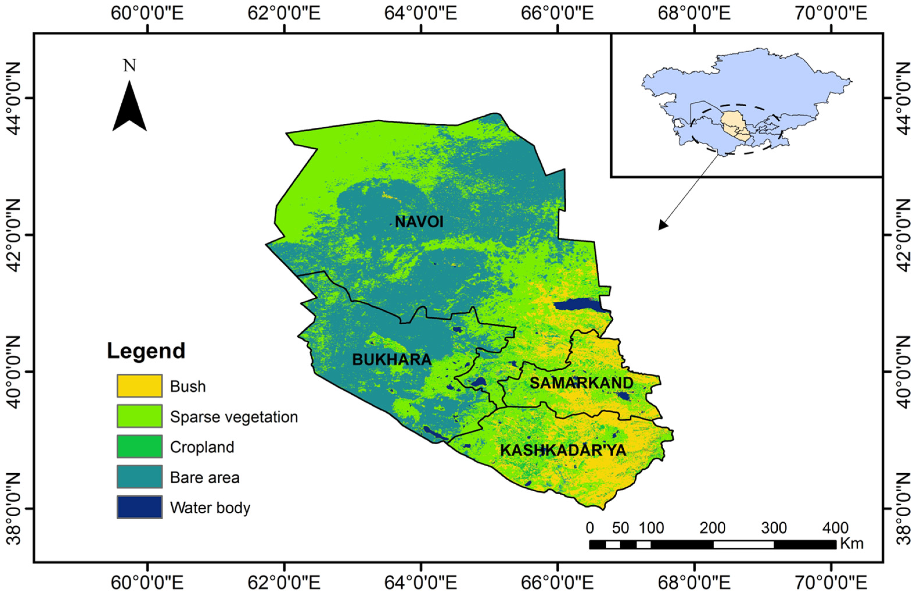
The Amu Darya River Basin (which ranges from 34°30′ to 43°45′ N in latitude, and from 58°15′ to 75°07′ E in longitude) is located in Central Asia [21,22]. The basin belongs to a semi-arid and a continental temperature climate zone, with an average temperature of about 13 °C and annual precipitation of 100 mm [23]. The study area located in the middle reaches of the Amu Darya River, covering an area of 196 × 10³ km², contains four districts (i.e., Bukhara, Kashkadarya, Navoi and Samarkand, as shown in Figure 2). The total population in the region is about 7.5 million, of which 56% is a rural population, and the agricultural economy accounts for about 45% of the regional GDP [24]. The water resources mainly come from surface water and groundwater. More than 70% of the water in irrigated agriculture is obtained from surface water, and the rest is from groundwater and other water sources [25]. Most of the domestic water is obtained from groundwater, of which urban water is 1.142 km³/a, and rural water is 1.423 km³/a [26]. Since the disintegration of the Soviet Union, with the development of industry, the increase in the population and the expansion of agriculture, the contradiction between the supply of and demand for water resources has intensified, especially the contradiction of the circulation of the surface and groundwater system. In general, with the overexploitation of groundwater and the inefficient use of surface water, it is indispensable for the water-resource manager to develop an effective joint-management approach to regional water resources to improve the utilization of water resources and promote the sustainable development of the economy and environment.

4. Development of the HFOP-SGW Model

Based on the proposed HFOP approach, a HFOP-SGW model was developed for the surface–groundwater (SGW) system, where four states and four water users were involved. The HFOP-SGW model aims to adjust the structure of water use and alleviate the contradiction between the supply of and demand for regional water resources. Thus the objective function can be formulated as:

$$\mathrm{Max}f=(1)+(2)+(3)+(4)-(5)$$

(42)

(1) Benefits from the industrial sectors

$${\displaystyle \sum _{k=1}^4(IN{W}_k^{\pm }+IN{G}_k^{\pm })}·BI{N}_k^{\pm }-{\displaystyle \sum _{k=1}^4{\displaystyle \sum _{h=1}^3{P}_h·CI{N}_k^{\pm }·(QI{N}_{kh}^{\pm }+QGI{N}_{kh}^{\pm }}})$$

(43)

(2) Benefits from the municipal sectors

$${\displaystyle \sum _{k=1}^4(MW{W}_k^{\pm }+MW{G}_k^{\pm })}·BM{W}_k^{\pm }-{\displaystyle \sum _{k=1}^4{\displaystyle \sum _{h=1}^3{P}_h·CM{W}_k^{\pm }·(QM{W}_{kh}^{\pm }+QGM{W}_{kh}^{\pm }}})$$

(44)

(3) Benefits from the agricultural sectors

$${\displaystyle \sum _{k=1}^4(AG{W}_k^{\pm }+AG{G}_k^{\pm })}·BA{G}_k^{\pm }-{\displaystyle \sum _{k=1}^4{\displaystyle \sum _{h=1}^3{P}_h·CA{G}_k^{\pm }·(QA{G}_{kh}^{\pm }+QGA{G}_{kh}^{\pm }}})$$

(45)

(4) Benefits from the ecological sectors

$${\displaystyle \sum _{k=1}^4(EC{W}_k^{\pm }+EC{G}_k^{\pm })}·BE{C}_k^{\pm }-{\displaystyle \sum _{k=1}^4{\displaystyle \sum _{h=1}^3{P}_h·CE{C}_k^{\pm }·(QE{C}_{kh}^{\pm }+QGE{C}_{kh}^{\pm }}})$$

(46)

(5) Cost of water transportation

$$\begin{array}{l}{\displaystyle \sum _{k=1}^4{\displaystyle \sum _{h=1}^3(IN{W}_k^{\pm }-P_h·QI{N}_{kh}^{\pm }})}·WI{N}_k^{\pm }+{\displaystyle \sum _{k=1}^4{\displaystyle \sum _{h=1}^3(IN{G}_k^{\pm }-P_h·QGI{N}_{kh}^{\pm })}·GI{N}_k^{\pm }}+\\ {\displaystyle \sum _{k=1}^4{\displaystyle \sum _{h=1}^3(MW{W}_k^{\pm }-P_h·QM{W}_{kh}^{\pm }})}·WM{W}_k^{\pm }+{\displaystyle \sum _{k=1}^4{\displaystyle \sum _{h=1}^3(MW{G}_k^{\pm }-P_h·QGM{W}_{kh}^{\pm })}·GM{W}_k^{\pm }}+\\ {\displaystyle \sum _{k=1}^4{\displaystyle \sum _{h=1}^3(AG{W}_k^{\pm }-P_h·QA{G}_{kh}^{\pm }})}·WA{G}_k^{\pm }+{\displaystyle \sum _{k=1}^4{\displaystyle \sum _{h=1}^3(AG{G}_k^{\pm }-P_h·QGA{G}_{kh}^{\pm })}·GA{G}_k^{\pm }}+\\ {\displaystyle \sum _{k=1}^4{\displaystyle \sum _{h=1}^3(EC{W}_k^{\pm }-P_h·QE{C}_{kh}^{\pm }})}·WE{C}_k^{\pm }+{\displaystyle \sum _{k=1}^4{\displaystyle \sum _{h=1}^3(EC{G}_k^{\pm }-P_h·QGE{C}_{kh}^{\pm })}·GE{C}_k^{\pm }}\end{array}$$

(47)

The constraints of the HFOP-SGW model can be characterized as follows:

(1) Constraint of surface-water-resource availability. The total allocated water amounts must be less than the availability of surface water in the region. The constraints are designed at different levels to reflect the randomness of surface-water availability.

$$\begin{array}{l}[{\displaystyle \sum _{k=1}^4(IN{W}_k^{\pm }-QI{N}_{kh}^{\pm })}+{\displaystyle \sum _{k=1}^4(IN{W}_k^{\pm }-QI{N}_{kh}^{\pm })}+\\ {\displaystyle \sum _{k=1}^4(IN{W}_k^{\pm }-QI{N}_{kh}^{\pm })}+{\displaystyle \sum _{k=1}^4(IN{W}_k^{\pm }-QI{N}_{kh}^{\pm })}]/(1-\alpha )\le DB{P}_h^{\pm }\forall h\end{array}$$

(48)

(2) Constraint of groundwater-resource availability.

The total groundwater supply to each region must not exceed the total availability of groundwater. Different levels of total availability of groundwater are to reflect the randomness of groundwater availability.

$$\begin{array}{l}(IN{G}_k^{\pm }-QGI{N}_{kh}^{\pm })+(MW{G}_k^{\pm }-QGM{W}_{kh}^{\pm })+\\ (AG{G}_k^{\pm }-QGA{G}_{kh}^{\pm })+(EC{G}_k^{\pm }-QGE{C}_{kh}^{\pm })\le \beta ·DX{P}_{kh}^{\pm }\forall k,h\end{array}$$

(49)

(3) Constraint of the quantity of wastewater.

The quantity of regional wastewater must be satisfied with the regional discharge standards. The amount of sewage generated in the area cannot exceed the environmental safety threshold. Such a constraint is set as fuzzy inequality to reflect the policy’s subjectivity and decision-makers’ attitudes toward environmental security.

$$\begin{array}{l}[(IN{G}_k^{\pm }-QGI{N}_{kh}^{\pm })+(IN{W}_{kt}^{\pm }-QI{N}_{kh}^{\pm })]·\xi +[(MW{G}_k^{\pm }-QGM{W}_{kh}^{\pm })\\ +(MW{W}_k^{\pm }-QM{W}_{kh}^{\pm })]·\zeta \le CL{S}_k^{\pm }+\left({\tau }_{\left(2\right)}+\frac{{\vartheta }_{\tau }-{\vartheta }_{\tau }^{\prime }}{3}\right)·\left(1-\gamma \right)\forall k,h\end{array}$$

(50)

(4) Constraint of water consumption of different water-user sectors.

The water-supply amount to water users in each district must not be less than the lowest water-consumption rate.

$$(IN{G}_k^{\pm }-QGI{N}_{kh}^{\pm })+(IN{W}_k^{\pm }-QI{N}_{kh}^{\pm })\ge IND{W}_k^{\pm }\forall k,h$$

(51)

$$(MW{G}_k^{\pm }-QGM{W}_{kh}^{\pm })+(MW{W}_k^{\pm }-QM{W}_{kh}^{\pm })\ge MWD{W}_k^{\pm }\forall k,h$$

(52)

$$(AG{G}_k^{\pm }-QGA{G}_{kh}^{\pm })+(AG{W}_k^{\pm }-QA{G}_{kh}^{\pm })\ge AGD{W}_k^{\pm }\forall k,h$$

(53)

$$(EC{G}_k^{\pm }-QGE{C}_{kh}^{\pm })+(EC{W}_k^{\pm }-QE{C}_{kh}^{\pm })\ge ECD{W}_k^{\pm }\forall k,h$$

(54)

(5) Non-negative constraint.

$$IN{W}_k,IN{G}_k,MW{W}_k,MW{G}_k,AG{W}_k,AG{G}_k,EC{W}_k,EC{G}_k\ge 0$$

(55)

In this study, 125 representative scenarios (as shown in

Table 1. Scenarios with different factor levels.

	α	β	γ		α	β	γ		α	β	γ		α	β	γ
S1	L	L	L	S33	ML	ML	M	S65	M	M	H	S97	MH	H	ML
S2	L	L	ML	S34	ML	ML	MH	S66	M	MH	L	S98	MH	H	M
S3	L	L	M	S35	ML	ML	H	S67	M	MH	ML	S99	MH	H	MH
S4	L	L	MH	S36	ML	M	L	S68	M	MH	M	S100	MH	H	H
S5	L	L	H	S37	ML	M	ML	S69	M	MH	MH	S101	H	L	L
S6	L	ML	L	S38	ML	M	M	S70	M	MH	H	S102	H	L	ML
S7	L	ML	ML	S39	ML	M	MH	S71	M	H	L	S103	H	L	M
S8	L	ML	M	S40	ML	M	H	S72	M	H	ML	S104	H	L	MH
S9	L	ML	MH	S41	ML	MH	L	S73	M	H	M	S105	H	L	H
S10	L	ML	H	S42	ML	MH	ML	S74	M	H	MH	S106	H	ML	L
S11	L	M	L	S43	ML	MH	M	S75	M	H	H	S107	H	ML	ML
S12	L	M	ML	S44	ML	MH	MH	S76	MH	L	L	S108	H	ML	M
S13	L	M	M	S45	ML	MH	H	S77	MH	L	ML	S109	H	ML	MH
S14	L	M	MH	S46	ML	H	L	S78	MH	L	M	S110	H	ML	H
S15	L	M	H	S47	ML	H	ML	S79	MH	L	MH	S111	H	M	L
S16	L	MH	L	S48	ML	H	M	S80	MH	L	H	S112	H	M	ML
S17	L	MH	ML	S49	ML	H	MH	S81	MH	ML	L	S113	H	M	M
S18	L	MH	M	S50	ML	H	H	S82	MH	ML	ML	S114	H	M	MH
S19	L	MH	MH	S51	M	L	L	S83	MH	ML	M	S115	H	M	H
S20	L	MH	H	S52	M	L	ML	S84	MH	ML	MH	S116	H	MH	L
S21	L	H	L	S53	M	L	M	S85	MH	ML	H	S117	H	MH	ML
S22	L	H	ML	S54	M	L	MH	S86	MH	M	L	S118	H	MH	M
S23	L	H	M	S55	M	L	H	S87	MH	M	ML	S119	H	MH	MH
S24	L	H	MH	S56	M	ML	L	S88	MH	M	M	S120	H	MH	H
S25	L	H	H	S57	M	ML	ML	S89	MH	M	MH	S121	H	H	L
S26	ML	L	L	S58	M	ML	M	S90	MH	M	H	S122	H	H	ML
S27	ML	L	ML	S59	M	ML	MH	S91	MH	MH	L	S123	H	H	M
S28	ML	L	M	S60	M	ML	H	S92	MH	MH	ML	S124	H	H	MH
S29	ML	L	MH	S61	M	M	L	S93	MH	MH	M	S125	H	H	H
S30	ML	L	H	S62	M	M	ML	S94	MH	MH	MH
S31	ML	ML	L	S63	M	M	M	S95	MH	MH	H
S32	ML	ML	ML	S64	M	M	MH	S96	MH	H	L

) with five surface-water-transmission loss-rate levels (i.e., α = L (0.22), ML (0.24), M (0.26), MH (0.28) and H (0.30)), five groundwater abstraction-rate levels (i.e., β = L (0.40), ML (0.42), M (0.44), MH (0.46) and H (0.48)) and five satisfaction decision levels (i.e., γ = L (0.2), ML (0.4), M (0.6), MH (0.8) and H (1)) were examined through factorial designs. The factorial combinations were designed by Minitab, and the optimization model was programmed by Lingo. The variables and parameters of the HFOP-SGW model are clearly listed at the end of the paper.

Water availability (as shown in

Table 2. Water availability at different flow levels (10⁶ m³).

Water Source	Flow Level	Probability	Water Availability
Groundwater	Low	0.2	[3655, 3887]
	Medium	0.6	[4037, 4269]
	High	0.2	[4676, 4908]
Surface water	Low	0.2	[6822, 7476]
	Medium	0.6	[8357, 9011]
	High	0.2	[9057, 9712]

) was obtained by referring to the hydrological site flows, statistical yearbooks, literature data and related statistical websites. The water-supply target for different water users (as shown in

Table 3. Water-allocation target for different users (10⁶ m³).

Water Source	District	Users
		Industrial	Municipal	Agricultural	Ecological
Groundwater	Bukhara	[24.9, 37.8]	[23, 50.6]	[85.1, 112.9]	[22.0, 28.6]
	Kashkadarya	[17.6, 28.6]	[152.6, 191.6]	[524.3, 651.5]	[31.8, 37.3]
	Navoi	[16.6, 24.0]	[26.4, 33.2]	[61.6, 71.5]	[22.0, 31.7]
	Samarkand	[37.2, 45.0]	[494, 573.9]	[331.1, 379.7]	[23.5, 32.2]
Surface water	Bukhara	[44.0, 128.0]	[46.0, 127]	[1317.0, 1663.0]	[160.0, 377.0]
	Kashkadarya	[180.0, 332]	[132, 310]	[1085.0, 1565.0]	[440.0, 700.0]
	Navoi	[690.0, 920.0]	[45.0, 127.0]	[1106.0, 1456.0]	[108.0, 164.0]
	Samarkand	[45.0, 131.0]	[235.0, 289.0]	[912.0, 1245.0]	[355.0, 475.0]

) was collected from the Central Asia Water Resources Information Website (http://www.cawater-info.net/ (accessed on 5 October 2021)). The data related to socio-economic factors (unit water benefit, population and yield of food crops per unit area), water resources and agriculture. For example, the benefit for water users, the penalty for water waste and the cost of water delivery (as shown in

Table 4. Economic parameters used in the optimization model (USD/m³).

Distract	User
	Industrial	Municipal	Agricultural	Ecological
Net benefit when water-allocation target is satisfied (USD/m3)
Bukhara	[11.0, 13.2]	[7.0, 7.2]	[1.7, 1.8]	[2.0, 2.2]
Kashkadarya	[10.1, 12.2]	[8.2, 8.5]	[2.1, 2.3]	[1.5, 1.7]
Navoi	[9.3, 11.5]	[6.3, 7.3]	[2.4, 2.5]	[1.2, 1.4]
Samarkand	[10.7, 12.6]	[7.0, 8.2]	[1.6, 1.9]	[1.4, 1.6]
Penalty when water is not delivered (USD/m3)
Bukhara	[15.8, 18.2]	[14.4, 16.4]	[5.0, 5.7]	[3.4, 3.8]
Kashkadarya	[14.6, 16.3]	[17.2, 18.7]	[8.0, 9.1]	[2.7, 3.1]
Navoi	[13.8, 15.7]	[14.6, 16.2]	[7.0, 8.1]	[2.2, 2.5]
Samarkand	[15.1, 16.8]	[16.4, 18.1]	[8.1, 8.9]	[2.5, 2.8]

) were collected through practical investigations, expert inquiries, the statistical yearbooks of Uzbekistan (2013–2019) and the literature reports. All the figures presented above are revised according to the actual conditions, water demand and policy changes.

5. Results and Discussion

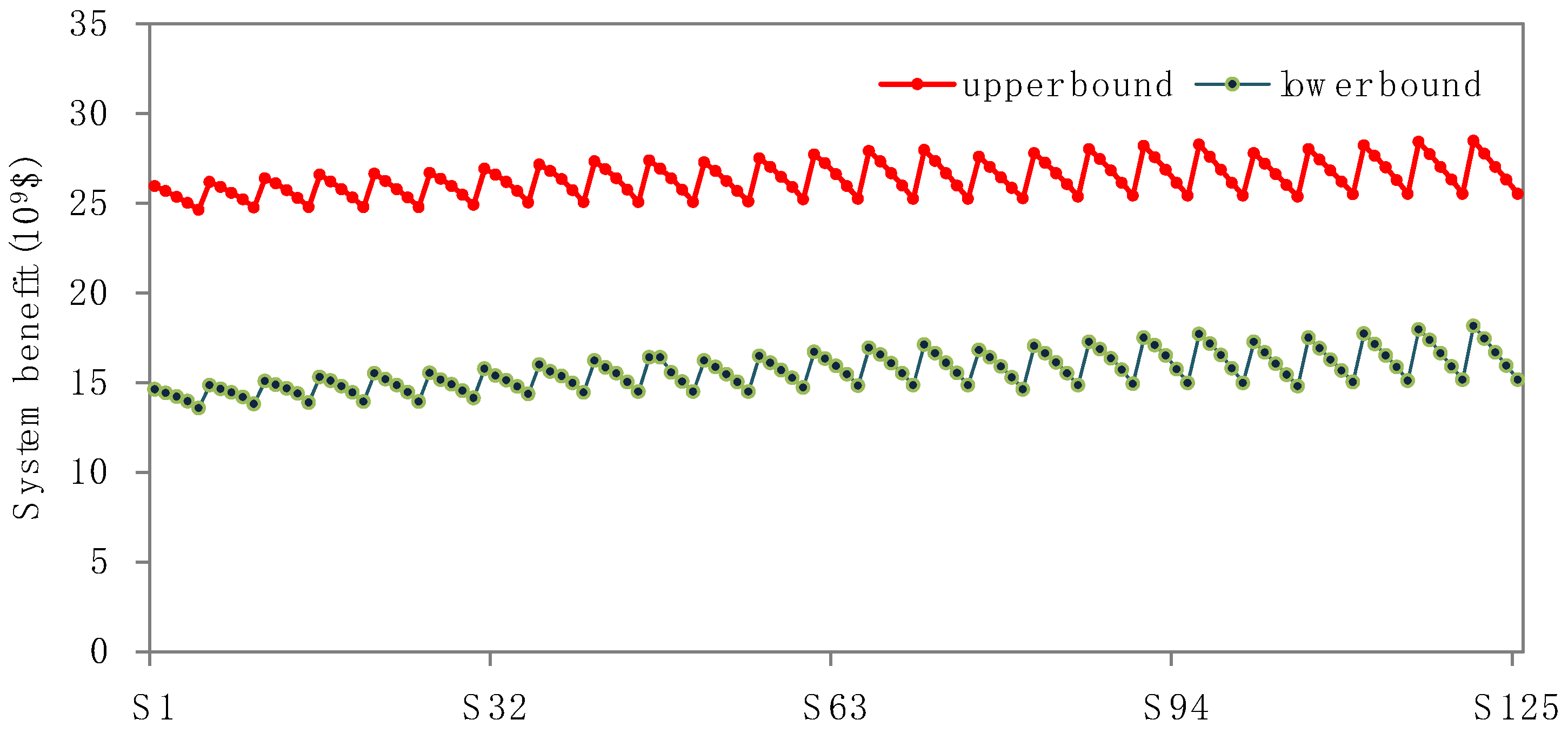
Figure 3 provides the results for the system’s benefits for 125 scenario combinations designed, based on different factor levels. The results indicate that different combinations of factor levels would bring about a change in the system’s benefits. The system’s benefits range from USD [13.58, 24.64] × 10⁹ (in the α = 0.30, β = 0.40, γ = 1, scenario S5) to USD [18.16, 28.47] × 10⁹ (in the α = 0.22, β = 0.48, γ = 0.2, scenario S121). More specifically, a higher γ level can lead to a lower system benefit. The reason for this is that the γ level reflects the decision-maker’s attitude towards risk, the high γ level represents the decision-maker’s lowest tolerance for systematic risks, and the low γ level represents the decision-maker’s optimistic attitude towards risks. Additionally, in the optimistic decision-making scenario, when β = 0.48, γ = 0.2, the system’s benefit is USD [16.42, 27.39] × 10⁹ when α = 0.28 and USD [17.70, 28.26] × 10⁹ when α = 0.24. Higher α levels lead to a lower system benefit. The main reason is that α represents the water-delivery loss rate of the system, the high α level represents a high water-delivery loss rate and the low efficiency of the water-delivery infrastructure, and the low α level reflects an effective water-delivery infrastructure. Improving the efficiency level of the water-delivery facility can significantly improve the system’s benefits and ensure regional stability.

Table 5. Optimized water-allocation targets for different users in S121 (10⁶ m³).

Water Source	User	Distract
		Bukhara	Kashkadarya	Navoi	Samarkand
Groundwater	Industrial	35.2	26.9	18.2	42.5
	Municipal	23.0	152.6	26.4	494
	Agricultural	85.1	524.3	61.6	331.1
	Ecological	27.1	32.2	22.0	23.5
Surface water	Industrial	113.9	301.0	825.3	117.4
	Municipal	46.0	155.8	45.0	235.0
	Agricultural	1317.0	1085.0	1106.0	912.0
	Ecological	160.0	440.0	108.0	355.0

shows the solutions of optimized water-allocation targets for different water users in the planning horizon in the high-system-benefit scenario (S121). The results indicate that numbers of water-allocation targets to water users have been adjusted for ensuring the stability of the system and obtaining the optimal water-resource allocation scheme. With the known water-flow level, the water deficits for water users can be optimized for decreasing the system’s losses. For instance, the initial groundwater-allocation target for an industrial user from Bukhara was [24.9, 37.8] × 10⁶ m³; through solving the model, the optimal value was 35.2 × 10⁶ m³. The variations of water-allocation targets for different water users reflected the resilience to water-resource fluctuations and policy changes. When the water-allocation target reached the upper bound, the SGW system would be in a high-risk situation due to the serious water shortage under low or medium water levels. In general, solving the model can further optimize the allocation of water resources, balance the system’s benefits and mitigate water shortages.

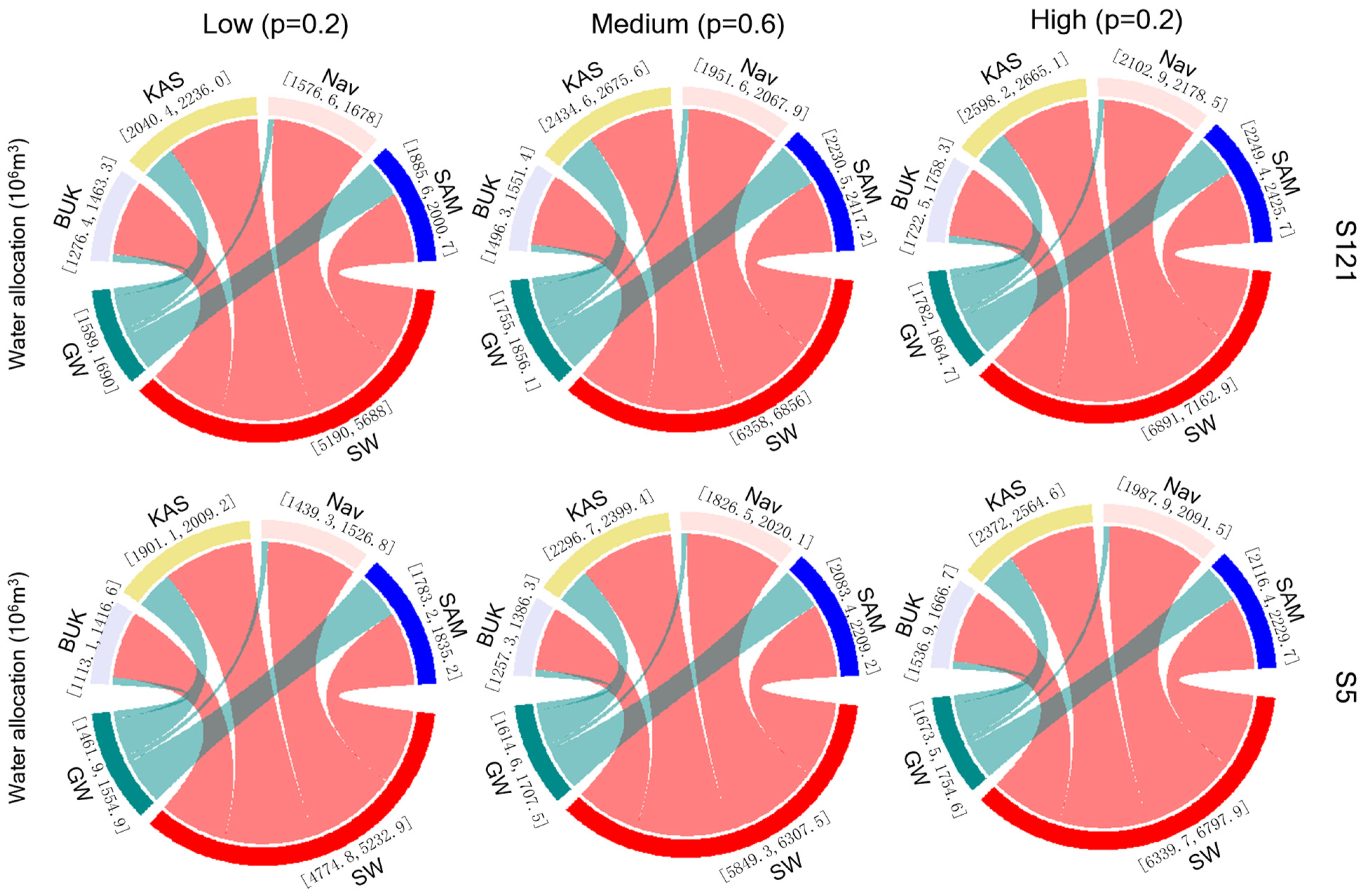
Figure 4 shows the patterns of water-allocation targets in different regions in the high-system-benefit (S121) and low-system-benefit (S5) scenarios over the planning horizon. The results indicate that the water-allocation targets greatly vary in the four states in different scenarios. More specifically, Kashkadarya (KAS) accounts for the highest water-allocation target and Bukhara (BUK) accounts for the lowest among all three water-flow levels. For instance, at a low-flow level, the water-allocation target for Kashkadarya (KAS) is about [2040.4, 2236.0] × 10⁶ m³ in S121, accounting for 30.3~30.5% of the total water resource (surface water and groundwater), and the water-allocation target for Bukhara (BUK) is about [1276.4, 1463.3] × 10⁶ m³, accounting for 19.1~19.8% of the total water resource (surface water and groundwater). The main reason is that agriculture is an important part of the economic structure of Kashkadarya, including grain planting, animal husbandry and cotton production, which consume a lot of water resources. On the contrary, the economies of Bukhara mainly include the fine processing of agricultural products and the processing of building materials, which consume less water resources. In general, the higher the water demand of the state, the more sensitive it is to change in different scenarios, and it is more necessary to adjust the scale of water use or improve the efficiency of water use according to the actual situation.

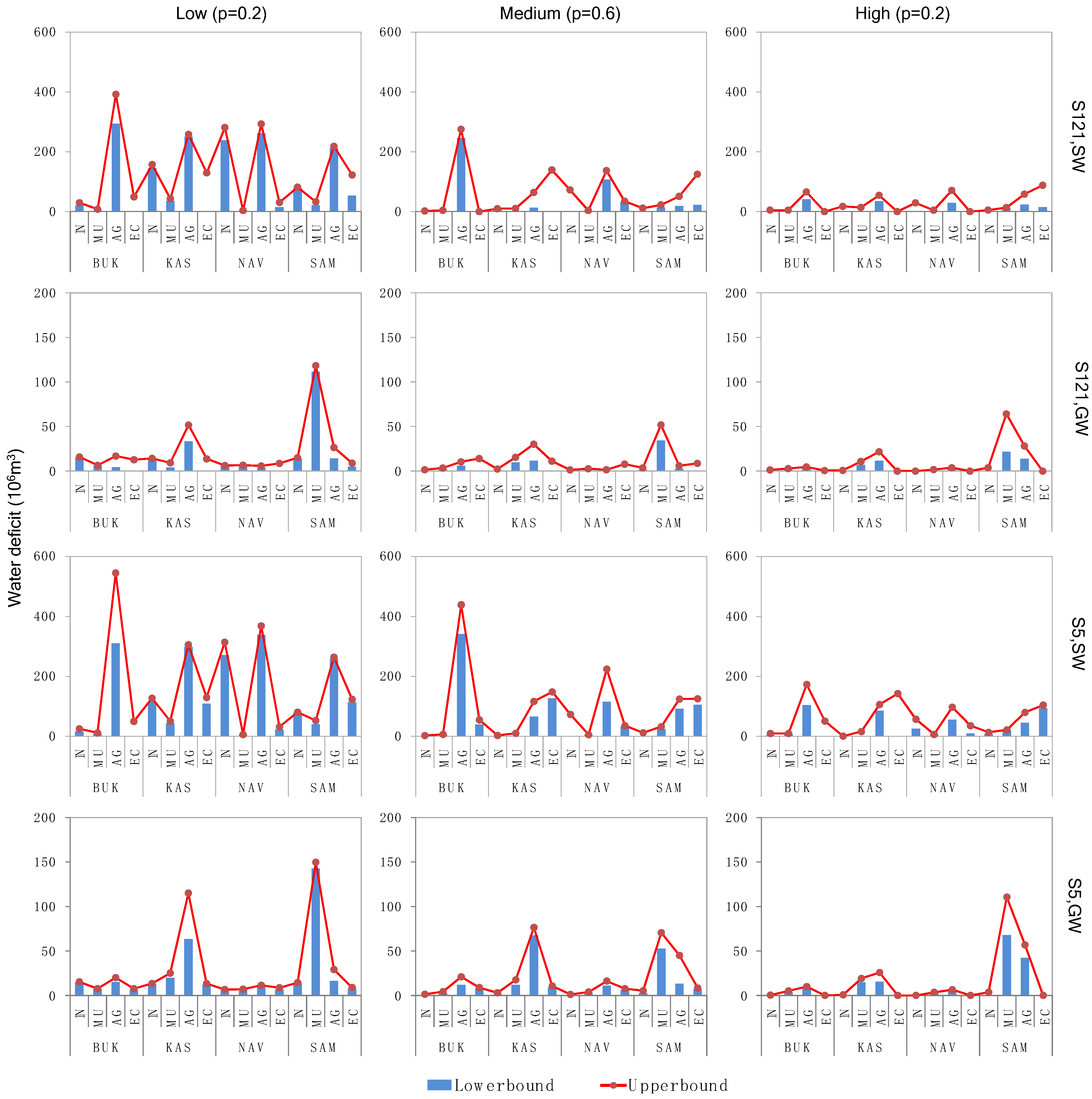
Figure 5 presents the water deficits of water users in different scenarios. The results indicate that there is a serious water-shortage problem in the study area, and there are significant differences in water the shortage levels among water users. The statistical results of various water shortages show that about 19.5%~25.8% of the water-resource targets cannot be met at low levels. The main reasons for this situation are the unreasonable water structure and serious water loss in Central Asia. It can be observed from the results that there are great differences in the water shortage levels among water users, among which agricultural users of surface water have the greatest water shortage loss, and groundwater is the largest for municipal water shortages. For example, under a low water-flow level, the water-deficit ratios for agricultural users of groundwater and surface water are [5.5, 10.1]% and [23.1, 26.2]%, respectively; the water-deficit ratios for municipal users of groundwater and surface water are [18.3, 20.2]% and [13.4, 18.2]%, respectively, in a high-benefit scenario (S121). The reason for this is that more than 80% of agricultural water in Central Asia is obtained from surface water, so agricultural users are more sensitive to surface-water fluctuations and have a high probability of water shortages. Correspondingly, municipal water is mainly obtained from groundwater, which is greatly affected by the fluctuation of water sources.

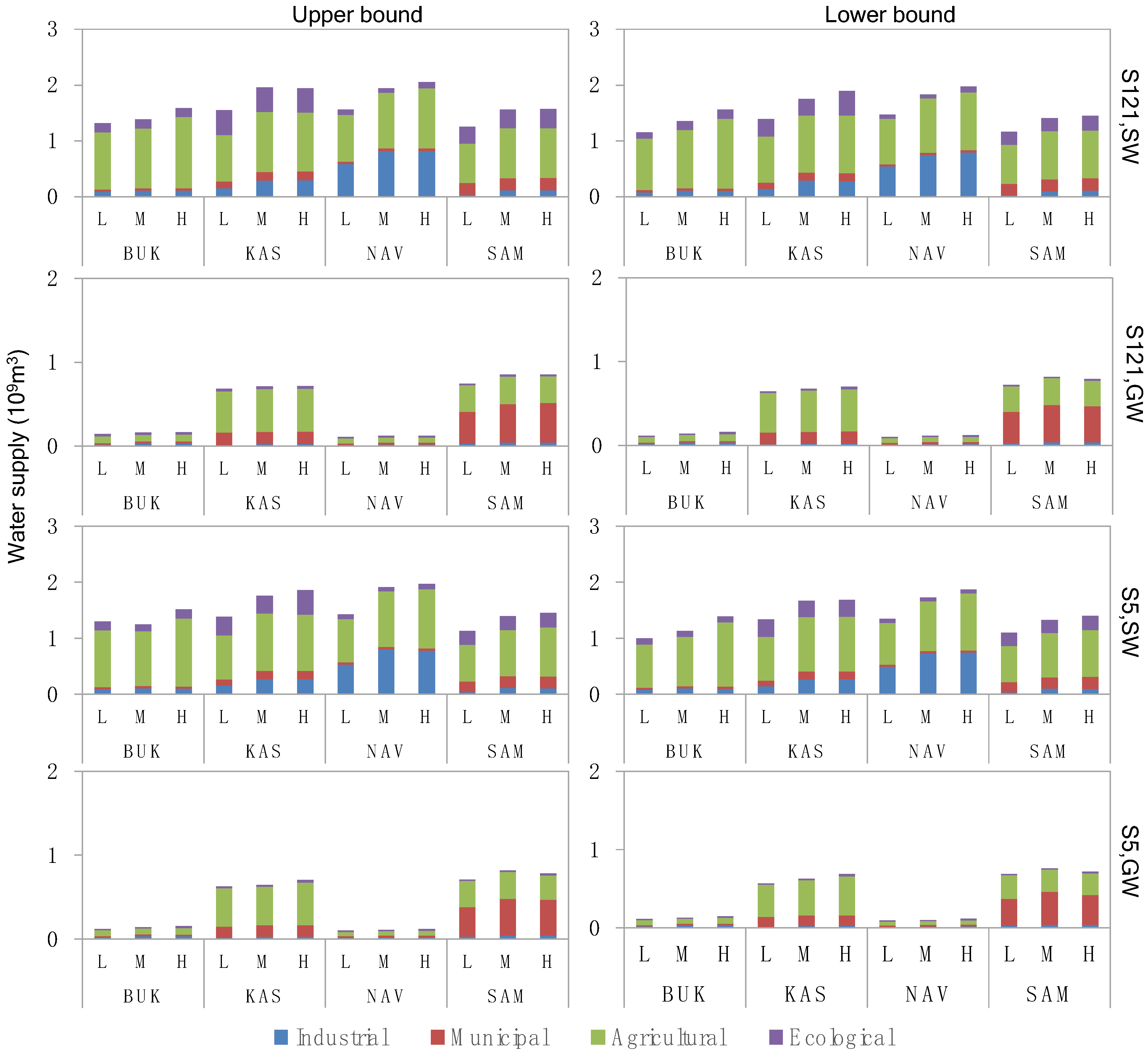
Figure 6 depicts the solutions of the optimized water-resource allocation scheme for water users in different scenarios (high-benefit (S121) and low-benefit (S5) scenarios) obtained from the HFOP-SGW model. The results show that the water-resource allocation patterns are closely related to the regional water-use structure and economic policy. In detail, agricultural users are in the highest position to be adjusted for water demand when water security and emergency development need to be guaranteed. For instance, at a low-flow level, the water supply of surface water for agriculture in Bukhara is [924, 1023] × 10⁶ m³, in S121; at a high-flow level, the value would be [1250, 1275] × 10⁶ m³. This is because irrigated agriculture possesses high water requirements and low economic benefits. Different water-supply schemes are generated according to the water-resource demands of water users. The results show that in various scenarios, the demand for municipal water mainly comes from groundwater. Under different inflow levels, municipal water is most sensitive to groundwater availability. The main reason for this is the high salinity of surface water in Central Asia.

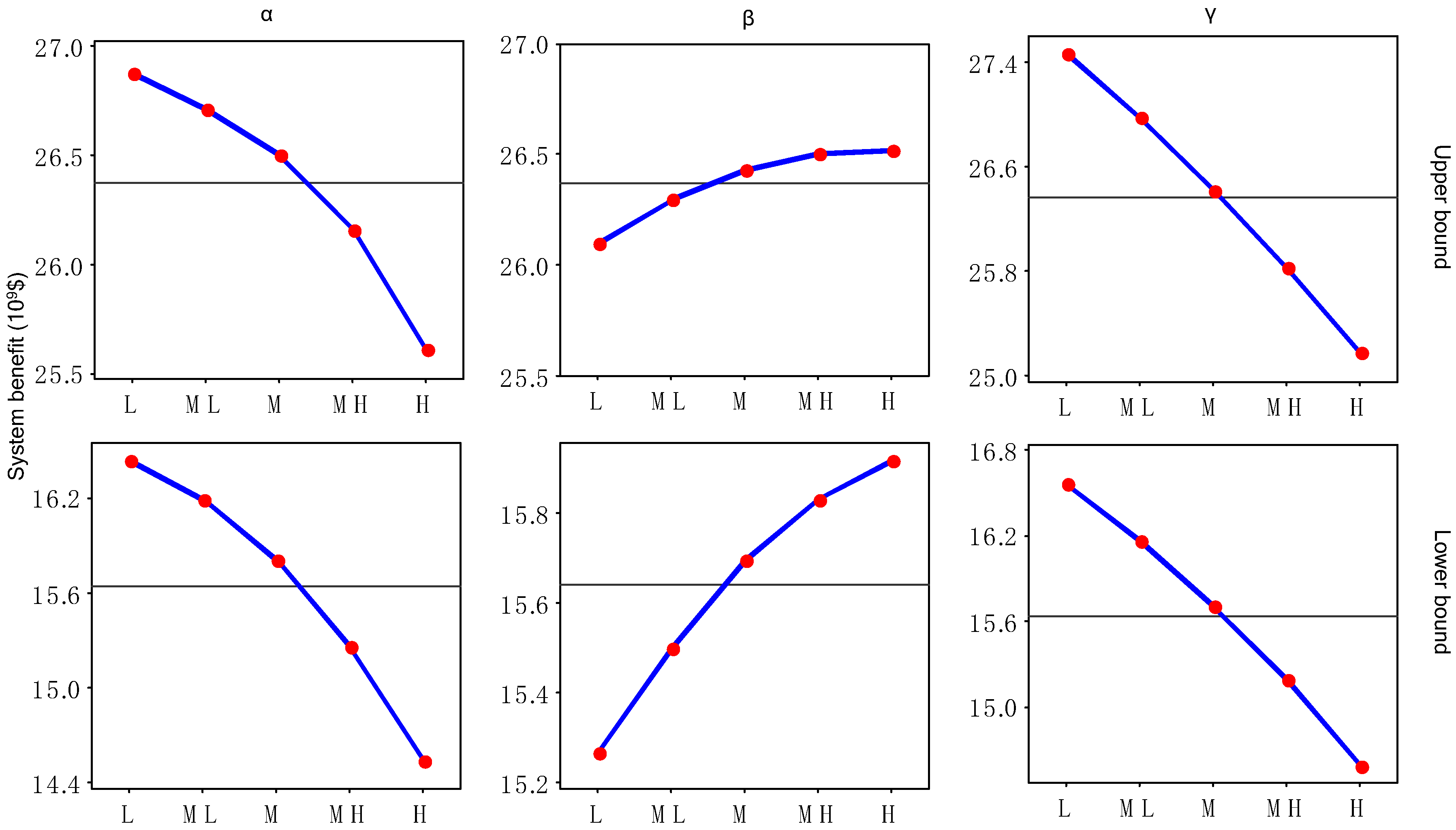
Figure 7 shows the effects of multiple parameters on the system’s benefits. Combinatorial designs of multiple factors can support the analysis of the interaction of the model parameters (e.g., α, β and γ). The results indicate that the surface-water-transmission loss rate (α) and the satisfaction decision level (γ) have a negative effect on the system’s benefits; the groundwater abstraction-rate (β) has a positive effect on the system’s benefits. For example, when α increases from a low to a high level, the system’s benefit decreases by about USD 1.3 × 10⁹ in the upper bound; when β increases from a low to a high level, the system’s benefit increases by about USD 0.4 × 10⁹ in the upper bound. The change reflects the fact that factor α has a greater impact on the system’s performance than factor β. In detail, as described in

Table 6. Contributions of the individual and interactive factors.

Factor	Percentage of Contribution	p-Value
Main effect
α	33.272%	<0.05
β	3.987%	<0.05
γ	59.338%	<0.05
Interactive effect
α × β	0.007%	<0.05
α × γ	2.759%	<0.05
β × γ	0.609%	<0.05
α × β × γ	0.028%	<0.05

, the contributions of the surface-water-transmission loss rate (α), groundwater abstraction-rate (β) and satisfaction decision level (γ) are 33.272%, 3.987% and 59.338%, respectively. The results indicate that the surface-water-transmission loss rate (α) and confidence level (γ) are the main factors that affect the system’s benefits. The reason is that the excessive use of surface water in the study area exacerbates the impact of water-delivery facilities on the system’s stability. In general, improving the water-delivery efficiency of surface water and the water-use structure is a necessary way to maintain regional stability and achieve a high system benefit.

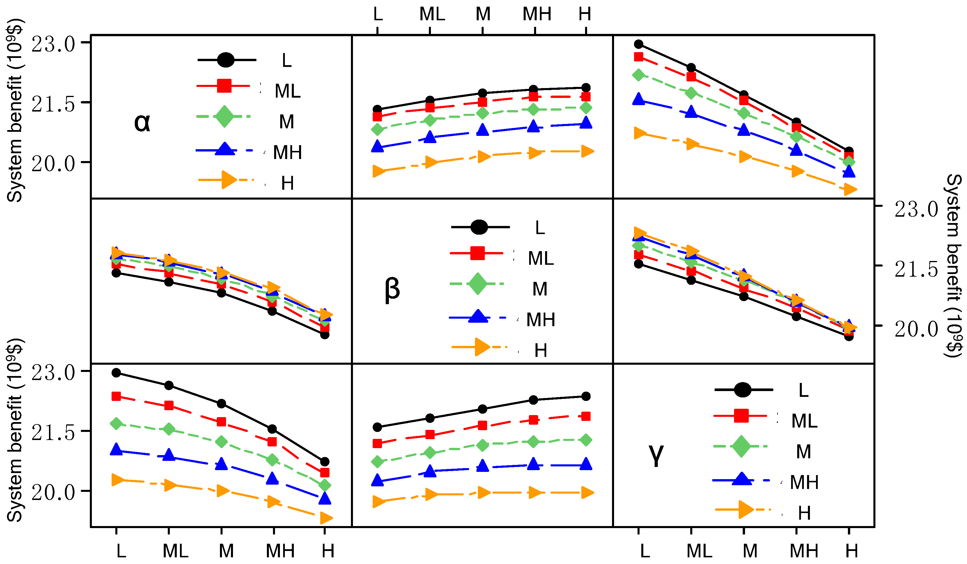
Figure 8 presents the interactive effects of multiple parameters on the system’s benefits. The results indicate that the interaction of the surface-water-transmission loss rate (α) and satisfaction decision level (γ) has a significant effect on the system’s benefits. For instance, when the surface-water-transmission loss rate is at a high level, the system’s benefits decrease from USD 20.7 × 10⁹ to USD 19.3 × 10⁹, with the satisfaction decision level (γ) increasing from a low (L) to a high (H) level; when the surface-water-transmission loss rate is at a low level, the system’s benefits decrease from USD 22.9 × 10⁹ to USD 20.3 × 10⁹, with the satisfaction decision level (γ) increasing from a low (L) to a high (H) level. The results show that there is a close relationship between the level of regional economic development and environmental sustainable development. In detail, the interactive contribution between the surface-water-transmission loss rate (α) and the satisfaction decision level (γ) has a more significant impact on the system’s benefits than the other interactive contributions. As shown in Table 6, the interactive contribution between the surface-water-transmission loss rate (α) and satisfaction decision level (γ) is about 2.759%, and the interactive contribution between the groundwater-restriction rate (β) and the satisfaction decision level (γ) is about 0.609%. The results indicate that decision making needs to comprehensively consider the water-distribution plan to achieve economic growth and environmental health, according to the needs of sustainable development.

6. Conclusions

In the present study, a hybrid factorial optimization programming (HFOP) method was developed by integrating factorial analysis, interval linear programming, flexible fuzzy programming and two-stage stochastic programming into a general framework. HFOP can not only reflect the uncertainties expressed as probability distributions and interval values, but also effectively address the fuzzy-decision problem. Through applying the HFOP method to the SGW system, a HFOP-SGW model was developed for the middle reach of the Amu Darya River Basin, and multiple scenarios corresponding to the different parameter levels were examined. Issues of surface-water use, groundwater protection and water-pollution control were considered in the modeling process. The HFOP-SGW model can make a tradeoff between the system’s benefits and water consumption under multiple uncertainties. Additionally, the quantitative analysis of parameter relationships can help decision makers to identify the main parameters and understand the interaction between those parameters.

The solutions of the HFOP-SGW model in different combined scenarios were obtained. Some of the findings can be concluded as follows: (i) the improvement of surface-water-transport efficiency and the proper use of groundwater can effectively alleviate regional water shortages; (ii) agricultural users have the highest risk of water scarcity of all states, especially under a low-flow level (the water-deficit ratios of agriculture for surface water are [23.1, 26.2]% (in S121)); (iii) the uncertainties of water-flow levels and risk-reverse attitudes of decision makers have a significant impact on the system’s benefits and water-resource allocation scheme; and (iv) the surface-water-transmission loss rate and risk perceptions of decision makers are the main factors affecting the system’s benefits and water-allocation scheme. HFOP is an effective tool for addressing the water-allocation problem in the SGW system. However, the developed method is a single-objective decision-making method based on linear programming, which has difficulty in solving the multi-objective problem. A more robust programming method can be developed to the optimization framework for enhancing its capability of dealing with multilevel-decision problems, such as multi-objective programming and bi-level programming.

References

- Chen, S.; Tan, Y.; Liu, Z. Direct and embodied energy-water-carbon nexus at an inter-regional scale. Appl. Energy 2019, 251, 113401. [Google Scholar] [CrossRef]
- Ji, L.; Zhang, B.; Huang, G.; Lu, Y. Multi-stage stochastic fuzzy random programming for food-water-energy nexus management under uncertainties. Resour. Conserv. Recycl. 2020, 155, 104665. [Google Scholar] [CrossRef]
- Panyushkina, I.P.; Meko, D.M.; Macklin, M.G.; Toonen, W.; Mukhamadiev, N.S.; Konovalov, V.G.; Ashikbaev, N.Z.; Sagitov, A.O. Runoff variations in lake balkhash basin, central asia, 1779–2015, inferred from tree rings. Clim. Dyn. 2018, 51, 3161–3177. [Google Scholar] [CrossRef]
- Guo, H.; Bao, A.; Liu, T.; Jiapaer, G.; Maeyer, P.D. Spatial and temporal characteristics of droughts in Central Asia during 1966–2015. Sci. Total Environ. 2018, 624, 1523–1538. [Google Scholar] [CrossRef] [PubMed]
- Gulahmadov, N.; Chen, Y.; Gulakhmadov, A.; Rakhimova, M.; Gulakhmadov, M. Quantifying the Relative Contribution of Climate Change and Anthropogenic Activities on Runoff Variations in the Central Part of Tajikistan in Central Asia. Land 2021, 10, 525. [Google Scholar] [CrossRef]
- Huggins, X.; Gleeson, T.; Eckstrand, H.; Kerr, B. Streamflow depletion modeling: Methods for an adaptable and conjunctive water management decision support tool. JAWRA J. Am. Water Resour. Assoc. 2018, 54, 1024–1038. [Google Scholar] [CrossRef]
- Zipper, S.C.; Gleeson, T.; Li, Q.; Kerr, B. Comparing Streamflow Depletion Estimation Approaches in a Heavily Stressed, Conjunctively Managed Aquifer. Water Resour. Res. 2021, 57. [Google Scholar] [CrossRef]
- Sepahvand, R.; Safavi, H.R.; Rezaei, F. Multi-objective planning for conjunctive use of surface and ground water resources using genetic programming. Water Resour. Manag. Int. J. 2019, 33, 2123–2137. [Google Scholar] [CrossRef]
- Abbas, A.; Mina, K.; Leila, O.; Amin, A. Reliability-based multi-objective optimum design of nonlinear conjunctive use problem; cyclic storage system approach—Sciencedirect. J. Hydrol. 2020, 588, 125109. [Google Scholar]
- Qiao, Z.; Ma, L.; Liu, T.; Huang, X. An ecological stability-oriented model for the conjunctive allocation of surface water and groundwater in oases in arid inland river basins. Water Sci. Technol. Water Supply 2020, 21, 368–385. [Google Scholar] [CrossRef]
- Daneshvar, M.; Mohammadi-Ivatloo, B.; Zare, K.; Asadi, S. Two-stage stochastic programming model for optimal scheduling of the wind-thermal-hydropower-pumped storage system considering the flexibility assessment. Energy 2020, 193, 116657. [Google Scholar] [CrossRef]
- Nikzad, E.; Bashiri, M.; Oliveira, F. Two-stage stochastic programming approach for the medical drug inventory routing problem under uncertainty—Sciencedirect. Comput. Ind. Eng. 2019, 128, 358–370. [Google Scholar] [CrossRef]
- Borges, P.; Sagastizábal, C.; Solodov, M. A regularized smoothing method for fully parameterized convex problems with applications to convex and nonconvex two-stage stochastic programming. Math. Program. 2021, 189, 117–149. [Google Scholar] [CrossRef]
- Ma, Y.; Li, Y.P.; Huang, G.H.; Liu, Y.R. Water-energy nexus under uncertainty: Development of a hierarchical decision-making model. J. Hydrol. 2020, 591, 125297. [Google Scholar] [CrossRef]
- Niu, T.; Yin, H.; Feng, E. Economic and flexible design under uncertainty for steam power systems based on interval two-stage stochastic programming. Ind. Eng. Chem. Res. 2021, 60, 4019–4029. [Google Scholar] [CrossRef]
- Pishvaee, M.S.; Khalaf, M.F. Novel robust fuzzy mathematical programming methods. Appl. Math. Model. 2016, 40, 407–418. [Google Scholar] [CrossRef]
- Birge, J.R.; Louveaux, F.V. A multicut algorithm for two-stage stochastic linear programs. Eur. J. Oper. Res. 1988, 34, 384–392. [Google Scholar] [CrossRef] [Green Version]
- Huang, G.H. A hybrid inexact-stochastic water management model. Eur. J. Oper. Res. 1998, 107, 137–158. [Google Scholar] [CrossRef]
- Yager, R.R. A procedure for ordering fuzzy subsets of the unit interval. Inf. Sci. 1981, 24, 143–161. [Google Scholar] [CrossRef]
- Huang, G.H.; Baetz, B.W.; Patry, G.G. A grey linear programming approach for municipal solid waste management planning under uncertainty. Civ. Eng. Environ. Syst. 1992, 9, 319–335. [Google Scholar] [CrossRef]
- Mergili, M.; Mueller, J.P.; Schneider, J.F. Spatio-temporal development of high-mountain lakes in the headwaters of the Amu Darya river (central Asia). Glob. Planet. Chang. 2013, 107, 13–24. [Google Scholar] [CrossRef]
- Sun, J.; Li, Y.P.; Suo, C.; Liu, Y.R. Impacts of irrigation efficiency on agricultural water-land nexus system management under multiple uncertainties—A case study in Amu Darya River basin, Central Asia. Agric. Water Manag. 2019, 216, 76–88. [Google Scholar] [CrossRef]
- Salehie, O.; Ismail, T.; Shahid, S.; Sammen, S.S.; Wang, X. Selection of the Gridded Temperature Dataset for Assessment of Thermal Bioclimatic Environment Changes in Amu Darya River Basin. Stoch. Environ. Res. Risk Assess. 2022. online ahead of print. [Google Scholar] [CrossRef] [PubMed]
- Khushnud, Z.; Tokhir, S.; Zhou, Q.; Yang, H. Analyzing Characteristics and Trends of Economic Growth in the Sectors of National Economy of Uzbekistan. In Proceedings of the 4th International Symposium on Business Corporation and Development in South-East and South Asia under B&R Initiative (ISBCD 2019), Kunming, China, 24 November 2019. [Google Scholar]
- Uzbekov, U.; Bokhir, A. A review of water resource management considering climate change impacts in Uzbekistan. Sustain. Agric. 2019, 2, 40–42. [Google Scholar]
- Kulmatov, R.; Taylakov, A.; Khasanov, S. Investigating and evaluating the dynamics of change in water resources of the Aydar-Arnasay lake system in Uzbekistan. Environ. Sci. Pollut. Res. 2021, 28, 12245–12255. [Google Scholar] [CrossRef] [PubMed]
Figure 1.
The framework of this study.
Figure 2.
Study area.
Figure 3.
System’s benefits in different scenarios.
Figure 4.
The patterns of water-allocation targets in different regions.
Figure 5.
The water deficits of water users in different scenarios.
Figure 6.
The water-supply schemes for water users in different scenarios.
Figure 7.
Main effects of multiple parameters on the system’s benefits.
Figure 8.
Interactive effects of multiple parameters on the system’s benefits.