
Scour Propagation Rates around Offshore Pipelines Exposed to Currents by Applying Data-Driven Models


1
Department of Water Engineering, Faculty of Civil and Surveying Engineering, Graduate University of Advanced Technology, Kerman 76315-117, Iran
2
School of Engineering, University of Basilicata, Viale dell’Ateneo Lucano 10, I-85100 Potenza, Italy
*
Author to whom correspondence should be addressed.
Water 2022, 14(3), 493; https://doi.org/10.3390/w14030493
Submission received: 12 December 2021
/
Revised: 29 January 2022
/
Accepted: 4 February 2022
/
Published: 7 February 2022
(This article belongs to the Special Issue Erosion and Sediment Transport Processes in Coastal Waters)
Abstract
:Offshore pipelines are occasionally exposed to scouring processes; detrimental impacts on their safety are inevitable. The process of scouring propagation around offshore pipelines is naturally complex and is mainly due to currents and/or waves. There is a considerable demand for the safe design of offshore pipelines exposed to scouring phenomena. Therefore, scouring propagation patterns must be focused on. In the present research, machine learning (ML) models are applied to achieve equations for the prediction of the scouring propagation rate around pipelines due to currents. The approaching flow Froude number, the ratio of embedment depth to pipeline diameter, the Shields parameter, and the current angle of attack to the pipeline were considered the main dimensionless factors from the reliable literature. ML models were developed based on various setting parameters and optimization strategies coming from evolutionary and classification contents. Moreover, the explicit equations yielded from ML models were used to demonstrate how the proposed approaches are in harmony with experimental observations. The performance of ML models was assessed utilizing statistical benchmarks. The results revealed that the equations given by ML models provided reliable and physically consistent predictions of scouring propagation rates regarding their comparison with scouring tests.
1. Introduction
Offshore pipeline structures are commonly employed to transport various fluids, such as oil, gas, oil-gas mixtures, and water. In offshore projects, there is a need to consider many engineering aspects, such as ecology, geo-hazards, and environmental loading [1]. Once a submarine pipeline is constructed, several physical factors needing close attention are introduced, such as the state of the seabed, seabed mobility, submarine landslides, waves, and currents [2,3,4]. The seabed has two various states: it is either relatively smooth or corrugated (or uneven) with high and low elevations. For an uneven seabed, the pipeline is subjected to free spans when connecting two high levels, leaving the section between these levels with unsupported points. When an unsupported section is extended, the bending stress exerted onto it may increase. From another point of view, vibrations that occur from current-related vortexes must be taken into consideration. Seabed leveling and post-installation support are protective measures for unsupported pipeline spans [2,3,4]. A further risk to pipelines is the seabed mobility, with sand waves, in particular, being a major feature. Sand waves move with passing time. When a crest of the seabed bears a pipeline during the construction of the project, this area may find itself in a trough later during the operational lifespan of the offshore pipeline [2]. As the third physical factor, submarine landslides occur when the sediment transport rate is high. Submarine landslides take place on steeper slopes. When the landslide process is intensified by displacement, offshore pipelines might be exposed to severe bending, with possible consequent tensile failure [3]. Other mechanical factors are related to currents and waves. High-intensity currents and waves have repercussions on the laying operations [4,5].
The above-mentioned physical factors require great attention during pipeline installation and operation because these factors can disturb the safety of the pipeline itself. Underestimating these key elements might lead to scouring processes. A large number of attempts have been made during the past three decades to understand the mechanical factors (e.g., free spans, seabed sediment mobility, geomorphology of the seabed, waves, and currents) of scouring beneath seabed pipelines [6,7,8,9]. Overall, the scouring process below pipelines has a three-dimensional flow structure in the field. Experimental observations have demonstrated that free spans are the primary cause of the scouring phenomenon. The length of free spans is controlled by various factors such as the flow conditions, soil conditions, sinking of the pipeline at the span shoulders, and sagging of the pipeline in the scour hole (e.g., [10,11,12,13]). Free spanning occurs in a suspended submarine pipeline segment where there is no joint point between the offshore pipelines and the surface of the seabed due to various causes, such as the scour of ocean currents, uneven surface of the seabed, human-made dangerous activities, and residual/thermal stresses [14].
The 3D scouring propagation around offshore pipelines exposed to currents has been limited to few studies—mainly through experimental investigations—during the last decade. Firstly, Cheng et al. [6] studied the three-dimensional scour rate of propagation along offshore pipelines after the scouring process was initiated. They found that some experimental variables (e.g., embedment depth of the offshore pipeline, live-bed motion state of seabed sediments due to currents, and flow incident angle) had meaningful impacts on the scouring propagation velocities along the pipeline. They proposed a regression-based formulation for the approximation of the scouring propagation rates. Later, Wu and Chiew [7,8] carried out experimental investigations under clear-water conditions to understand the three-dimensional mechanism of scouring propagation beneath pipelines of various diameters. They emphasized that the rate of scouring propagation was controlled by the Froude number, the Shields parameter, and the initial embedment depth of the offshore pipeline. Cheng et al. [9] studied the scour rate propagation along offshore pipelines for combined wave and current flow conditions. Finally, they presented an empirical equation with a permissible level of precision to estimate the longitudinal rate of scouring propagation.
From the above-mentioned investigations, it can be inferred that a deeper understanding of three-dimensional scouring rates would require further efforts to achieve more comprehensive empirical models with more accurate performance than the current formulas presented in the literature, which are generally obtained by regression analysis or traditional techniques. In the case of current-induced scour, conventional methods based on experimental observations at the laboratory scale have revealed that the main governing variables are the geometric properties of the pipeline, the motion state of the seabed, and the approaching flow state (e.g., [7,8,9]).
During recent years, various machine learning (ML) models have been utilized to predict three-dimensional scour rates at seabed pipelines with promising results. Firstly, Najafzadeh and Saberi-Movahed [15] improved the group method of data handling (GMDH) by gene-expression programming (GEP) to predict the scouring rate propagation below offshore pipelines under wave conditions. They found that GMDH-GEP provided more accurate results than nonlinear regression-based equations and artificial neural networks (ANNs). Similarly, Ehteram et al. [16] optimized the structure of an ANN with the cooling body algorithm (CBA). They concluded that the ANN-CBA model provided better performance for wave-induced scouring rates than simple ANNs. In a recent study, Najafzadeh and Oliveto [17] presented new empirical equations based on four robust ML models (i.e., multivariate adaptive regression splines (MARS), evolutionary polynomial regression (EPR), model tree (MT), and gene-expression programming (GEP)) for the prediction of 3D scouring rates below pipelines exposed to regular waves. ML techniques, especially those used in the latest research by Najafzadeh and Oliveto [17], rely on their inherent advantages (e.g., reduction of complexity, fast learning process, and preparation of physical patterns of observational variables) to provide effective performance.
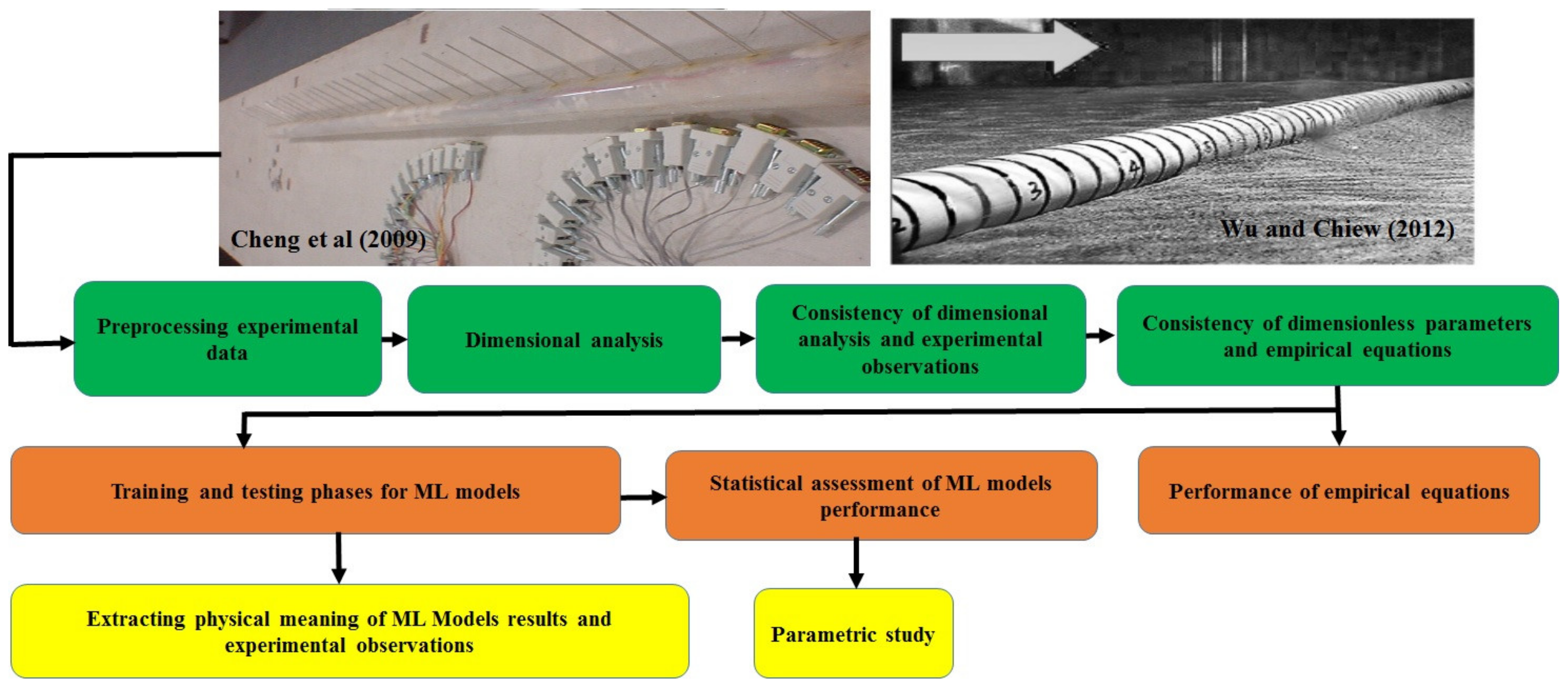
The literature review reveals that there is a lack of using ML techniques to provide physically consistent equations for the prediction of the scouring propagation rates beneath offshore pipelines subjected to currents. Therefore, the outline of this study is articulated in the following way: (i) experimental variables for feeding ML models are provided; (ii) ML models are implemented while controlling the setting parameters of each ML model; (iii) the ML models drive empirical equations; (iv) statistical analyses is performed to evaluate the empirical equations given by ML models; and (v) the physical consistency of ML models’ performance with experimental observations is controlled. A general overview of the organization of this study is outlined in Figure 1.
2. Overview of Databases
2.1. Dimensional Analysis
Based on the experimental studies from the literature, it appears that the approach flow intensity, the geometry of the offshore pipeline, the bed sediment mobility, and the physical properties of seabed sediments play a key role in scouring rate of propagation due to currents [6,7,8]. Specifically, the following function, (), which implies a relationship between the three-dimensional scour process and the governing variables, is assumed to be
where VL is the scour rate along the pipeline, is the flow shear velocity at the seabed, e is the embedment depth, D is the pipeline diameter, UC is the flow velocity due to the current, d50 is the median sediment size, is the angle of repose for the bed sediment, α is the flow incident angle to the pipeline, ρ is the mass density of water, is the mass density of bed sediment, μ is the dynamic viscosity of water, and g is the acceleration due to gravity [6,7,8].
As mentioned in Cheng et al. [6] and Wu and Chiew [7,8], the analysis of scouring rates should be carried out considering effective dimensionless parameters. Furthermore, they investigated the physical consistency of their approaches using the experimental observations to corroborate the control of the selected variables on the scouring rate of propagation. These analyses were performed with dimensionless variables, ameliorating the scale effects related to the regression-based equations from laboratory observations. In terms of the application of ML models, the use of non-dimensional parameters in the prediction of the rate of scouring propagation could enhance the ML models’ performance compared to predictive models based on raw variables (e.g., Ehteram et al. [16]; Najafzadeh and Oliveto [17]). Therefore, the present investigation applies the π-theorem to identify a set of dimensionless parameters to be considered in ML models.
Among the raw variables in Equation (1), three variables (ρ, D, VL) were utilized as repeating variables to detect nine dimensionless parameters through the Buckingham theorem:
where the above-mentioned parameters in Equation (2) can be specified as
Before finalizing the dimensional analysis, some of the dimensionless parameters could be converted to a more attractive form, as highlighted in previous studies (Cheng et al. [6]; Wu and Chiew [8]; Najafzadeh and Oliveto [17]). The first and second parameters in Equation (3) were converted to 1–e/D and 1+sinα, respectively, in Cheng et al. [6]. According to Wu and Chiew [7], the fourth and fifth parameters in Equation (3) could be converted to ρs/ρ–1 and the pipeline Froude number (FrP), respectively. Moreover, the combination of dimensionless parameters in Equation (3) could be carried out in a way that more meaningful parameters are brought out. Therefore, the dimensionless parameters in Equation (3) were re-arranged as:
Therefore, that the functional relationship (2) can be made explicit as
where VL* is the dimensionless scouring rate propagation along the offshore pipeline, θC is the Shields parameter due to the current, and ReP is the pipeline’s Reynolds number.
2.2. Description of Experimental Data
In this study, the experimental observations were obtained from three reliable studies.
Wu and Chiew [7] performed 51 experimental investigations considering uniform sand bed sediments with d50 = 0.56 mm and geometric standard deviation (σg) of 1.4. All experimental studies were conducted in a glass-sided flume whose length, width, and depth were 19 m, 1.6 m, and 0.45 m, respectively. The sediment recess section was 1.8 m long and 0.15 m deep and was placed 14 m downstream from the flume inlet. A total of 8 PVC pipelines, with D from 22 to 116 mm, were used. All experiments were performed under clear-water conditions and organized into four classes, each of which focused on the investigation of the impact of one of the dimensionless parameters e/D, FrP, θC, and the ratio of the water depth (y) on the pipeline diameter. For each class, the selected dimensionless parameter was varied, whereas all the other dimensionless parameters remained unchanged. Scouring propagation rates were not observed in four experiments, which will therefore be excluded in the proposed modeling by ML techniques.
Cheng et al. [6] carried out 81 experiments to study the scouring propagation rates in a wave flume whose length, width, and depth were 50 m, 4 m, and 2.5 m, respectively. A concrete sandpit, 4 m long, 4 m wide, and 0.25 m deep, was constructed in the test section. A clear pipeline with a smooth surface, a diameter of 50 mm, and wall thickness of 8 mm was tested. All experiments were conducted under live-bed conditions (θC = 0.046–0.104), and the embedment depth e varied in the range from 0.1D to 0.5D. The d50 value and the relative density of sediment grains (S = ρs/ρ) were 0.37 mm and 2.7, respectively. The sediment angle of repose, , was kept constant and equal to 32°, the angle of attack α ranged from 0 to 45°, and the dynamic viscosity of water, μ, was equal to 0.001 Pa·s. Among the 81 experiments, piping processes occurred in 2 experiments, and, additionally, propagation scouring rates were not observed in 35 experiments. Therefore, 44 scouring tests were considered in the proposed modeling by ML techniques. For the sake of completeness, Cheng et al. [6] suggested the following relationship to estimate the scour propagation rate:
where K is a constant that depends on α values. Equation (8) relates to current conditions, and it is the only one available in sthe literature.
Hansen et al. [18] carried out 4 scouring experiments with d50 = 0.20 mm and S = 2.65 under clear-water conditions. They considered 2 pipeline diameters (i.e., 20 and 50 mm), and the approach flow depth, equal to 0.22 m, was kept constant during all experiments.
Ultimately, 95 experimental observations were obtained from Wu and Chiew [7] (47 datasets), Cheng et al. [6] (44 datasets), and Hansen et al. [18] (4 datasets), which have been considered to develop predictive models of the scour propagation rate in current conditions. Table 1 provides the statistical characterization of the variables from the above-mentioned datasets. To perform training and testing stages for the ML techniques, 75% (71 datasets) and 25% (24 datasets) were selected randomly, respectively. As seen in Table 1, the range of the Reynolds number ReP is indicative of fully-turbulent flows, and this would imply that the effect of ReP on the prediction of VL* is negligible.
Histograms for all the dimensionless parameters are illustrated in Figure 2a–e. These histograms show the frequency distributions for the explored (independent) parameters governing scouring processes, presenting succinct and beneficial details of the experimental datasets. Incidentally, the analysis of these histogram analyses could help researchers in selecting unexplored ranges of investigation.
In Figure 2a, the α parameter had a rather fragmented distribution of the frequency, with the highest fraction of the relative frequency (70%) for sinα = 0. As depicted in Figure 2b, although the distribution of the e/D parameter is fully fragmented, the pattern of the distribution is not symmetrical. Just 2 experiments were performed with e/D = 0.286, whereas about 50% of the experimental observations were carried out with e/D = 0.143. Moreover, Figure 2c shows that the approach flow Froude number, FrP, was not deeply explored according to a high uniform distribution, and the end tail of the histogram reaches a value of FrP equal to 0.636. Figure 2d,e also shows that, in the case of the Shields parameter (θC) and the dimensionless scouring propagation rate (VL*), the distributions of the values are not symmetrical with maximum values for the relative frequencies around 50% and 55%, respectively. Additionally, most of the scouring tests were characterized by values of θC and FrP approximately equal to 0.023 and 0.40, respectively. It is essential to mention that all the scouring tests were carried out utilizing various bed sediments and both states for the approach bed sediment mobility (i.e., live-bed and clear-water conditions).
3. Implementation of ML Models
3.1. Gene-Expression Programming
GEP is known as one of the most powerful ML models; it works based on evolutionary algorithms (EAs). GEP utilizes a parse tree configuration to explore solutions, and it can provide a predictive formulation to interpret input-output systems. In addition to this, the overall formulation given by GEP includes a fair number of genetic operators [19,20]. Nevertheless, the GEP model employs a diagram of like-tree configurations with complexity, and it benefits from the merits of mathematical relationships to express a genome. The GEP model needs to assign some setting parameters, such as populations of individuals, number of generations, number of chromosomes, mutation rate, and linking functions among genes, to begin with. These factors play an important role in the goodness of the GEP performance during the training stage. GeneXproTools software was used to implement the GEP model. In the GEP performance, the validity of training and testing phases are controlled by the fitness values. In this study, root-mean-square error (RMSE) was selected as a fitness function to evaluate the GEP performance for each generation. Fitness values were scaled to 1000 by 1000/(1 + RMSE). In the GEP model, genetic operators are generally used by four strategies: optimal evolution (OE), constant fine-tuning (CFT), model fine-tuning (MFT), and sub-set selection (SSS). In this study, four alternatives of the GEP performance were considered. From the performances, the application of MFT (565.876) and OE (544.516) strategies stood at the higher goodness values in the training models in comparison with CFT (467.144) and SSS (536.205). Therefore, in the case of scouring problems below pipelines, optimal evolution methodology had promising usability; this study used the OE strategy as put forth in Najafzadeh and Oliveto [17]. The best value of the fitness function was equal to 544.516 in the training stage; the corresponding generation number obtained was 1713. Since there are four input variables for the training GEP model, the four genes can be considered the maximum number. There is no doubt that an increase in the number of genes in the structure of the GEP model causes, overall, a more complicated relationship (obtained by the GEP model). To reduce the complexity of the final equation, three genes were first considered. Then, it was found that the performance of the GEP model with three genes provided a better value of the fitness function than a GEP model developed with four genes. Table 2 indicates the setting parameters of the GEP model utilized in the optimal relationship for the prediction of the VL* parameter.
Equations (9)–(12), given by 4 alternatives (i.e., OE, SST, CFT, MFT) of the GEP model, were, respectively, obtained as follows:
3.2. Multivariate Adaptive Regression Splines
Multivariate adaptive regression splines (MARS) are a globally-recognized ML model which generates mathematical expressions by the development of linear regression [21]. The MARS model generally includes second-order spline regression. Formulas are created by the cross-validation conception that can automatically control the nonlinearities of the obtained equation and interactions among variables. To generate an equation based on spline regression, the MARS model generally makes use of a number of basis functions (BFs) with their related weighted coefficients [21]. Each BF is introduced by a variable and a knot. MARS creates an expression during two phases: the forward and the backward passes. In the forward pass, the MARS model starts with a model that consists of just the intercept/bias term, which is the mean of the output parameter values. Then, the MARS model repeatedly adds BFs in pairs to the second-order regression spline model. At each step, it detects the pair of BFs that can result in the maximum reduction value in sum-of-squares residual error. This process of adding BFs continues until the variation in residual error is too small to continue or until the maximum number of BFs is met. With regards to this research, the MARS technique approximates the scouring propagation rate through the following equation:
in which T0, Tj, BF, r, and NBF are the bias, the constant coefficients related to basis functions, the basis function, the set of dimensionless parameters, and the number of basis functions, respectively. The performance of the forward pass occasionally generates an over-fitted model. To generate an expression with more efficient generalization potential, the backward pass is performed to prune the initially-extended MARS expression. This process deletes terms one by one, eliminating the lowest effective term at each stage until it obtains the best sub-model. The performance of model subsets is evaluated using the generalized cross-validation (GCV) criterion discussed in the literature [21].
In the present research, the MARS technique was run by a computer code written in MATLAB software. The MARS model was primitively created by 10 BFs and 23.5 effective parameters. To reduce the complexity level of the initially developed MARS model, the analysis of GCV was performed. In addition to this, the k-fold was equal to 10 such that the MARS technique was performed 10 times. The forward and backward stages were carried out for each k-fold value; additionally, the number of basis functions in the final MARS model and the total effective number of parameters were obtained. The definition of the 10 performances of the MARS model is provided in Table 3, in which the results during the forward and backward stages are shown. Hence, 15 BFs were obtained to predict the scour propagation rate below offshore pipelines
in which the BF1 to BF15 formulations are presented in Table 3. All four input parameters (FrP, θC, e/D, 1+sinα) had contributions in driving Equation (14) to estimate VL*, as can be inferred from Table 4. The optimal value of GCV (0.5662) reduced the probability of over-parametrization of the MARS expression. This means that the MARS expression could efficiently detect input variables that have lower importance in the prediction of the scouring propagation rate. All coefficients in Equation (14) were fitted by the particle swarm optimization (PSO) algorithm, providing MSE = 0.2252 as the best results.
3.3. Evulotionary Polynomial Regression
EPR, as a robust data-driven models (DDMs), is developed by the multi-objective genetic algorithm (MOGA) to be applied in four various ways: (i) data analysis from the input-output records, (ii) data modeling for both static and dynamic systems, (iii) symbolic expressions for mathematical models, and (iv) decision support for the model selection [22,23,24]. Overall, EPR is an integrative model that simultaneously recruits the efficacy of MOGA with numerical regression techniques for developing simple knowledge extraction of mathematical expressions [25,26].
For the prediction of the scouring propagation rate, two types of mathematical expressions, which had the ordinary structures y = bias + ∑a·X1·X2·f(X1 × X2) and y = bias + ∑a·X1·X2·f(X1)·f(X2) were used to develop the EPR model. X is the vector of the input variables, y is the approximated output, and a is the set of coefficients. In this way, the following mathematical relationships were selected:
In the above Equations (15) and (16), O0 is the bias term, m is the maximum value of the mathematical terms, Oj is a set of coefficients, f is a user-defined function, and the ES function is a range of exponents explored by the EPR model. Previous investigations demonstrated that the use of EPR expressions with natural logarithmic inner functions had more promising efficacy in predicting the scouring propagation rates below offshore pipelines exposed to regular waves compared to predictions obtained without inner function [17]. Therefore, six terms and logarithmic inner functions in Equations (15) and (16) were considered for the EPR model. The number of generations was 4800. This issue was automatically computed regarding many factors such as the number of input parameters, the kind of inner function, and the number of dataset rows. Table 5 and Table 6 indicate the ultimate EPR expressions during training stages based on Equations (15) and (16), respectively. According to Table 5, the first model (Model #1) had the least complexity in expression with four logarithmic terms, whereas the MSE value (0.582) indicated the lowest accuracy in the prediction of scouring propagation rates. Model #5 included 6 terms with 5 logarithmic terms, providing the best results (MSE = 0.341) along with the most complicated expression. It was inferred from Table 5 that an increase in the presence of the input variables in each logarithm term could increase the precision level of approximation. For instance, the first term of Model #5 included 4 input parameters (i.e., θC, 1−e/D, 1+sinα, FrP); from Model #1 to Model #5, the more complicated the mathematical expression, the higher the precision level. Based on the expressions in Table 6, Model #5 had the highest level of accuracy (MSE = 0.585) in the training phase, whereas Model #1 had the lowest accuracy with an MSE of 0.747. Similarly, the complexity of terms and the number of terms played a key role in improving the efficiency of the expression returned by Equation (16). For instance, Model #2 (see Table 6) had one term with an MSE of 0.646, whereas Model #3 yielded more accurate predictions (MSE = 0.620) with two algebraic terms. Table 6 indicates that the third to fifth expressions (Model #3 to Model #5) had the same number of algebraic terms while providing various performance levels in the prediction of scouring propagation rate due to the existing various complexity levels in each expression. Generally, the EPR expressions given in Table 5 had more complexity and a number of algebraic terms in comparison with those presented in Table 6. Then, equations returned by EPR (based on Equation (15)) had more promising results than equations given in Table 6.
3.4. M5 Model Tree
M5MT, as a newly-established system, is generally used to learn models that estimate values. Similar to ML techniques based on the classification concepts, such as MARS and classification and regression tree (CART) models, M5 is capable of creating tree-based expressions; these regression trees provide real values at their leaves. The trees given by M5 can provide multivariate linear expressions. The M5 version of MT efficiently solves problems with high dimensionality. Compared with MARS and CART, M5MT can interpret nonlinear systems with faster executive time performance. The main merit of M5MT over the CART model is that trees have a smaller size (in terms of leaves and nodes) and a higher level of precision in the multi-task systems [27]. In M5MT, tree-like structures are provided by the divide-and-conquer technique. M5 splits the search space of data points into several subdivisions. Then, multilinear regression models are fitted on data points in each subdivision. M5MT is implemented based on several steps such as tree structure construction, error estimation, linear modeling, linear model simplification, pruning, and smoothing [27,28,29].
In this study, Weka3.9 software was utilized to develop M5MT for estimating VL* values around offshore pipelines. The following multilinear regression model is generally utilized in developing M5MT:
in which a0 is the bias term, and a1 to a4 are weighting coefficients that are computed by the least-square technique.
This research used four alternatives of M5MT based on the usability of the pruning and smoothing stages in a way that if the pruning (or smoothing) stage is considered, its state is “True” (T); otherwise, it is called “False” (F). The impacts of pruning and smoothing stages on the performance of M5MT were conceptually evaluated by RMSE values during the training and testing stages. The first alternative, M5MT#1, is related to using the pruned (T) and smoothed (T) M5MT with four rules, as seen in Table 7. The Shields parameter was adjusted as a sole splitting parameter for constructing four rules. Table 7 indicates that all the input parameters were used to provide multilinear regression equations related to their rules. Table 7 demonstrates the results of M5MT for the unpruned (F) and smoothed (T) phases. Similar to Table 7, the performance of M5MT#2 yielded four rules (see Table 8), and, consequently, four multilinear regression relationships. As demonstrated in Table 8, the first rule provided only a bias term (0.0512), and additionally, FrP was incorporated to model a linear equation for the second rule. In the case of unpruned (F) and smoothed (T) M5MT, a list of rules and relevant multilinear regression equations M5MT#3 were provided in Table 9. As seen in Table 10, all the input parameters were incorporated into 29 driving regression equations and search spaces. Regarding unpruned (F) and unsmoothed (F) M5MT, 29 rules were obtained, and M5MT#4 consequently provided 29 bias terms without incorporating the input parameters. Details of M5MT#4 performance are given in Table 11.
Generally, once M5MT was performed with ignorance of the pruning stage, the size of the tree structure increased. Although this issue can occasionally improve the accuracy level of predictions, overfitting can be imminent. For instance, in the performance of M5MT#3, the pruning phase was excluded during the training stage, resulting in an RMSE = 0.846 for the training stage and 0.554 for the testing stage. Additionally, in M5MT#4, simultaneous exclusion of pruning and smoothing stages caused the overfitting and high growth of the model tree. RMSE values for training and testing stages were equal to 0.846 and 0.554, respectively. M5MT#1 provided better predictions of the scouring propagation rate with an RMSE = 0.547 and 0.599 for training and testing, respectively, when compared with M5MT#2 (RMSE = 0.6886 and 0.713). It is practically permissible for complicated system analysis to select a typical alternative of M5MT in the presence of pruning and smoothing phases. In this way, M5MT#1 was selected as the superior model to estimate VL* in this study.
4. Discussion
4.1. Statistical Measures
To measure the efficacy of ML models’ performance for both the training and testing stages in relation with the estimation of scouring propagation rates around offshore pipelines, the index of agreement (IOA), RMSE, mean absolute error (MAE), and scatter index (SI) have been utilized. These statistical measures are defined as:
where , , , and N are the observed, predicted, and average values of , respectively, and N is the number of experimental works. The most ideal value of IOA is equal to 1, whereas the worst one is zero. In addition, the RMSE, MAE, and SI values are introduced as error functions, varying from 0 to +∞.
4.2. Statistical Performance of ML Models
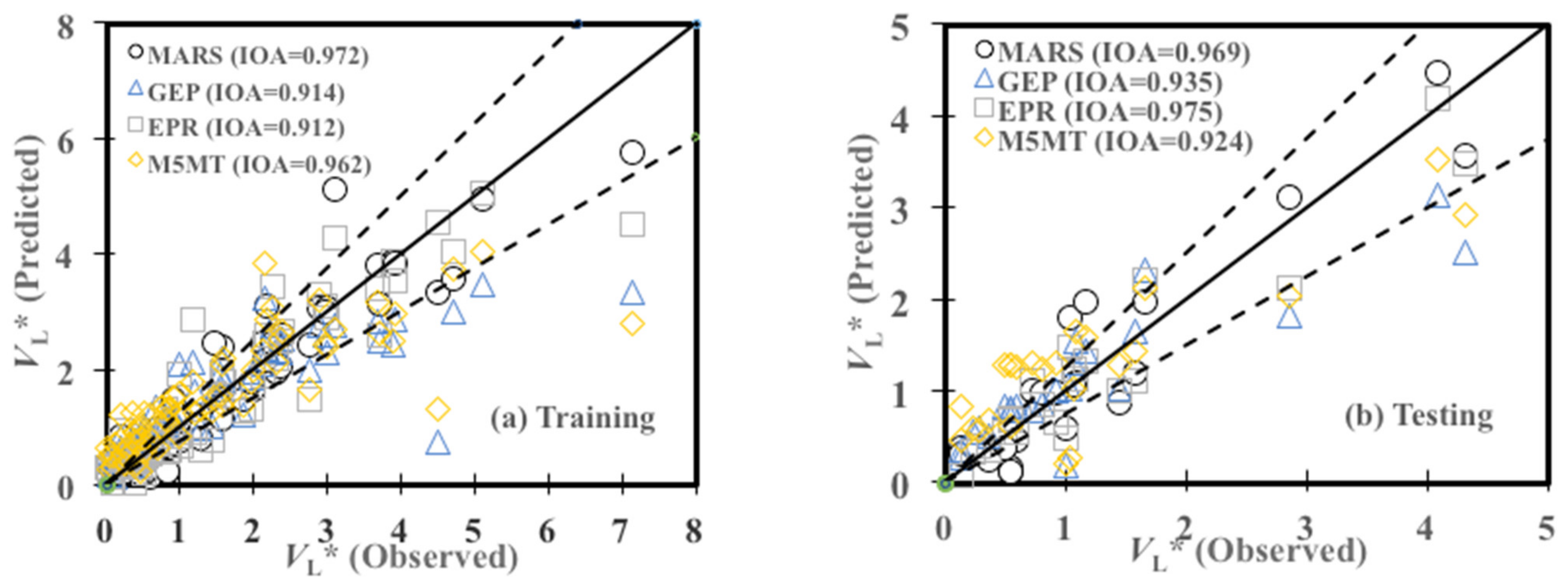
Table 12 demonstrates the performance of ML models in the estimation of scouring propagation rates (VL*) in training (calibration) and testing (validation) stages. In the training stage, as seen in Table 12, the MARS expression (Equation (14)) with an RSME of 0.474 and MAE of 1.619 gave the most promising outperformance, followed by EPR (RMSE = 0.557 and MAE = 2.754), GEP (RSME = 0.836 and MAE = 3.514), and M5MT (RSME = 0.847 and MAE = 5.347). Additionally, values of IOA and SI proved the superiority of the MARS model (IOA = 0.972 and SI = 0.322) over the EPR (IOA = 0.912 and SI = 0.378), GEP (IOA = 0.914 and SI = 0.567), and M5MT (IOA = 0.962 and SI = 0.574) techniques. According to IOA, RMSE, and SI, the models GEP and M5MT provided rather the same performance in the prediction of VL* for the training stage. Statistical measures of testing stages indicated that EPR (see Table 5 and Model#5) provided the most successful level of performance (RMSE = 0.342 and MAE = 0.300) compared to MARS (RMSE = 0.379 and MAE = 0.449), GEP (RMSE = 0.556 and MAE = 0.490), and M5MT (RMSE = 0.599 and MAE = 0.922). Additionally, values of IOA and SI indicated that EPR expression with the natural logarithmic inner function had the most remarkable potential of estimating VL* in comparison with MARS (IOA = 0.969 and SI = 0.330), GEP (IOA = 0.935 and SI = 0.483), and M5MT (IOA = 0.924 and SI = 0.507).
Figure 3 illustrates the qualitative performance of ML techniques for both the training and testing phases. Almost all data points of the training stage in Figure 3 were concentrated on the ±25% range of acceptable error. M5MT and GEP techniques significantly indicated the underestimation of VL* for the observed values of 4.5 and 7, whereas moderate overestimation has been attained by MARS and GEP techniques. Additionally, the scattering of testing data points in Figure 3b illustrated that M5MT and GEP techniques yielded moderate underpredictions and overpredictions for an observed VL* less than 2, whereas, for VL* = 2.5–5, almost all data points given by M5MT and GEP indicated underpredictions in comparison with EPR and MARS models.
4.3. Comparisons between ML Models and Related Works Regarding Complexity
In the present part of the investigation, the results of the ML models have been compared with those obtained by previous investigations considering various issues of ML models, such as the complexity of the general structure, the accuracy level, and the typical usability of optimization models in improving ML models’ performance. In the case of the convolutional structure of the ML models, EPR expression (see Table 5 and Model #5) had a more complex mathematical structure, including six algebraic terms and natural logarithmic inner function, compared with MARS expression (Equation (14)) and multilinear regression equations by M5MT. Applying the present setting parameters in the development of the EPR model along with MOGA performance was more successful in increasing the accuracy level of the VL* prediction than M5MT, with its simpler expressions and low executive time performance. Furthermore, Equation (14), given by MARS, included 15 sets of second-order polynomials along with the performance of 10 forward and backward stages, providing more complex expressions and higher executive time performance than the multilinear mathematical expressions developed by M5MT (see Table 7). In this case, the MARS expression had a promising application compared to all four alternatives of the M5MT models (including bias terms and linear expressions). In the GEP model, three typical inner functions (i.e., Tanh, Exp, Atan) with three algebraic terms could not lead to higher complex mathematical expressions than EPR expressions.
Since there is no related research work that has studied the application of ML models in the estimation of scouring propagation rates due to currents, the present results were only compared with previous investigations in terms of ML models’ complexity. All the related works were tested on the scouring propagation data due to regular waves and live-bed sediment conditions. Najafzadeh and Saberi-Movahed [15] utilized the GEP model in the structure of the GMDH model to promisingly predict the scouring propagation rates around offshore pipelines due to waves in comparison with GMDH and GEP techniques. One of the main findings of the present study is that it is consistent with the results obtained by Najafzadeh and Saberi-Movahed [15]. Moreover, an increase in the complexity of ML models causes an increase in the precision level of GMDH (or other ML models such as EPR and GEP models). For instance, Table 5 indicates that adding logarithmic terms to the EPR expression led to more accurate results, increasing performance from Model #1 with a MSE = 0.582 to Model #5 with a MSE = 0.341. In another related research work, Ehteram et al. [16] used three optimization algorithms (i.e., CBA, WA, and PSO) to improve an ANN structure for the estimation of the scouring propagation rates. All three ANN models were less complex than the EPR expression obtainedby the present study (see Table 5), and additionally, the ANN models were modeled only for wave conditions that were different from the present study. The results of this study showed that EPR, with its high degree of complexity, provided more accurate results than ANN-CBO (MAE = 0.721), ANN-WA (MAE = 0.745) and ANN-PSO (MAE = 0.814). Nevertheless, these ANN models have generally faster performance in predicting the scouring propagation rates, but the potential of MOGA in the selection of algebraic terms and exponents of variables (interactions among variables) would increase the accuracy level of ML models in this case. In Najafzadeh and Oliveto’s [17] research, EPR expressions developed by the natural logarithmic inner function provided higher complexity and accuracy than the GEP model.
4.4. Effects of the Pipeline Embedment Depth
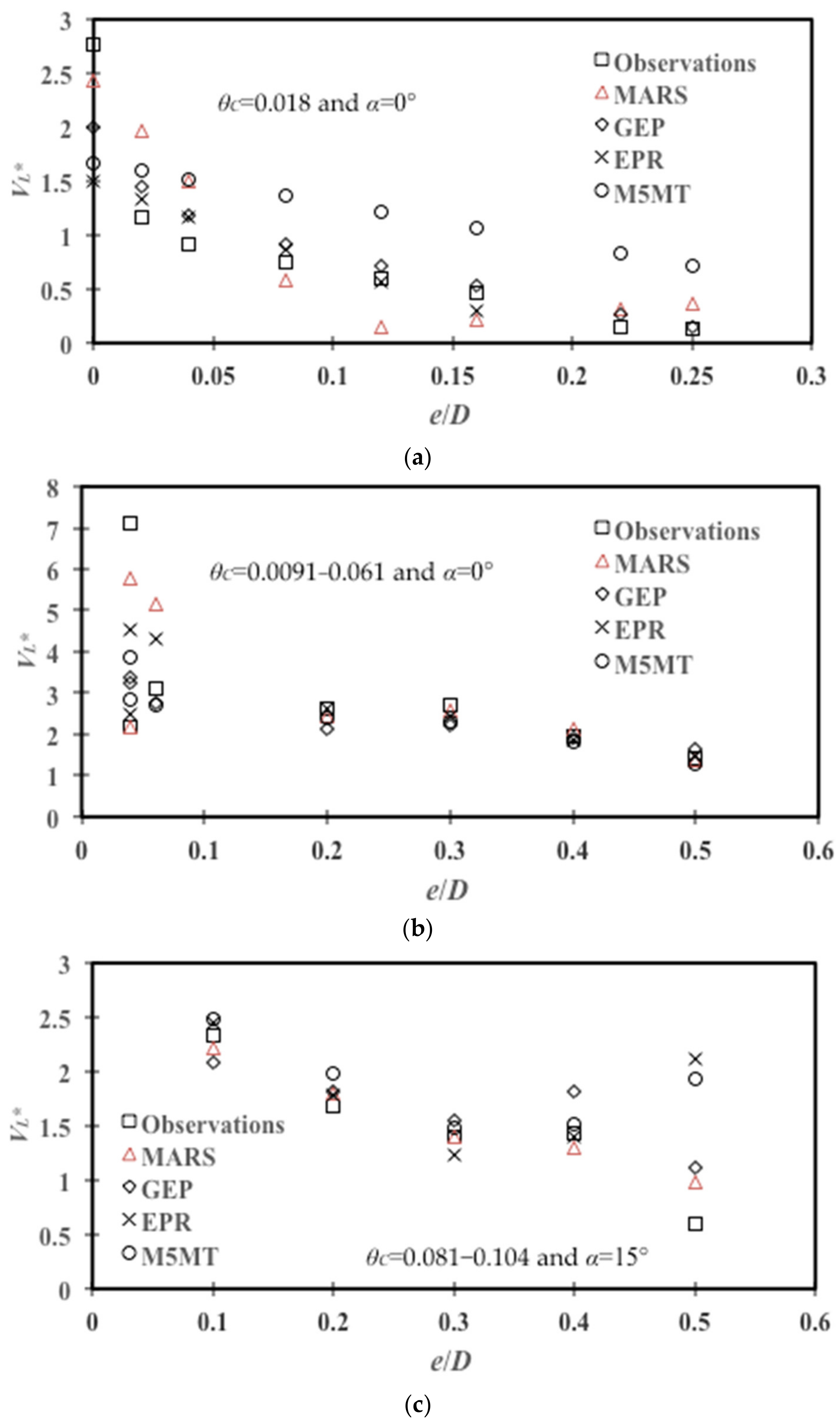
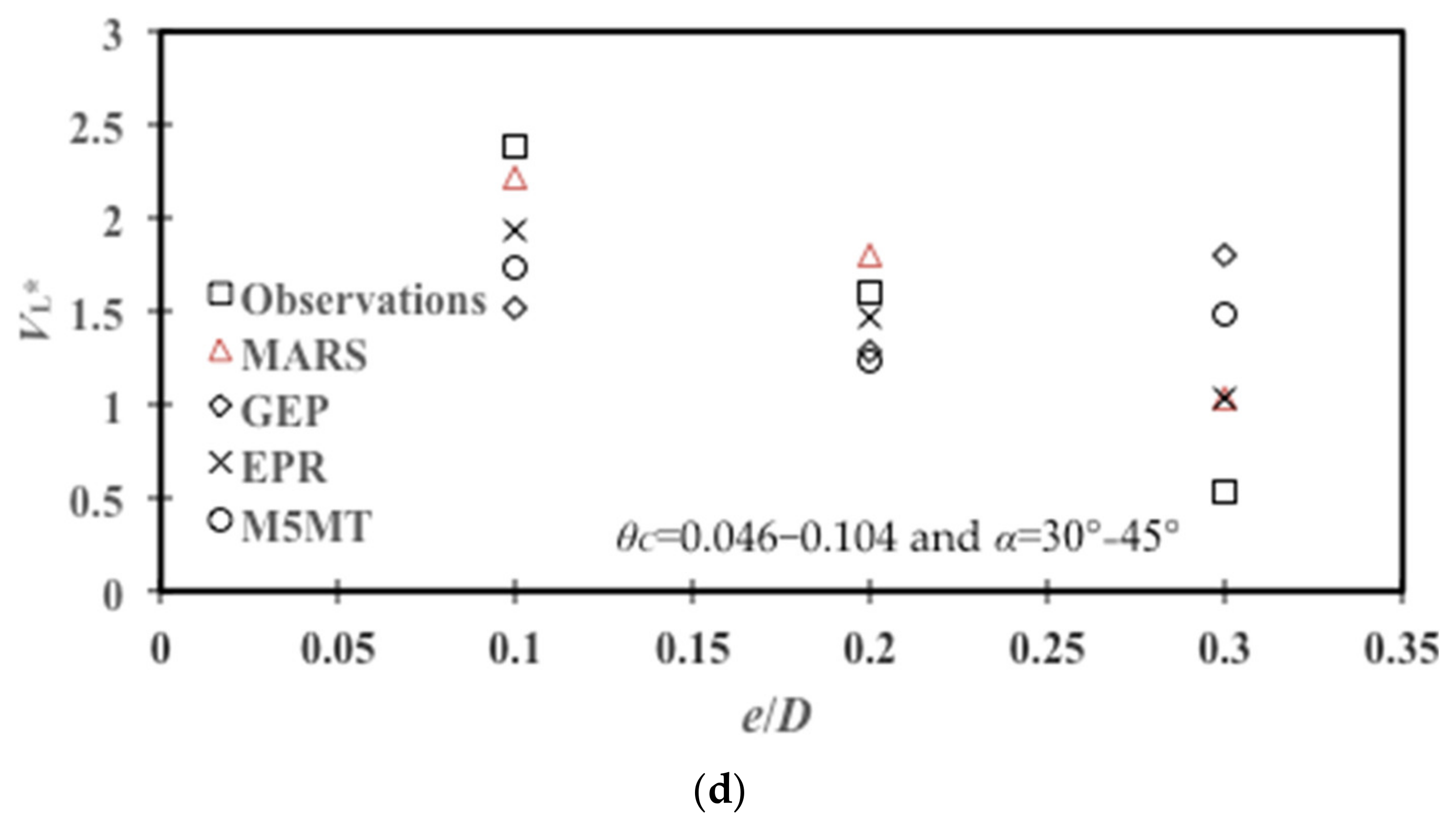
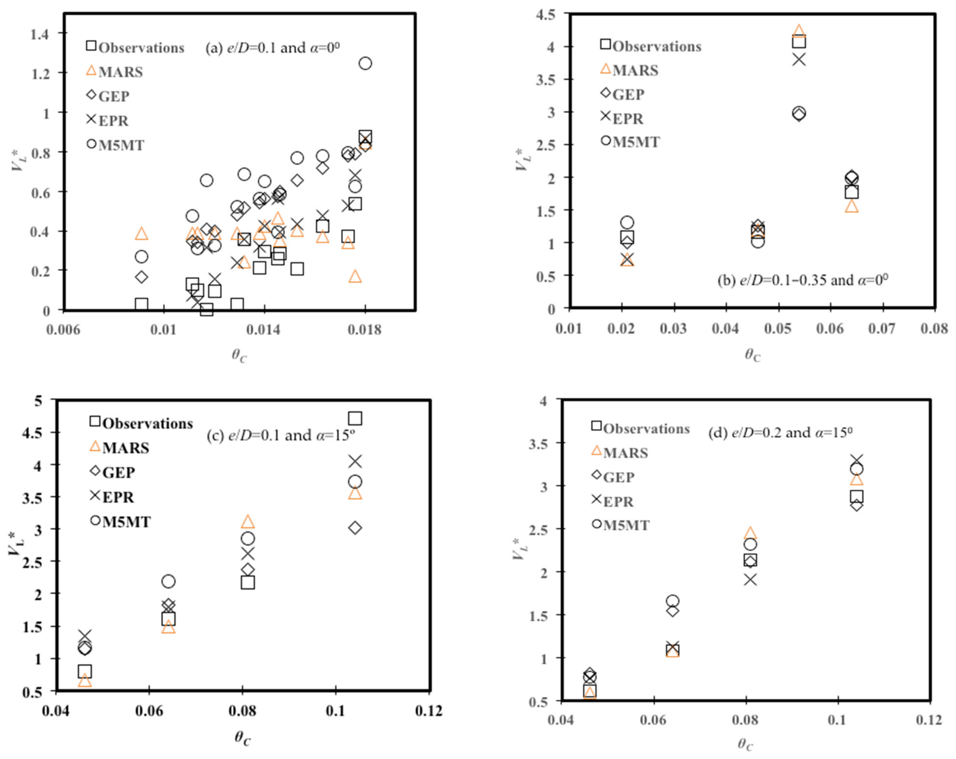
The variation of VL* values versus e/D ratios is illustrated in Figure 4. These physical behaviors were studied in four levels of θC and α values, as seen in Figure 4a–d. For θC = 0.018 and α = 0°, Figure 4a indicates that an increase in e/D value leads to a decrease in VL*. All the ML models follow the decreasing trend, consistent with observed values. For instance, MARS demonstrated that VL* declined from 1.970 in e/D = 0.02 to 0.577 in e/D = 0.08. Additionally, for the state of θC = 0.0091–0.061 and α = 0°, Figure 4b illustrated a downward trend between VL* values and e/D ratios. In Figure 4c, the variation of VL* values versus e/D ratios was provided in different viewpoints. Generally, experimental observations depicted a downward trend from VL* = 2.453 in e/D = 0.1 to VL* = 1.398 in e/D = 0.3. Afterward, VL* variations remained rather constant in e/D = 0.4, then had a decreasing trend up to e/D = 0.5. Figure 4c illustrated that all ML models follow the physical behavior of VL* versus e/D given by experimental observations for e/D = 0.1–0.4, whereas the M5MT and EPR models could not follow the downward variation of VL* values between e/D = 0.4–0.5, indicating relatively significant overpredictions. Similar to that shown in Figure 4c, MARS and EPR expressions could successfully simulate physical behaviors of VL* versus e/D values in e/D = 0.1–0.2. As seen in Figure 4d, the M5MT and MARS models have gone through upward trends at e/D = 0.3, illustrating overpredictions. The quantitative results of ML models for different ranges of θC and α parameters are presented in Table 13. As seen in Table 13, the MARS technique provided the most promising performance (RMSE = 0.197 for θC = 0.081–0.104 and α = 15°) for all ranges, except θC = 0.018 and α = 0°, whereas M5MT indicated the lowest accuracy in the prediction of VL* for all ranges, except θC = 0.046–0.104 and α = 30–45°, in which GEP expression had the worst performance.
4.5. Effects of the Shields Parameter
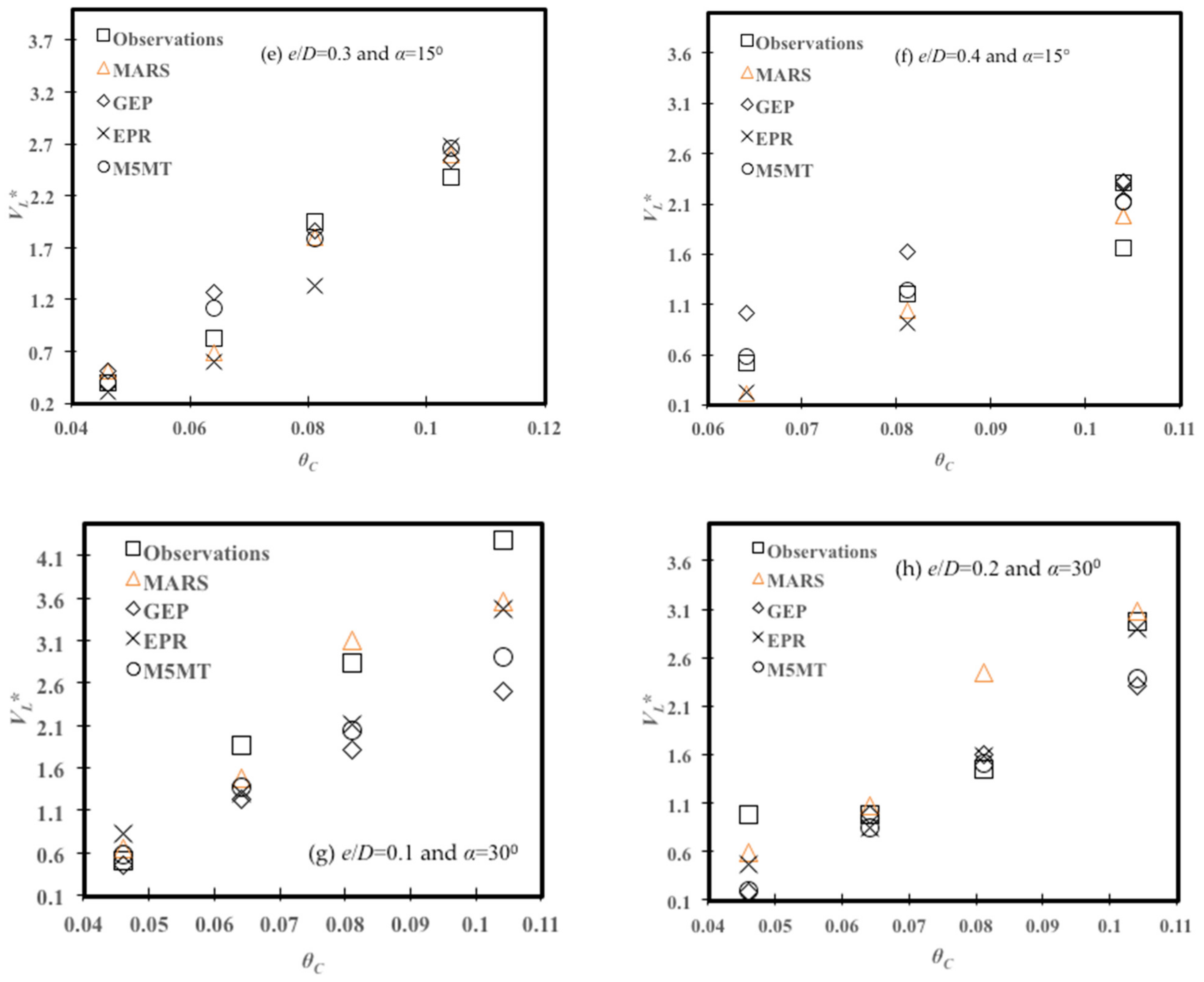
Figure 5 demonstrates the variation of VL* values versus the Shields parameter θC. As seen in Figure 5a, all ML models provided overall increasing trends for e/D = 0.1 and α = 0°. In the case of e/D = 0.01–0.035 and α = 0°, Figure 5b shows that all ML models detect physical behaviors of VL* versus θC parameter in an upward way for θC = 0.021–0.054; then, VL* decreases in θC = 0.064. Additionally, the M5MT and GEP models produced remarkable underpredictions for θC = 0.054. Figure 5c depicts the variation of VL* values versus θC for e/D = 0.1 and α = 15°. The results of the ML models indicated that the present variation had an increasing trend. As seen in Figure 5c, for θC = 0.104, ML models exhibit a certain underprediction. Similar to Figure 5c, Figure 5d–f show an increasing trend for e/D = 0.2–0.4 and α = 15°. From Figure 5g,h, for e/D = 0.1–0.2 and α = 30°, ML models generally provided an increasing trend for the variation of VL* versus the θC parameter. For θC = 0.104, all ML models underpredicted VL* for e/D = 0.1 and α = 30° (see Figure 5g) whereas GEP and M5MT had underpredictions of VL* for e/D = 0.2 and α = 30° in Figure 5h. Overall, the predicted values of VL* given by ML models were in good agreement with experimental observations. To allow quantitative comparisons of the ML models’ performance in the four ranges of e/D and α, the results of the RMSE are presented in Table 13. Table 13 indicates that EPR expression had the most successful performance for e/D = 0.1 and α = 0° with an RMSE of 0.185, e/D = 0.1 and α = 15° with an RMSE of 0.490, and e/D = 0.1 and α = 30° with an RMSE of 0.278. Additionally, the MARS model had the best results for ranges e/D = 0.1–0.35 and α = 0° (RMSE = 0.183), e/D = 0.2 and α = 15° (RMSE = 0.191), e/D = 0.3 and α = 15° (RMSE = 0.165), e/D = 0.2 and α = 30° (RMSE = 0.439). Moreover, Table 13 shows that GEP had the worst performance for e/D = 0.2 and α = 30° (RMSE = 1.075), as well as in case of e/D = 0.1 and α = 15°, in which the GEP model still had the lowest level of accuracy (RMSE = 0.880).
4.6. Effects of the Approach Flow Froude Number
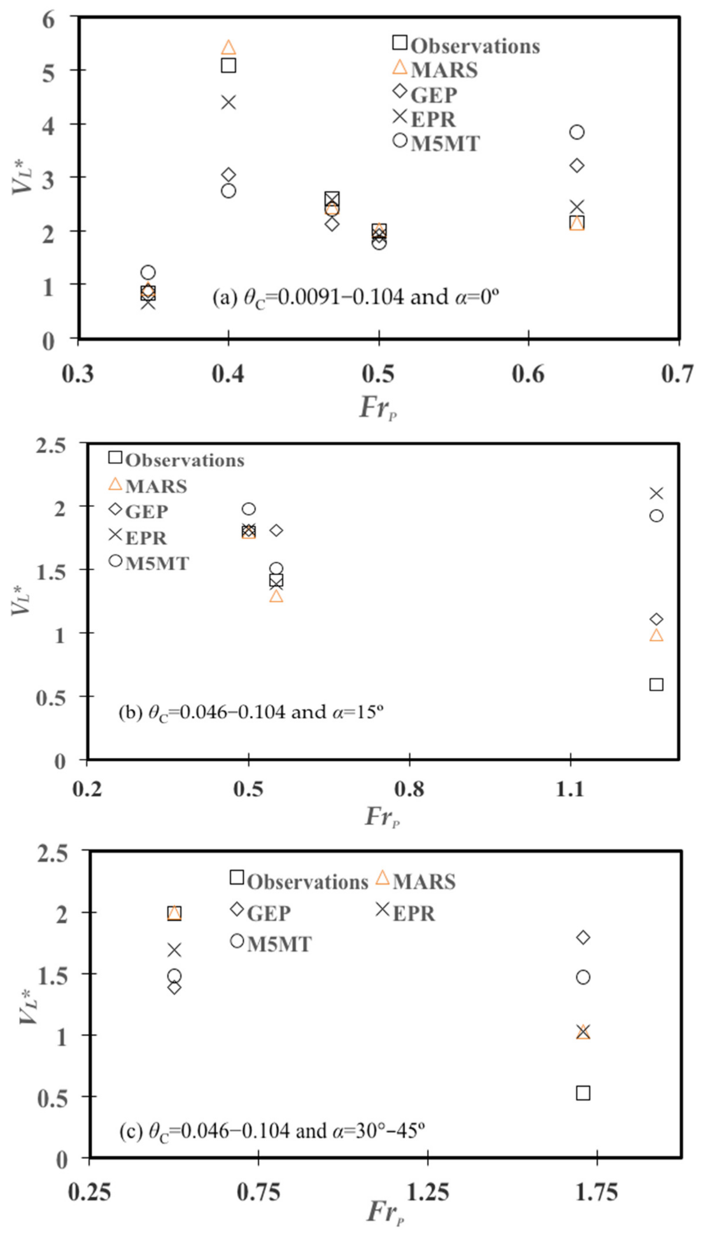
Figure 6 shows the variations of VL* versus FrP for three ranges of θC and α. From Figure 6a, the performance of the ML models was in good agreement with experimental observations for FrP = 0.34, 0.47, and 0.5. Overall, the qualitative results of ML models indicated that VL* variations had an increasing trend for FrP = 0.346–0.4; then, a downward trend was obtained for FrP = 0.4–0.5. Besides, values of VL* given by the ML techniques increased at FrP = 0.63. As seen in Figure 6a, all the ML models, except MARS expression, had relatively remarkable underprediction for FrP = 0.4, whereas M5MT and GEP techniques overpredicted VL* values at FrP = 0.63. In Figure 6b, experimental observations indicated that the variation of VL* values had a declining trend for FrP = 0.5–1.26, whereas EPR and M5MT techniques overpredicted significantly compared to GEP and MARS expressions. As illustrated in Figure 6c, MARS and EPR models indicated a downward trend for FrP = 0.5–1.71, whereas GEP and M5MT overpredicted significantly. In regard to the quantitative performance of ML models, the MARS model had the most successful evaluation in the prediction of VL* for all ranges θC = 0.0091–0.1045 and α = 0° (RMSE = 0.173), θC = 0.046–0.104 and α = 15° (RMSE = 0.235), and θC = 0.046–0.104 and α = 30–45° (RMSE = 0.359). In contrast, M5MT, EPR, and GEP yielded the lowest level of accuracy in θC = 0.0091–0.1045 and α = 0° (RMSE = 1.315), θC = 0.046–0.104 and α = 15° (RMSE = 0.872), and θC = 0.046–0.104 and α = 30–45° (RMSE = 0.993), respectively (Table 13).
5. Conclusions
In the present research, various ML models based on evolutionary computing and classification concepts have been utilized to predict the scouring propagation rate around offshore pipelines exposed to currents. Effective dimensionless parameters (i.e., 1 – e/D, 1 + sinα, θC, FrP) obtained from dimensional analysis of the scouring tests were directly incorporated into the presented equations through the performance of ML models. The main findings of this research can be summarized as follows.
ML models provided explicit formulas with promising performance for the estimation of the scouring propagation rate. EPR expression included a mathematical structure with the highest degree of nonlinearity, followed by Equation (14) (given by the second-order polynomial MARS model) and the multilinear regression equation by M5MT. In the GEP model, a kind of inner function played a key role in increasing the precision level of performance (Equation (9)) through an optimal evolutionary technique. The predictive equations resulting from the ML models are somewhat complex and have several fitting parameters, which are not so numerous when taking into account the geometrical and hydraulic conditions (even including live-bed and clear-water approaching flows) considered in this study. However, these equations have the considerable advantage of fitting the experimental data with performances that are significantly higher than the currently available literature formulas. Their structure is somewhat complex and inhibits an immediate identification of the role performed by each governing parameter (though a sensitivity analysis could be a replacement in this regard), but they could be easily implemented in numerical codes. Moreover, according to Table 1, their ranges of application are: 0 ≤ e/D ≤ 0.5, 0° ≤ α ≤ 45°, 0.22 ≤ FrP ≤ 0.63, and 0.01 ≤ θC ≤ 0.10.
The ML models considered in this study definitely perform better than the current empirical models. However, their performance differs from one model to another depending on the structure/algorithm of the model itself. This study also remarks on these differences (highlighting which model would perform better) in a physical context characterized by a limited number of data (95 experimental observations) despite the complexity of the phenomena. Statistical measures of ML models indicated that MARS could yield 15 BFs (including linear and polynomial equations) and the best performance in the training states whereas, for the testing stage, EPR expression with natural logarithmic functions resulted in the most level of precision for the prediction of VL*.
Quantitative and qualitative representations for variations of VL* values versus e/D were provided to obtain physical behaviors with variations in θC and α values. Generally, MARS and GEP expressions simulated well the variations of VL* values versus e/D ratios through a downward trend compared to EPR and M5MT techniques. These downward variations were in good agreement with experimental variations for different levels of θC and α (for instance, θC = 0.018 and α = 0°; θC = 0.0091–0.061 and α = 0°).
A parametric study of VL* variations versus θC values was carried out in various levels of e/D and α. All ML models provided increasing trends for levels of e/D and α. Generally, predictions of scouring propagation rates (given by ML models) were in good harmony with experiments by Hansen et al. [18], Cheng et al. [6], and Wu and Chiew [7].
Driving physical variations of VL* values versus the pipeline Froude number (FrP) values were conceptualized for three levels of θC and α values. Although MARS and EPR expressions demonstrated a downward trend for some values of FrP, the performance of the ML models generally could follow decreasing trends for θC = 0.0091–0.104 and α = 0°, θC = 0.046–0.104 and α = 15°, and θC = 0.046–0.104 and α = 30–45°, probably due to live-bed conditions.
ML model-performed equations exhibited physical consistency with experimental investigations, so they could result in reliable estimations of scouring propagation rates, which are utilized to consider the practical design of offshore pipelines while focusing on preventative measures of erosion and scouring. The analysis of data was carried out considering dimensionless governing parameters of great impact in sediment transport phenomena (e.g., the pipeline Froude number and the Shields parameter). This approach allows the extension of the proposed predictive equations to the field because the experimental data used in this study would appear free from scale effects. However, more experimental observations would be useful and desirable, especially those looking at the unexplored ranges highlighted in the histograms in Figure 2. The combined action of current and waves would need more attention, as would the collection of field data, which are not currently available to the authors’ knowledge.
Author Contributions
Conceptualization, M.N. and G.O.; methodology, M.N.; software, M.N.; validation, M.N. and G.O.; formal analysis, M.N. and G.O.; investigation, M.N. and G.O.; data curation, M.N. and G.O.; writing—original draft preparation, M.N. and G.O.; writing—review and editing, M.N. and G.O.; visualization, M.N. and G.O.; supervision, M.N. and G.O. All authors have read and agreed to the published version of the manuscript.
Funding
This research received no external funding.
Institutional Review Board Statement
Not applicable.
Informed Consent Statement
Not applicable.
Data Availability Statement
Not applicable.
Acknowledgments
This research has been supported by Graduate University of Advanced Technology (Kerman-Iran) under grant number of 2594.
Conflicts of Interest
The authors declare no conflict of interest.
References
- Bai, Y.; Bai, Q. Subsea Engineering Handbook; Gulf Professional Publishing: Burlington, MA, USA, 2010. [Google Scholar]
- Barrette, P. Offshore pipeline protection against seabed gouging by ice: An overview. Cold Reg. Sci. Technol. 2011, 69, 3–20. [Google Scholar] [CrossRef]
- Palmer, A.C.; Been, K. Pipeline geohazards for Arctic conditions. In Deepwater Foundations and Pipeline Geomechanics; McCarron, W.O., Ed.; J. Ross Publishing: Fort Lauderdale, FL, USA, 2011; pp. 171–178. [Google Scholar]
- Palmer, A.C.; King, R.A. Subsea Pipeline Engineering, 2nd ed.; PennWell Corporation: Tulsa, OK, USA, 2008. [Google Scholar]
- Ramakrishnan, T.V. Offshore Engineering; Gene-Tech Books: New Delhi, India, 2008. [Google Scholar]
- Cheng, L.; Yeow, K.; Zhang, Z.; Teng, B. Three-dimensional scour below offshore pipelines in steady currents. Coast. Eng. 2009, 56, 577–590. [Google Scholar] [CrossRef]
- Wu, Y.; Chiew, Y.-M. Three-dimensional scour at submarine pipelines. J. Hydraul. Eng. ASCE 2012, 138, 788–795. [Google Scholar] [CrossRef]
- Wu, Y.; Chiew, Y.-M. Mechanics of three-dimensional pipeline scour in unidirectional steady current. J. Pipeline Syst. Eng. 2013, 4, 3–10. [Google Scholar] [CrossRef]
- Cheng, L.; Yeow, K.; Zang, Z.; Li, F. 3D scour below pipelines under waves and combined waves and currents. Coast. Eng. 2014, 83, 137–149. [Google Scholar] [CrossRef] [Green Version]
- Fredsøe, J.; Sumer, B.M.; Arnskov, M.M. Time scale for wave/current scour below pipelines. Int. J. Offshore Polar Eng. 1992, 2, 13–17. [Google Scholar]
- Sumer, B.M.; Fredsøe, J. Scour around pipelines in combined waves and current. In Proceedings of the 15th Conference on Offshore Mechanics and Arctic Engineering (OMAE), Florence, Italy, 16–20 June 1996. [Google Scholar]
- Sumer, B.M.; Truelsen, C.; Sichmann, T.; Fredsøe, J. Onset of scour below pipelines and self-burial. Coast. Eng. 2001, 42, 313–335. [Google Scholar] [CrossRef]
- Arya, A.K.; Shingan, B. Scour-mechanism, detection and mitigation for subsea pipeline integrity. Int. J. Eng. Technol. 2012, 1, 1–14. [Google Scholar]
- Zhang, B.; Gong, R.; Wang, T.; Wang, Z. Causes and treatment measures of submarine pipeline free-spanning. J. Mar. Sci. Eng. 2020, 8, 329. [Google Scholar] [CrossRef]
- Najafzadeh, M.; Saberi-Movahed, F. GMDH-GEP to predict free span expansion rates below pipelines under waves. Mar. Georesour. Geotec. 2019, 37, 375–392. [Google Scholar] [CrossRef]
- Ehteram, M.; Ahmed, A.N.; Ling, L.; Fai, C.M.; Latif, S.D.; Afan, H.A.; Banadkooki, F.B.; El-Shafie, A. Pipeline scour rates prediction-based model utilizing a Multilayer Perceptron-Colliding Body algorithm. Water 2020, 12, 902. [Google Scholar] [CrossRef] [Green Version]
- Najafzadeh, M.; Oliveto, G. Exploring 3D wave-induced scouring patterns around subsea pipelines with artificial intelligence techniques. Appl. Sci. 2021, 11, 3792. [Google Scholar] [CrossRef]
- Hansen, E.A.; Staub, C.; Fredsøe, J.; Sumer, B.M. Time-development of scour induced free spans of pipelines. In Proceedings of the 10th Conference on Offshore Mechanics and Arctic Engineering (OMAE), Stavanger, Norway, 23–28 June 1991. [Google Scholar]
- Ferreira, C. Gene expression programming: A new adaptive algorithm for solving problems. Complex Syst. 2001, 13, 87–129. [Google Scholar]
- Ferreira, C. Gene Expression Programming, 2nd ed.; Springer: Berlin/Heidelberg, Germany, 2006. [Google Scholar]
- Friedman, J.H. Multivariate adaptive regression splines. Ann. Statist. 1991, 19, 1–67. [Google Scholar] [CrossRef]
- Giustolisi, O.; Savic, D.A. A symbolic data-driven technique based on evolutionary polynomial regression. J. Hydroinf. 2006, 8, 207–222. [Google Scholar] [CrossRef] [Green Version]
- Giustolisi, O.; Savic, D.A. Advances in data-driven analyses and modelling using EPR-MOGA. J. Hydroinf. 2009, 11, 225–236. [Google Scholar] [CrossRef]
- Giustolisi, O.; Doglioni, A.; Savic, D.A.; Webb, B.W. A multi-model approach to analysis of environmental analysis. Environ. Modell. Softw. 2007, 22, 674–682. [Google Scholar] [CrossRef] [Green Version]
- Savic, D.A.; Giustolisi, O.; Berardi, L.; Shepherd, W.; Djordjevic, S.; Saul, A. Modelling sewer failure by evolutionary computing. In Proceedings of the Institution of Civil Engineers-Water Management; Thomas Telford Ltd: London, UK, 2006; Volume 159, pp. 111–118. [Google Scholar] [CrossRef]
- Berardi, L.; Giustolisi, O.; Kapelan, Z.; Savic, D.A. Development of pipe deterioration models for water distribution systems using EPR. J. Hydroinf. 2008, 10, 113–126. [Google Scholar] [CrossRef] [Green Version]
- Quinlan, J.R. Learning with continuous classes. In Proceedings of the Australian Joint Conference on Artificial Intelligence (AI’92), Hobart, Australia, 16–18 November 1992. [Google Scholar]
- Mokhtia, M.; Eftekhari, M.; Saberi-Movahed, F. Dual-manifold regularized regression models for feature selection based on hesitant fuzzy correlation. Knowl Based Syst. 2021, 229, 107308. [Google Scholar] [CrossRef]
- Mokhtia, M.; Eftekhari, M.; Saberi-Movahed, F. Feature selection based on regularization of sparsity based regression models by hesitant fuzzy correlation. Appl. Soft Comput. 2020, 91, 106255. [Google Scholar] [CrossRef]
Figure 1.
Flow chart of the present research work.

Figure 2.
Frequency and cumulative relative frequency for the non-dimensional parameters considered in the present research: (a) flow attack angle α to the offshore pipeline; (b) ratio of the pipeline embedded depth to pipeline diameter, e/D; (c) approaching flow Froude number to the offshore pipeline, FrP; (d) Shields parameter due to current, θC; (e) dimensionless scouring propagation rate around offshore pipeline along the longitudinal direction, VL*.

Figure 3.
Performance of ML models for prediction of VL* in the (a) training and (b) testing stages.
Figure 3.
Performance of ML models for prediction of VL* in the (a) training and (b) testing stages.

Figure 4.
Variations of dimensionless VL* against various e/D values at (a) θC = 0.018 and α = 0°, (b) θC = 0.091–0.061 and α = 0°, (c) θC = 0.081–0.104 and α = 15°, and (d) θC = 0.046–0.104 and α = 30–45°.
Figure 4.
Variations of dimensionless VL* against various e/D values at (a) θC = 0.018 and α = 0°, (b) θC = 0.091–0.061 and α = 0°, (c) θC = 0.081–0.104 and α = 15°, and (d) θC = 0.046–0.104 and α = 30–45°.


Figure 5.
Variations of dimensionless VL* against various θC for (a) e/D = 0.1 and α = 0°, (b) e/D = 0.1–0.35 and α = 0°, (c) e/D = 0.1 and α = 15°, (d) e/D = 0.2 and α = 15°, (e) e/D = 0.3 and α = 15°, (f) e/D = 0.4 and α = 15°, (g) e/D = 0.1 and α = 30°, and (h) e/D = 0.2 and α = 30°.
Figure 5.
Variations of dimensionless VL* against various θC for (a) e/D = 0.1 and α = 0°, (b) e/D = 0.1–0.35 and α = 0°, (c) e/D = 0.1 and α = 15°, (d) e/D = 0.2 and α = 15°, (e) e/D = 0.3 and α = 15°, (f) e/D = 0.4 and α = 15°, (g) e/D = 0.1 and α = 30°, and (h) e/D = 0.2 and α = 30°.


Figure 6.
Variations of dimensionless VL* against FrP for (a) θC = 0.0091–0.1045 and α = 0°, (b) θC = 0.046–0.104 and α = 15°, and (c) θC = 0.046–0.104 and α = 30–45°.
Figure 6.
Variations of dimensionless VL* against FrP for (a) θC = 0.0091–0.1045 and α = 0°, (b) θC = 0.046–0.104 and α = 15°, and (c) θC = 0.046–0.104 and α = 30–45°.


Table 1.
Statistical characterization of variables for feeding ML techniques.
| Dimensional Variables | Minimum | Maximum | Average | Standard Deviation | Skewness |
| D (m) | 0.020 | 0.116 | 0.04425 | 0.012 | 1.538 |
| e (m) | 0.0 | 0.025 | 0.00848 | 0.00643 | 1.168 |
| d50 (m) | 0.0002 | 0.00057 | 0.00055 | 0.0000719 | −4.7055 |
| u* (m/s) | 0.0091 | 0.0314 | 0.02065 | 0.00624 | 0.2595 |
| α (degree) | 0 | 45 | 5.454 | 10.1027 | 1.8212 |
| UC (m/s) | 0.158 | 0.42 | 0.2817 | 0.07571 | 0.5154 |
| y (m) | 0.09 | 0.470 | 0.2992 | 0.156 | 0.1067 |
| VL (m/s) | 0.0000084 | 0.0056 | 0.00154 | 0.00122 | 1.2503 |
| Dimensionless Parameters | Minimum | Maximum | Average | Standard Deviation | Skewness |
| e/D | 0 | 0.5 | 0.1782 | 0.1256 | 1.224 |
| θC | 0.0091 | 0.104 | 0.04527 | 0.03221 | 0.5974 |
| FrP | 0.225 | 0.6321 | 0.4354 | 0.0927 | 0.4613 |
| ReP | 5600 | 21,000 | 14,087.02 | 3917.98 | 0.40736 |
| VL* | 0.0000481 | 5.1082 | 0.9057 | 1.277 | 1.4825 |
Table 2.
Setting parameters of the proposed structure of GEP models.
| Parameters | Description of Parameters | Setting of Parameters |
|---|---|---|
| P1 | Function set | +, −, ×, /, Power(x2), (1-x), Average(x1, x2), Tanh(x), 3Rt, Ln, Min, Max |
| P2 | Linking function | Addition |
| P3 | Mutation rate | OE (0.003), CFT (0), MFT (0), SSS (0) |
| P4 | Inversion rate | OE (0.00546), CFT (0), MFT (0), SSS (0.0082) |
| P5 | One-point and two-point recombination rates | OE (0.00277), CFT (0), MFT (0), SSS (0.0028) |
| P6 | Gene recombination rate | OE (0.00277), CFT (0), MFT (0.0129), SSS (0.0028) |
| P7 | Permutation | OE (0.00546), CFT (0), MFT (0), SSS (0.0082) |
| P8 | Maximum tree depth | OE (4), CFT (3), MFT (5), SSS (4) |
| P9 | Number of genes | 3 |
| P10 | Number of chromosomes | 30 |
| P11 | Number of generations | OE (1713), CFT (961), MFT (2700), SSS (909) |
| P12 | Best fitness value | OE (544.516), CFT (467.144), MFT (565.876), SSS (536.205) |
Table 3.
Characterizations of MARS models during the forward and backward stages.
| k-Fold | Number of BFs in the Final Model | Total Effective Number of Parameters | Executive Time (s) |
|---|---|---|---|
| 1 | 11 | 26 | 0.57 |
| 2 | 7 | 16 | 0.69 |
| 3 | 14 | 33.5 | 0.99 |
| 4 | 9 | 21 | 0.71 |
| 5 | 12 | 28.5 | 0.74 |
| 6 | 12 | 28.5 | 0.66 |
| 7 | 11 | 26 | 0.67 |
| 8 | 12 | 28.5 | 0.99 |
| 9 | 6 | 13.5 | 0.71 |
| 10 | 14 | 33.5 | 0.58 |
Table 4.
Coefficients and basis functions for MARS models in scour rate prediction.
| Basis Functions | Basis Functions | ||
|---|---|---|---|
| BF1 | max (0, 0.1−e/D) | BF9 | max (0, FrP−0.34623)·max (0, 0.3−e/D) |
| BF2 | max (0, FrP−0.34623) | BF10 | max (0, FrP−0.34623)·max (0, e/D−0.3) |
| BF3 | max (0, FrP−0.34623)·max (0, 0.046−θC) | BF11 | max (0, FrP−0.47128) |
| BF4 | max (0, θC−0.018)·max (0, 0.1−e/D) | BF12 | max (0, 0.47128−FrP)·max (0, θC−0.014) |
| BF5 | max (0, FrP−0.34623)·max (0, 0.054−θC) | BF13 | max (0, θC−0.014) |
| BF6 | max (0, 1−sinα)·max (0, θC−0.021) | BF14 | max (0, e/D−0.6) |
| BF7 | max (0, 0.1−e/D)·max (0, FrP−0.52841) | BF15 | max (0, 0.6−e/D) |
| BF8 | max (0, 0.1−e/D)·max (0, 0.52841−FrP) | BF16 | 0 |
Table 5.
Mathematical expressions developed by Equation (15) with logarithmic inner function.
| Model No. | Expression | MSE |
|---|---|---|
| Model #1 | 0.582 | |
| Model #2 | 0.460 | |
| Model #3 | 0.449 | |
| Model #4 | 0.437 | |
| Model #5 | 0.341 |
Table 6.
Mathematical expressions developed by Equation (16) with logarithmic inner function.
| Model No. | Expression | MSE |
|---|---|---|
| Model #1 | 0.747 | |
| Model #2 | 0.646 | |
| Model #3 | 0.620 | |
| Model #4 | 0.596 | |
| Model #5 | 0.585 |
Table 7.
List of M5MT#1 details in VL* estimates.
| Rules of M5MT#1 Focusing on Pruning and Smoothing Phases | |
|---|---|
| If θC ≤ 0.018: | |
| | If θC ≤ 0.013:LM1 | |
| | If θC > 0.013:LM2 | |
| If θC > 0.018 : | |
| | If θC ≤ 0.05:LM3 | |
| | If θC > 0.05:LM4 | |
| Multilinear Regression Equations | |
| LM1 | VL* = −2.0495 + 20.7493θC + 1.4622(1 − e/D) − 0.8277(1 + sinα) + 5.2496FrP |
| LM2 | VL* = −2.1368 + 16.5994θC + 1.4622(1 − e/D) − 0.8277(1 + sinα) + 5.7554FrP |
| LM3 | VL* = 0.062 + 18.2934θC + 3.8163(1 − e/D) − 2.4011(1 + sinα) − 0.3838FrP |
| LM4 | VL* = −2.0857 + 24.1656θC + 5.3836(1 − e/D) − 3.3503(1 + sinα) + 4.4672FrP |
Table 8.
List of M5MT#2 details in VL* estimates.
| Multilinear Regression Equations | |
|---|---|
| LM1 | VL* = 0.0512 |
| LM2 | VL* = −0.6047 + 2.5289FrP |
| LM3 | VL* = 0.062 + 37.1095θC + 4.4068(1 − e/D) − 2.899(1 + sinα) − 10.5248FrP |
| LM4 | VL* = −1.1712 + 45.4636θC + 7.2873(1 − e/D) − 4.6271(1 + sinα) |
Table 9.
List of driven rules of M5MT#3 in VL* estimates.
| If θC ≤ 0.018 : | If θC ≤ 0.013 : LM1 | If θC > 0.013 : | | If FrP ≤ 0.367 : LM2 | | If FrP > 0.367 : | | | If θC ≤ 0.015 : LM3 | | | If θC > 0.015 : LM4 If θC > 0.018 : | If θC ≤ 0.05 : | | If FrP ≤ 0.361 : | | | If 1 − e/D ≤ 0.89 : | | | | If 1 − e/D ≤ 0.82 : LM5 | | | | If 1 − e/D > 0.82 : LM6 | | | If 1 − e/D > 0.89 : | | | | If 1 − e/D ≤ 0.94 : LM7 | | | | If 1 − e/D > 0.94 : LM8 | | If FrP > 0.361 : | | | If 1 + sinα ≤ 1.129 : | | | | If θC ≤ 0.019 : | | | | | If FrP ≤ 0.425 : LM9 | | | | | If FrP > 0.425 : LM10 | | | | If θC > 0.019 : | | | | | If FrP ≤ 0.387 : LM11 | | | | | If FrP > 0.387 : | | | | | | If 1 − e/D < = 0.7 : LM12 | | | | | | If 1 − e/D > 0.7 : | | | | | | | If FrP ≤ 0.42 : LM13 | | | | | | | If FrP > 0.42 : LM14 | | | If 1 + sinα > 1.129 : | | | | If 1 − e/D ≤ 0.85 : LM15 | | | | If 1 − e/D > 0.85 : LM16 | If θC > 0.05 : | | If 1 + sinα ≤ 1.129 : | | | If 1 − e/D ≤ 0.75 : | | | | If θC ≤ 0.092 : | | | | | If 1 − e/D ≤ 0.65 : LM17 | | | | | If 1 − e/D > 0.65 : LM18 | | | | If θC > 0.092 : LM19 | | | If 1 − e/D > 0.75 : | | | | If 1 − e/D ≤ 0.95 : | | | | | If θC ≤ 0.073 : | | | | | | If θC ≤ 0.059 : LM20 | | | | | | If θC ≤ 0.059 : LM20 | | | | | | If θC > 0.059 : LM21 | | | | | If θC > 0.073 : LM22 | | | | If 1 − e/D > 0.95 : LM23 | | If 1 + sinα > 1.129 : | | | If θC ≤ 0.092 : | | | | If 1 − e/D ≤ 0.85 : | | | | | If θC ≤ 0.073 : LM24 | | | | | If θC > 0.073 : | | | | | | If 1 − e/D ≤ 0.75 : LM25 | | | | | | If 1 − e/D > 0.75 : LM26 | | | | If 1 − e/D > 0.85 : LM27 | | | If θC > 0.092 : | | | | If 1 − e/D ≤ 0.75 : LM28 | | | | If 1 − e/D > 0.75 : LM29 |
Table 10.
List of multilinear regression models extracted from M5MT#3 rules.
| Multilinear Regression Equations | |
|---|---|
| LM1 | VL* = −2.0495 + 20.7493θC + 1.4622(1 − e/D) − 0.8277(1 + sinα) + 5.2496FrP |
| LM2 | VL* = −2.0955 + 16.5994θC + 1.46222(1 − e/D) − 0.8277(1 + sinα) + 5.629FrP |
| LM3 | VL* = −2.0867 + 16.5994θC + 1.46222(1 − e/D) − 0.8277(1 + sinα) + 5.629FrP |
| LM4 | VL* = −2.0876 + 16.5994θC + 1.46222(1 − e/D) − 0.8277(1 + sinα) + 5.629FrP |
| LM5 | VL* = −1.5165 + 11.9305θC + 4.4349(1 − e/D) − 1.904(1 + sinα) + 1.4209FrP |
| LM6 | VL* = −1.5153 + 11.9305θC + 4.4349(1 − e/D) − 1.904(1 + sinα) + 1.4209FrP |
| LM7 | VL* = −1.3564 + 11.9305θC + 4.4349(1 − e/D) − 1.904(1 + sinα) + 1.4209FrP |
| LM8 | VL* = −1.3597 + 37.1095θC + 4.4068(1 − e/D) − 1.904(1 + sinα) + 1.4209FrP |
| LM9 | VL* = −0.9468 + 14.6674θC + 3.2431(1 − e/D) − 1.9373(1 + sinα) + 2.3725FrP |
| LM10 | VL* = −0.9462 + 14.6674θC + 3.2431(1 − e/D) − 1.9373(1 + sinα) + 2.3725FrP |
| LM11 | VL* = −1.0046 + 14.6674θC + 3.2431(1 − e/D) − 1.9373(1 + sinα) + 2.5936FrP |
| LM12 | VL* = −0.9923 + 14.1337θC + 3.2539(1 − e/D) − 1.9373(1 + sinα) + 2.5434FrP |
| LM13 | VL* = −0.9881 + 14.1337θC + 3.2505(1 − e/D) − 1.9373(1 + sinα) + 2.5434FrP |
| LM14 | VL* = −0.9880 + 14.1337θC + 3.2505(1 − e/D) − 1.9373(1 + sinα) + 2.5434FrP |
| LM15 | VL* = −0.7742 + 13.7781θC + 3.2258(1 − e/D) − 2.0772(1 + sinα) + 2.3725FrP |
| LM16 | VL* = −0.7732 + 13.7781θC + 3.2258(1 − e/D) − 2.0772(1 + sinα) + 2.3725FrP |
| LM17 | VL* = −3.6161 + 26.0093θC + 5.6375(1 − e/D) − 2.1206(1 + sinα) + 4.4672FrP |
| LM18 | VL* = −3.6169 + 26.0093θC + 5.6465(1 − e/D) − 2.1206(1 + sinα) + 4.4672FrP |
| LM19 | VL* = −3.6173 + 26.7266θC + 5.5808(1 − e/D) − 2.1206(1 + sinα) + 4.4672FrP |
| LM20 | VL* = −2.6839 + 21.7296θC + 4.8669(1 − e/D) − 2.1206(1 + sinα) + 4.4672FrP |
| LM21 | VL* = −2.6847 + 21.7296θC + 4.8669(1 − e/D) − 2.1206(1 + sinα) + 4.4672FrP |
| LM22 | VL* = −2.7195 + 22.4079θC + 4.8669(1 − e/D) − 2.1206(1 + sinα) + 4.4672FrP |
| LM23 | VL* = −2.6416 + 21.516θC + 4.8669(1 − e/D) − 2.1206(1 + sinα) + 4.4672FrP |
| LM24 | VL* = −3.2052 + 24.0158θC + 4.6143(1 − e/D) − 2.0809(1 + sinα) + 4.4672FrP |
| LM25 | VL* = −3.1911 + 23.9395θC + 4.6105(1 − e/D) − 2.0809(1 + sinα) + 4.4672FrP |
| LM26 | VL* = −3.1909 + 23.9395θC + 4.6105(1 − e/D) − 2.0809(1 + sinα) + 4.4672FrP |
| LM27 | VL* = −3.1238 + 23.2431θC + 4.6001(1 − e/D) − 2.0809(1 + sinα) + 4.4672FrP |
| LM28 | VL* = −3.1293 + 21.0132θC + 4.9544(1 − e/D) − 2.0809(1 + sinα) + 4.4672FrP |
| LM29 | VL* = −3.1079 + 21.0132θC + 4.9544(1 − e/D) − 2.0809(1 + sinα) + 4.4672FrP |
Table 11.
List of bias terms given by M5MT#4 in VL* estimates.
| Equation | VL* | Equation | VL* |
|---|---|---|---|
| LM1 | 0.0512 | LM16 | 0.6642 |
| LM2 | 0.2208 | LM17 | 1.2584 |
| LM3 | 0.4659 | LM18 | 2.8566 |
| LM4 | 0.3353 | LM19 | 3.4517 |
| LM5 | 0.2568 | LM20 | 3.4984 |
| LM6 | 0.5315 | LM21 | 2.3073 |
| LM7 | 2.6256 | LM22 | 4.3984 |
| LM8 | 1.8337 | LM23 | 4.6448 |
| LM9 | 0.4239 | LM24 | 0.7799 |
| LM10 | 0.6153 | LM25 | 1.5781 |
| LM11 | 0.8379 | LM26 | 1.7987 |
| LM12 | 0.5844 | LM27 | 1.8874 |
| LM13 | 1.1963 | LM28 | 1.8927 |
| LM14 | 1.3669 | LM29 | 3.5284 |
| LM15 | 0.5064 | LM30 | 0 |
Table 12.
Statistical performances of the ML models considered in this study.
| ML Models | Training Stage | |||
| IOA | RMSE | MAE | SI | |
| MARS | 0.972 | 0.474 | 1.619 | 0.322 |
| GEP | 0.914 | 0.836 | 3.514 | 0.567 |
| EPR | 0.912 | 0.557 | 2.754 | 0.378 |
| M5MT | 0.962 | 0.847 | 5.347 | 0.574 |
| ML Models | Testing Stage | |||
| IOA | RMSE | MAE | SI | |
| MARS | 0.969 | 0.379 | 0.449 | 0.330 |
| GEP | 0.935 | 0.556 | 0.490 | 0.483 |
| EPR | 0.975 | 0.342 | 0.300 | 0.296 |
| M5MT | 0.924 | 0.599 | 0.922 | 0.507 |
Table 13.
RMSE values for the ML models as the various dimensionless parameters vary.
| ML Models | Variation of e/D | |||
| θC = 0.018 and α = 0° | θC = 0.0091–0.061 and α = 0° | θC = 0.081–0.104 and α = 15° | θC = 0.046–0.104 and α = 30–45° | |
| MARS | 0.431 | 0.933 | 0.197 | 0.331 |
| GEP | 0.315 | 1.514 | 0.323 | 0.910 |
| EPR | 0.481 | 1.100 | 0.682 | 0.398 |
| M5MT | 0.681 | 1.767 | 0.618 | 0.698 |
| ML Models | Variation of θC | |||
| e/D = 0.1 and α = 0° | e/D = 0.1–0.35 and α = 0° | e/D = 0.1 and α = 15° | e/D = 0.2 and α = 15° | |
| MARS | 0.223 | 0.183 | 0.746 | 0.191 |
| GEP | 0.308 | 0.630 | 0.880 | 0.258 |
| EPR | 0.185 | 0.212 | 0.490 | 0.251 |
| M5MT | 0.681 | 0.573 | 0.690 | 0.349 |
| ML Models | Variation of θC | |||
| e/D = 0.3 and α = 15° | e/D = 0.4 and α = 15° | e/D = 0.1 and α = 30° | e/D = 0.2 and α = 30° | |
| MARS | 0.165 | 0.286 | 0.542 | 0.439 |
| GEP | 0.248 | 0.462 | 0.532 | 1.075 |
| EPR | 0.368 | 0.347 | 0.278 | 0.639 |
| M5MT | 0.218 | 0.249 | 0.502 | 0.835 |
| ML Models | Variation of FrP | |||
| θC = 0.0091–0.1045 and α = 0° | θC = 0.046–0.104 and α = 15° | θC = 0.046–0.104 and α = 30–45° | ||
| MARS | 0.173 | 0.235 | 0.359 | |
| GEP | 1.063 | 0.376 | 0.993 | |
| EPR | 0.356 | 0.872 | 0.412 | |
| M5MT | 1.315 | 0.778 | 0.762 | |
Publisher’s Note: MDPI stays neutral with regard to jurisdictional claims in published maps and institutional affiliations. |
© 2022 by the authors. Licensee MDPI, Basel, Switzerland. This article is an open access article distributed under the terms and conditions of the Creative Commons Attribution (CC BY) license (https://creativecommons.org/licenses/by/4.0/).
Share and Cite
MDPI and ACS Style
Najafzadeh, M.; Oliveto, G. Scour Propagation Rates around Offshore Pipelines Exposed to Currents by Applying Data-Driven Models. Water 2022, 14, 493. https://doi.org/10.3390/w14030493
AMA Style
Najafzadeh M, Oliveto G. Scour Propagation Rates around Offshore Pipelines Exposed to Currents by Applying Data-Driven Models. Water. 2022; 14(3):493. https://doi.org/10.3390/w14030493
Chicago/Turabian StyleNajafzadeh, Mohammad, and Giuseppe Oliveto. 2022. "Scour Propagation Rates around Offshore Pipelines Exposed to Currents by Applying Data-Driven Models" Water 14, no. 3: 493. https://doi.org/10.3390/w14030493
Note that from the first issue of 2016, this journal uses article numbers instead of page numbers. See further details here.