Application of AMOGWO in Multi-Objective Optimal Allocation of Water Resources in Handan, China

Abstract

The reasonable allocation of water resources using different optimization technologies has received extensive attention. However, not all optimization algorithms are suitable for solving this problem because of its complexity. In this study, we applied an ameliorative multi-objective gray wolf optimizer (AMOGWO) to the problem. For AMOGWO, which is based on the multi-objective gray wolf optimizer, we improved the distance control parameter calculation method, added crowding degree for the archive, and optimized the selection mechanism for leader wolves. Subsequently, AMOGWO was used to solve the multi-objective optimal allocation of water resources in Handan, China, for 2035, with the maximum economic benefit and minimum social water shortage used as objective functions. The optimal results obtained indicate a total water demand in Handan of 2740.43 × 10⁶ m³, total water distribution of 2442.23 × 10⁶ m³, and water shortage of 298.20 × 10⁶ m³, which is consistent with the principles of water resource utilization in Handan. Furthermore, comparison results indicate that AMOGWO has substantially enhanced convergence rates and precision compared to the non-dominated sorting genetic algorithm II and the multi-objective particle swarm optimization algorithm, demonstrating relatively high reliability and applicability. This study thus provides a new method for solving the multi-objective optimal allocation of water resources.

1. Introduction

Global water demand is continuously increasing concomitant with the rapid growth and development of societies and economies [1]. The shortage of water resources has become a key problem hindering economic and social development [2,3,4]. In particular, China’s total water resources account for 6% of the total global water resources. However, because of its large population, its water resources per capita is approximately one-fourth of the world average [5]. Moreover, the shortage of water resources is further exacerbated by the incompatibility of the spatial and temporal distributions of water resources with the water demand in some areas, the rapid development of industries, and an increasingly critical water pollution problem [6]. Therefore, it is necessary to optimize the allocation of water resources, transfer water resources from low-value to high-value use, and improve the utilization efficiency of water resources to solve water shortages.

The optimal allocation of water resources is an important method to realize the effective and fair distribution of water resources in different regions and among water users by applying various engineering and non-engineering measures to achieve the sustainable utilization of water resources [7]. It is considered a multi-objective optimization problem in which the objectives conflict with each other, making it difficult to optimize all objectives simultaneously.

There are two main approaches for handling multiple objectives: a priori and a posteriori [8,9]. The a priori approach first normalizes all objectives and then transforms the multiple objectives into a single objective using the weighting method, objective programming method, or constraint method. Finally, the single objective is solved using an existing mature single objective optimization method [10]. The optimal solution obtained by this method often converges to the local optimal solution rather than the global optimal solution [11,12]. The a posteriori method maintains the multiple objectives formulation, and obtains a set of solutions across a range of design parameters and operating conditions. Decision-makers then need to choose the most suitable solution set according to their preferences.

For the multi-objective, multi-variable, and high-dimensional optimal allocation model of water resources, the traditional optimization algorithm is not satisfactory in terms of convergence, computational efficiency, and parameter sensitivity. Since 1984, meta-heuristic optimization algorithms have become increasingly popular in engineering applications because of their simple concept, easy implementation, gradient information independence, and the fact that they can bypass local optimization. Consequently, numerous researchers have been dedicated to using meta-heuristic algorithms to solve multi-objective optimal allocation problems [13].

Meta-heuristic algorithms can be classified into three categories: evolution-based, physics-based, and swarm-based. Multi-objective evolutionary algorithms [14] are an improvement on single objective genetic algorithms that are inspired by the concepts of natural evolution [15,16]. They include the strength–pareto evolutionary algorithm (SPEA) [17], the non-dominated sorting genetic algorithm (NSGA) [18], and NSGA-II [19]. Since Rosenberg [20] proposed the use of an evolutionary search method to solve multi-objective optimization problems in 1967, the evolutionary multi-objective optimization algorithm (EMO) has attracted the attention of various researchers [17,21,22,23,24,25].

The physics-based optimization algorithms imitate physical rules, that is, the movements of the search agents are based on weights, gravitational force, electromagnetic force, etc. The most representative of these algorithms are the gravitational search algorithm [26], gravitational local search algorithm [27], black hole algorithm [28], ray optimization algorithm [29], galaxy-based search algorithm (GbSA) [30], and curved space optimization (CSO) [31] algorithm.

The swarm-based multi-objective optimization algorithms typically adopt the Pareto method and combine with a swarm intelligence optimization algorithm based on biological intelligence or physical phenomena, such as particle swarm optimization (PSO) [32], ant colony optimization (ACO) [33], artificial fish swarm algorithm (AFSA) [34], fruit fly optimization algorithm (FOA) [35], and whale optimization algorithm (WOA) [36]. The swarm-based algorithms have been proved to be very competitive with evolution-based and physics-based algorithms, because of their fewer operators compared to evolutionary approaches and implementation ease [37]. The swarm-based algorithms have been used to solve various real problems [38,39], and have also been successfully applied for the optimal allocation of water resources [40,41,42,43].

According to the no free lunch (NFL) theorem, no single optimization algorithm can solve all optimization problems [44]. A specific meta-heuristic algorithm may show very promising results for one set of problems but cannot guarantee a similar performance on another set of problems. Inspired by the predation behavior of gray wolves, in 2014, Mirjalili et al. [45] proposed a new nature-inspired heuristic optimization algorithm called the gray wolf optimization (GWO) algorithm. GWO simulates the predation behavior of the gray wolf group and achieves optimization based on the mechanism of wolf group cooperation. The GWO algorithm has the characteristics of a simple structure, few parameters to adjust, and ease of implementation. Among them, there are adaptive convergence factors and information feedback mechanisms that can achieve a balance between local optimization and global search. Therefore, the GWO algorithm has good problem-solving accuracy and convergence speed. GWO is widely used in engineering design [46,47], path planning [48,49], electric load forecasting [50], building energy optimization [51], feature subset selection [52], image processing [53,54,55], and multiple hydropower reservoir operations [56,57].

However, GWO easily falls into local optimum in multimodal optimization problems [46], and there are some disadvantages in applying the GWO algorithm directly to multi-objective optimization problems. First, the fitness value of GWO cannot be simply expressed by a function value, and it is difficult to choose the α, β, and δ wolves directly from the group by using the Pareto dominance relationship; further, the exploration ability is insufficient. Second, the algorithm uses the leading wolf to guide the wolves to search, and ignores the non-dominated solution near the leading wolf, resulting in its weak global search ability. Third, in the updating of wolf location, the leading wolf effect is much greater than the random factor, resulting in strong dependence on the initial value of the leading wolf and lack of its own adjustment ability.

In 2016, Mirjalili et al. [58] subsequently proposed an improved algorithm called the multi-objective gray wolf optimizer (MOGWO), which is based on GWO. However, it does not improve the drawback of small search range and fast convergence in the early stage, and large search range and low accuracy in the later stage [59]. In this paper, the ameliorative multi-objective gray wolf optimizer (AMOGWO), which is based on MOGWO, is proposed to solve the multi-objective optimization of water resources. In AMOGWO, the calculation method of the distance control parameter a is improved; further, a crowding degree is added for the archive to make the number of solutions in the archive not exceed the upper limit and maintain the population diversity; in addition, the selection mechanism for leader wolves is improved to enhance the exploration ability of the algorithm. The contributions of this study are the evaluation of the effectiveness of AMOGWO and provision of a new method for solving the problem of multi-objective water resources optimal allocation.

2. Materials and Methods

2.1. Grey Wolf Optimization (GWO) Algorithm

Grey wolves belong to the Canidae family and are considered apex predators. They have a very strict social hierarchy, which is generally divided into four levels, as shown in Figure 1. The first layer of the pyramid comprises the leader in the population, called α, which is mainly responsible for the management of all the wolves. The second layer is called β, and comprises subordinate wolves that assist the α in decision-making or other pack activities. The third layer is δ, it comprises wolves that submit to decisions and orders from α and β, but they dominate the wolves in the lowest layer. At the bottom of the pyramid is ω, which comprises wolves that are mainly responsible for the balance of internal relations of the population.

GWO is designed based on the social leadership and hunting behavior of gray wolves [46]. In this algorithm, the α, β, and δ wolves represent the fittest, second best, and third best solutions, respectively, and the remaining candidate solutions are assumed to be ω wolves. The ω wolves follow the α, β, and δ wolves in searching for the global optimum. The gray wolf updates its position based on the distance between itself and the prey:

$$\overrightarrow{X}\left(t+1\right)=\overrightarrow{X_p}\left(t\right)-\overrightarrow{A}·\overrightarrow{D},$$

(1)

$$\overrightarrow{D}=\left|\overrightarrow{C}·\overrightarrow{X_p}\left(t\right)-\overrightarrow{X}\left(t\right)\right|$$

(2)

$$\overrightarrow{A}=2\overrightarrow{a}·\overrightarrow{r_1}-\overrightarrow{a},$$

(3)

$$\overrightarrow{C}=2·\overrightarrow{r_2},$$

(4)

where $t$ is the current iteration, $\overrightarrow{X_p}$ is the position vector of the prey, $\overrightarrow{X}$ is the position vector of a grey wolf, $\overrightarrow{A}$ and $\overrightarrow{C}$ are coefficient vectors, $\overrightarrow{D}$ is the distance between the grey wolf and the prey, $\overrightarrow{a}$ linearly decreases from “2” to “0” over the course of iterations, and $\overrightarrow{r_1}$ and $\overrightarrow{r_2}$ are random vectors in [0,1].

In the optimization process, the α, β, and δ wolves need to determine the location information of $\overrightarrow{X_p}\left(t\right)$, which is unknown. The location information of each ω grey wolf can be updated using the following equations:

$$\overrightarrow{D_{\alpha }}=\left|\overrightarrow{C_1}·\overrightarrow{X_{\alpha }}-\overrightarrow{X}\left(t\right)\right|,$$

(5)

$$\overrightarrow{D_{\beta }}=\left|\overrightarrow{C_2}·\overrightarrow{X_{\beta }}-\overrightarrow{X}\left(t\right)\right|,$$

(6)

$$\overrightarrow{D_{\delta }}=\left|\overrightarrow{C_3}·\overrightarrow{X_{\delta }}-\overrightarrow{X}\left(t\right)\right|,$$

(7)

$$\overrightarrow{X_1}\left(t+1\right)=\overrightarrow{X_{\alpha }}-\overrightarrow{A_1}·\overrightarrow{D_{\alpha }},$$

(8)

$$\overrightarrow{X_2}\left(t+1\right)=\overrightarrow{X_{\beta }}-\overrightarrow{A_2}·\overrightarrow{D_{\beta }},$$

(9)

$$\overrightarrow{X_3}\left(t+1\right)=\overrightarrow{X_{\delta }}-\overrightarrow{A_3}·\overrightarrow{D_{\delta },}$$

(10)

$$\overrightarrow{X}\left(t+1\right)=\frac{\overrightarrow{X_1}+\overrightarrow{X_2}+\overrightarrow{X_3}}{3}.$$

(11)

2.2. Ameliorative Multi-Objective Grey Wolf Optimizer (AMOGWO)

The MOGWO is based on the GWO algorithm, with two new components incorporated for performing optimization. The first component is an archive that stores the obtained non-dominated Pareto optimal solutions, and the second component is a leader selection strategy that assists in choosing α, β, and δ wolves from the archive as leaders in the hunting process [59].

To make the MOGWO algorithm have a higher exploration ability in the early stage and strong exploitation ability in the later stage, the algorithm is improved as follows.

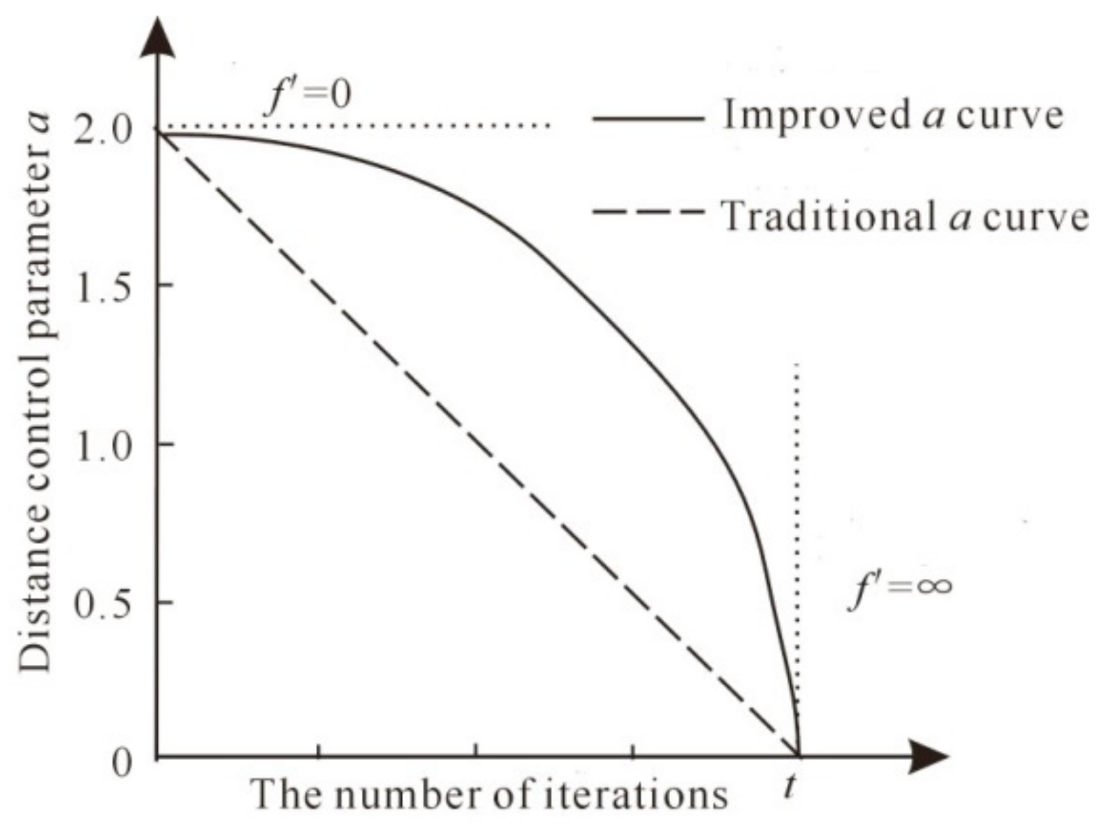
2.2.1. Improvement of Distance Control Parameters

According to the GWO, the coefficient vector $\overrightarrow{A}$ can balance local search and global search. If $\left|\stackrel{\rightharpoonup }{A}\right|\ge 1$, the search range will increase, which is conducive to global search. If $\left|\stackrel{\rightharpoonup }{A}\right|<1$, the search accuracy is strengthened, which is conducive to local search. In Equation (3), $\overrightarrow{r_1}$ is a random number in the range [0,1], hence the parameter $\overrightarrow{a}$ determines the size of $\overrightarrow{A}$ and plays a key role in the exploration and exploitation. The larger the value of $\overrightarrow{a}$, the stronger the exploration ability of the algorithm; the smaller the $\overrightarrow{a}$ value, the higher the search accuracy. In the GWO algorithm, $a=2\left(1-t/t_{max}\right)$, where t_max is the maximum number of iterations. In this study, a distance control parameter calculation method based on a circular formula is proposed; specifically, $a=2\times \sqrt{1-{\left(t/t_{max}\right)}^2}$. The variation of a with the number of iterations is shown in Figure 2.

2.2.2. Crowding Degree Added for the Archive

The archive is a simple storage unit with a maximum number and uses an archive controller to control the entry and omission of the obtained non-dominated Pareto optimal solutions from the archive. In the iteration process, if an individual in the archive dominates the new solution generated, the new solution is not be added to the archive. Conversely, if the new solution dominates one or more individuals in the archive, the new solution should replace the individual dominated. If the new solution is independent of all individuals in the archive, the new solution should be added to the archive.

In the updating process, the number of individuals in the archive will increase. However, the archive has an upper limit. Thus, to make the number of solutions in the archive not exceed the upper limit and maintain the population diversity, the MOGWO uses the grid mechanism. However, in this paper, the population in the archive is limited according to the crowding degree of the solutions in NSGA-II. The calculation process is as follows.

First, calculate the objective function $f\left(f_1,f_2,\cdots ,f_n,\right)$ of each resident in the archive, and determine the extreme values $f_i{}_{\max }$ and $f_{i\min }$ of each objective function. Then, calculate the crowding degree $D_c$ of each resident. Each solution has the attribute of crowding degree in the whole solution space:

$$D_c(j)={\displaystyle \sum _{i=1}^M\frac{f_i\left(j+1\right)-f_i\left(j-1\right)}{f_{i\max }-f_{i\min }}}$$

(12)

where $f_i\left(j+1\right)$ and $f_i\left(j-1\right)$ represent the value of the i objective function of the two adjacent individuals of j.

Finally, when the number of individuals in the archive exceeds the upper limit, the individuals with higher crowding degree, that is, the individuals with smaller $D_c$, are preferentially selected and eliminated from the archive to maintain the upper limit.

2.2.3. Improvement of the Selection Strategy for Leader Wolves

In the MOGWO, a leader selection strategy is used to select the α, β, and δ wolves. Specifically, it uses the roulette-wheel method $P_i=c/N_i$, where $P_i$ is the probability of each segment, $c$ is a constant number greater than one, and $N_i$ is the number of obtained Pareto optimal solutions in the i-th segment, to select the least crowded segments of the archive and offer one of its non-dominated solutions as α, β, and δ wolves. Moreover, it is necessary to exclude α and β from the archive temporarily when selecting the β and δ wolves to avoid selecting the same leader.

In this paper, the selection mechanism of α, β, and δ wolves is redefined. The current optimal solution is stored in the archive, and individuals are directly selected from the archive as the leader wolves. The α, β, and δ wolves are selected using the method $P_j={(D_c(j))}^C$, where C is a constant number greater than one. The smaller the $D_c$ value is, the lower is the probability of being selected.

3. Case Study

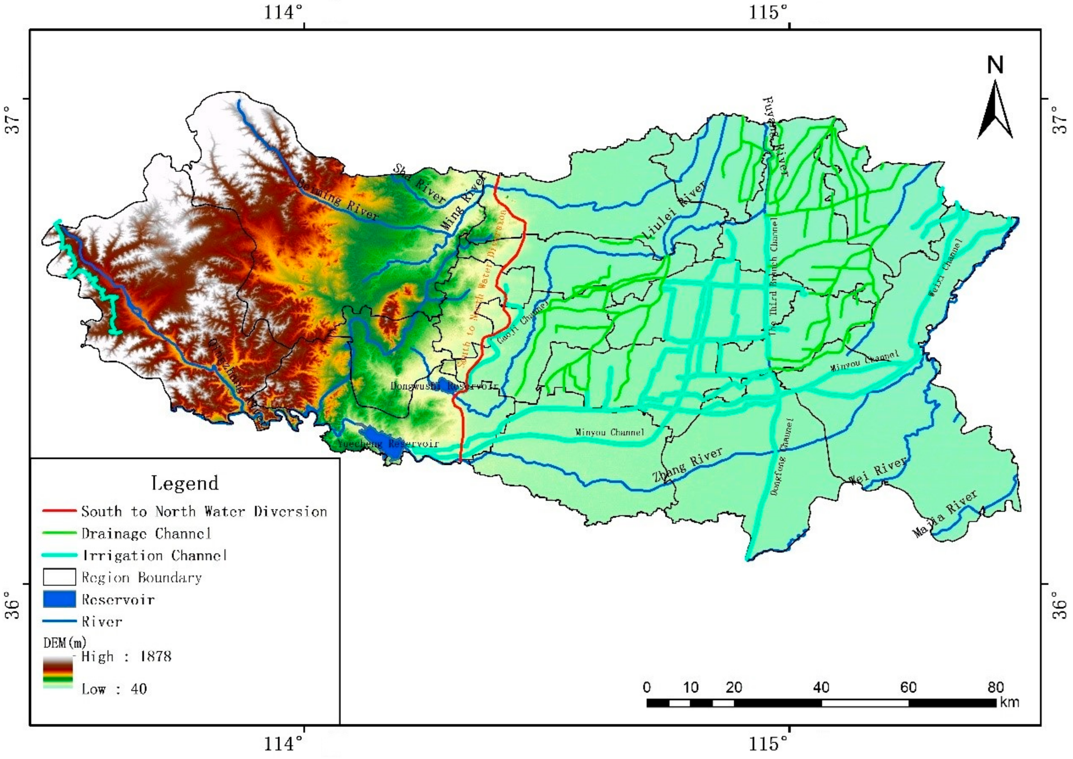
3.1. Background of the Study Area

Handan is located in the southern part of Hebei Province, China, and has a history of 3100 years, as shown in Figure 3. The population of the city is approximately 9.414 million. In addition, the area of this region is 12,047 km², in which the mountainous and plain regions cover areas of 4460 km² and 7587 km², respectively. Handan has a temperate, semi-humid, and arid continental monsoon climate. The annual average temperature is approximately 12.5–14.2 °C, and the annual average precipitation is 537.6 mm, which is concentrated from June to September. The main rivers in the territory are the Fuyang River, Zhanghe River, Weihe River, Minghe River, LiuLei River, Laozhang River, Laosha River, and Majia River. The per capita water resource in Handan is 118 m³, which is a resource-based water shortage area. Moreover, with the rapid economic development, the shortage of water resources has become the main factor that restricts and limits sustainable economic development and ensures the safety of water use.

The background conditions of water resources in Handan are weak, there are many people and limited water. Further, the temporal and spatial distribution of water resources is uneven, and it does not match the layout of productivity. With the rapid development of the social economy and the impact of global climate change, the degree of development and utilization of water resources is increasing, resulting in an imbalance between the supply and demand of water resources in the region. Simultaneously, with the decrease in water from the upstream, a large amount of groundwater is being overexploited, and the groundwater level continues to decline, forming multiple groundwater depression areas, resulting in land subsidence and frequent geological disasters. In Handan, the problem of water shortage is serious, the allocation of water resources is unreasonable, and the consumption of water in industry and agriculture is inefficient. Consequently, the adaptation and implementation of an optimal allocation technology that can scientifically and reasonably allocate the water supply in various industries and the society, realize the optimal dispatching and rational development of multiple water sources and users, and ensure the sustainable utilization of water resources and the sustainable development of the economy and society, has become a major problem to be solved because of the existing water resources and water environment conditions in this region.

3.2. Water Allocation System

Based on the characteristics of the Handan water resources system and the administrative divisions, the region is divided into 16 subregions: Shexian, Wuan, Fengfeng, Feixiang, Handan City, Yongnian, Guangping, Cheng’an, Guantao, Daming, Cixian, Weixian, Linzhang, Qiuxian, Quzhou, and Jize. Five types of water users and water sources were generalized in the optimal allocation of water resources in Handan.

The water users in Handan are divided into five categories: domestic, primary sector, secondary sector, tertiary sector, and ecological. Specifically, the primary sector covers the agriculture, forestry, livestock farming, and fisheries, the secondary sector comprises industries that produce finished and usable products and construction industries, and the tertiary sector includes catering and services.

The five water sources are local surface water, groundwater, reservoir water, externally transferred water, and recycled water. The local surface water, groundwater, and recycled water are independent water sources, whereas the reservoir water and externally transferred water are public water sources. The reservoir water includes the Yuecheng Reservoir and Dongwushi Reservoir, which supply subregions such as Feixiang, Handan City, Yongniant, Guangping, Cheng’an, Guantao, Daming, Cixian, Weixian, Linzhang, Qiuxian, Quzhou, and Jize with primary sector users, secondary sector users, and ecological users. The externally transferred water includes Yellow River-transferred water, Weihe River-transferred water, and South–North-transferred water. Thirteen subregions are supplied by the South–North-transferred water: Handan City, Feixiang, Yongnian, Guangping, Cheng’an, Guantao, Daming, Cixian, Weixian, Linzhang, Qiuxian, Quzhou, and Jize. The water users in this case include urban and rural domestic users, secondary sector users, and tertiary sector users. The Yellow River Diversion supplies subregions such as Feixiang, Guangping, Guantao, Daming, Weixian, Qiuxian, Quzhou, and Jize, and water users include primary sector users, secondary sector users, and ecological users. Three subregions are supplied by Weihe water—Guantao, Daming, and Weixian—which also have primary sector users.

3.3. Optimal Water Resource Allocation Model

The optimal water resource allocation model is established by taking the social and economic benefits as the objective functions and combining them with the corresponding constraint conditions.

3.3.1. Objective Functions

Social Benefits Target

The social benefit is usually represented indirectly by the minimum regional water shortage.

$$max{f}_1\left(x\right)=-min\left\{{\displaystyle \sum _{k=1}^K}{\displaystyle \sum _{j=1}^{J\left(k\right)}}\left[D_j^k-\left({\displaystyle \sum _{i=1}^{I\left(k\right)}}{x}_{ij}^k+{\displaystyle \sum _{c=1}^M}{x}_{cj}^k\right)\right]\right\}$$

(13)

Economic Benefit Target

The economic benefits target is characterized by the maximum net economic benefit yielded by the regional water supply.

$$\max f_2\left(x\right)=\max \left\{{\displaystyle \sum }_{k=1}^K{\displaystyle \sum }_{j=1}^{J\left(k\right)}\left[{\displaystyle \sum }_{i=1}^{I\left(k\right)}\left(b_{ij}^k-c_{ij}^k\right)x_{ij}^k{\alpha }_i^k+{\displaystyle \sum }_{c=1}^M\left(b_{cj}^k-c_{cj}^k\right)x_{cj}^k{\alpha }_c^k\right]{\lambda }_j^k\right\},$$

(14)

where $D_j^k$ is the water demand of user $j$ in subregion $k$(×106 m³); $x_{ij}^k$ and $x_{cj}^k$ are the water supplies from independent source $i$ and public source $c$ to user $j$ in subregion $k$ (×106 m³), respectively; $b_{ij}^k$ and $b_{cj}^k$ are the coefficients of efficiency per unit water supply from independent source $i$ and public source $c$ to user $j$ in subregion $k$ (CNY/m³), respectively; $c_{ij}^k$ and $c_{cj}^k$ are the coefficients of cost per unit water supply from independent source $i$ and public source $c$ to user $j$ in subregion $k$ (CNY/m³), respectively; ${\alpha }_i^k$ and ${\alpha }_c^k$ are the coefficients of water supply sequence from independent source $i$ and public source $c$ to user $j$ in subregion $k$, respectively; $K$ ($K=16$) is the total number of subregions; $I\left(k\right)$ ($I\left(k\right)=3$) is the number of the independent sources in subregion $k$; $J\left(k\right)$ ($J\left(k\right)=5$) is the number of users in subregion $k$; $M$ ($M=2$) is the total number of public sources; and ${\lambda }_j^k$ is the water supply fairness coefficient of user $j$ in subregion $k$.

3.3.2. Constraint Conditions

Water Supply Capacity Constraints

$$\begin{array}{c}\mathrm{Independent} \mathrm{water} \mathrm{resource} \\ {\displaystyle \sum _{j=1}^{J\left(k\right)}}{x}_{ij}^k\le W_i^k\end{array}$$

(15)

$$\begin{gathered} \mathrm{Public} \mathrm{water} \mathrm{resource} \\ \left\{\begin{array}{c}{\displaystyle \sum _{j=1}^{J\left(k\right)}}{x}_{cj}^k\le W_c^k\\ {\displaystyle \sum _{k=1}^K}{W}_c^k\le W_c\end{array}\right. \end{gathered}$$

(16)

Here, $W_c^k$ and $W_i^k$ are the available water supplies by public source $c$ and independent source $i$ in subregion $k$, respectively, and $W_c$ is the available water supplies by public source $c$.

Water Delivery Capacity Constraints

$$\begin{array}{c}\mathrm{Independent} \mathrm{water} \mathrm{resource} \\ x_{ij}^k\le Q_i^k\end{array}$$

(17)

$$\begin{array}{c}\mathrm{Public} \mathrm{water} \mathrm{resource} \\ W_c^k\le Q_c^k\end{array}$$

(18)

Here, $Q_i^k$ and $Q_c^k$ are the maximum water delivery capacities of the independent source $i$ and public source $c$ in the subregion $k$, respectively.

Users’ Water Demand Constraints

$$D_{jmin}^k\le {\displaystyle \sum }_{i-1}^{I\left(k\right)}{x}_{ij}^k+{\displaystyle \sum }_{c=1}^M{x}_{cj}^k\le D_{jmax}^k$$

(19)

Here, $D_{jmin}^k$ and $D_{jmax}^k$ are the minimum and maximum water demands of the user $j$ in the subregion $k$, respectively.

Non-Negative Variables

$$x_{ij}^k\ge 0$$

(20)

$$x_{cj}^k\ge 0$$

(21)

3.4. Water Demand and Supply Forecasting

Water demand forecasting is mainly used to forecast the water demand of Handan in 2035. It takes 2020 as the base year and uses the quota method [60] in combination with the long-term development planning of Handan. The water demand of the five types of water users in 2035 (p = 50%) is approximately 2740.43 × 10⁶ m³. The results are presented in

Table 1. Prediction results of water demand in Handan City in 2035 (p = 50%) (10⁶ m³).

Subregion	Domestic	Primary Sector	Secondary Sector	Tertiary Sector	Ecology	Total
Shexian	20.70	19.20	12.66	15.38	17.83	85.77
Wu’an	36.58	95.38	46.20	38.50	21.63	238.29
Fengfeng	33.30	25.76	21.86	13.25	4.23	98.40
Feixiang	20.18	120.78	8.22	9.00	5.94	164.12
Handan city	105.27	122.59	41.82	80.38	16.09	366.15
Yongnian	41.71	137.50	21.40	17.09	9.06	226.76
Guangping	14.14	66.20	6.31	7.00	3.83	97.48
Cheng’an	18.97	91.73	14.65	10.63	5.81	141.79
Guantao	15.68	87.57	3.80	9.83	5.46	122.34
Daming	37.25	177.64	6.51	14.80	12.64	248.84
Cixian	22.74	51.07	4.81	8.87	8.35	95.84
Weixian	41.96	163.57	16.50	14.88	10.19	247.10
Linzhang	29.13	145.28	10.75	12.95	8.91	207.02
Qiuxian	10.80	88.77	6.00	7.51	5.36	118.44
Quzhou	10.60	129.00	10.15	2.00	8.11	159.86
Jize	15.13	87.99	7.35	7.72	4.04	122.23
Total	474.14	1610.03	238.99	269.79	147.48	2740.43

. The water demand forecast results are used as the upper limit of the water demand for each water user type in different subregions. The lower limit is 80% of the predicted volume.

According to the water resource conditions of Handan, the available water supply in 2035 is predicted. The prediction of the available water supply of local surface water, groundwater, and recycled water directly uses the results of the Third Water Resources Evaluation in Handan [61] and the Research Report on Development and Utilization of Reclaimed Water in Handan [62]. The water supplied by the South–North Transfer Project directly uses the results from the Supporting Works Plan in Handan for the South–North Water Transfer Project (Middle Line) in Hebei Province [63]. The reservoir water, the Yellow River, and the Weihe River use the available allocated results listed in the Allocation and Utilization of Surface Water in Handan [64]. The total water supplied in Handan in 2035 is approximately 2734.13 × 10⁶ m³.

Table 2. Prediction results of available water supply in Handan in 2035 (p = 50%) (10⁶ m³).

Subregions	Local surface Water	Ground Water	Reservoir Water	Yellow River Transferred Water	Weihe Transferred Water	South–North Transferred Water	Recycled Water
Shexian	107.75	62.33					16.13
Wu’an	60.32	76.80					39.89
Fengfeng	108.53	66.56					29.00
Feixiang	2.70	19.39	√	√		10.00	14.99
Handan City	1.93	119.57	√			193.73	86.24
Yongnian	21.76	80.24	√			36.00	30.47
Guangping	0.47	15.03	√	√		7.00	10.31
Cheng’an	0.73	51.91	√			6.74	14.56
Guantao	1.36	49.55	√	√	√	7.00	10.61
Daming	1.28	107.71	√	√	√	7.90	23.81
Cixian	28.77	66.79	√			30.74	15.62
Weixian	2.03	73.12	√	√	√	21.00	28.82
Linzhang	0.30	91.46	√			7.38	19.45
Qiuxian	1.67	19.67	√	√		13.00	7.90
Quzhou	4.92	6.15	√	√		5.53	18.39
Jize	1.05	23.71	√	√		6.00	11.12
Total	345.57	929.99	560.51	138.73	30.00	352.02	377.31

lists the water supply by different water resources in each subregion of Handan in 2035 (p = 50%).

3.5. Model Parameter Determination

3.5.1. Coefficient of Water Supply Efficiency $b_{ij}^{\mathrm{k}}$

A large value is generally assigned to the water supply benefit coefficient to ensure the priority of water supply to domestic water. The efficiency coefficients for domestic water use were 800 CNY/m³. The water supply efficiency coefficients of the primary, secondary, and tertiary sectors are 15, 500, and 480 yuan/m³, respectively. The usage of ecological water can better reflect sustainable development. In addition, the value of the ecological water use efficiency coefficient is generally high, which is 800 CNY/m³.

3.5.2. Coefficient of Water Supply Cost $c_{ij}^{\mathrm{k}}$

According to the latest water supply cost, the water supply coefficients for domestic, primary, secondary, tertiary, and ecological water use are 5.2 CNY/m³, 0.2 CNY/m³, 9.0 CNY/m³, 7.0 CNY/m³, and 3.2 CNY/m³.

3.5.3. Coefficient of Water Supply Sequence ${\alpha }_i^{\mathrm{k}}$

The water supply sequence coefficient reflects the priority of the i-th water source relative to other water sources in subregion k. It can be calculated using Equation (22) [65].

$${\alpha }_{ki}=\frac{1+n_{k\max }-n_{ki}}{{{\displaystyle \sum }}_{i=1}^I\left(1+n_{k\max }-n_{ki}\right)},$$

(22)

where $n_{ki}$ is the water supply order of source $i$ in subregion $k$ and $n_{k\max }$ is the maximum order.

We calculated the water supply sequence coefficients of seven water sources in the Handan water resources allocation optimization model, in which the water supply sequence coefficients were assumed to be the same in all subregions.

Table 3. Coefficients of the water supply sequence to different water user types supplied by different water sources in Handan.

Water Supply	Domestic	Primary Sector	Secondary Sector	Tertiary Sector	Ecology
Local surface water		0.29			0.30
Ground water	0.33	0.05	0.07	0.33
Reservoir water		0.10	0.20		0.10
South to North-transferred water	0.67		0.33	0.67
Yellow River-transferred water		0.19	0.13		0.20
Weihe River-transferred water		0.14
Recycled water		0.24	0.27		0.40

lists the water supply sequence coefficients corresponding to different water user types supplied by different water sources.

3.5.4. Coefficient of Water Supply Fairness ${\lambda }_j^{\mathrm{k}}$

The water supply fairness coefficient ${\lambda }_j^k$ measures the priority of user $j$ receiving water supply relative to other users in subregion k. ${\lambda }_j^k$ and ${\alpha }_j^k$ are similar coefficients, and can be obtained using Equation (22). The priority of water supply is set as domestic, ecological, second sector, tertiary sector, and primary sector. The corresponding water supply fairness coefficients of the water users are 0.33, 0.27, 0.20, 0.13, and 0.07, respectively.

4. Results and Discussions

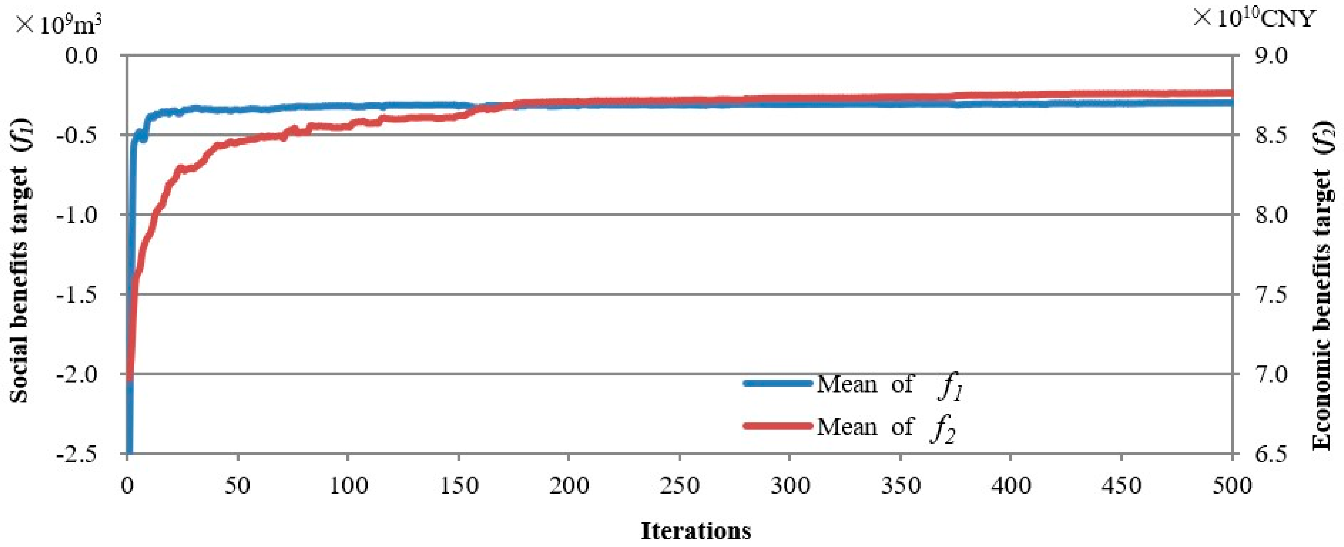
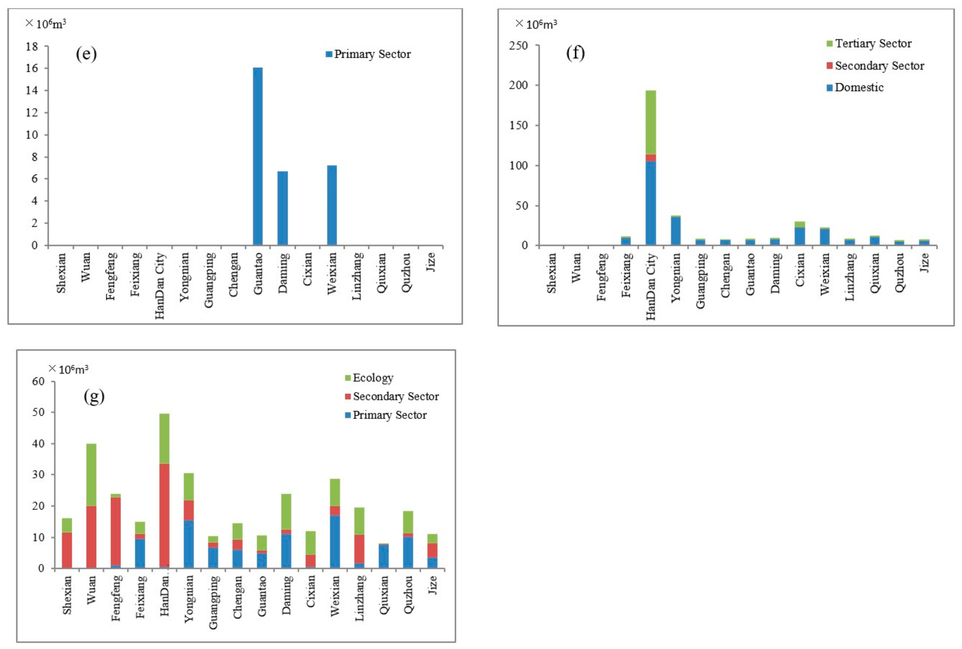
4.1. Results Analysis

In this study, AMOGWO was used to solve the multi-objective optimal allocation model of water resources in Handan. The population number was 1000, and the number of iterations was 500. MATLAB was used as a solution tool to obtain the Pareto front. Figure 4 shows the iterative process of the individual average value of the AMOGWO algorithm swarm. It is apparent that the iteration curve of the individual average value of the social benefit objective function and the economic benefit objective function tends to converge at approximately 180 iterations. After 180 iterations, it fluctuates within a small range but exhibits a stable trend. The AMOGWO algorithm has a fast convergence speed.

Moreover, we obtained the Pareto optimal solution set from the model calculation results, which provided more choices for decision-makers. Note that this solution set cannot provide the optimal option for decision-makers. The decision-makers must obtain the final scenario based on their preference and compromise between objectives. Moreover, there is a serious water shortage in Handan. Meeting the water demand of different water users is an urgent problem that needs to be solved in current water resource management. The minimum water shortage scenario should reflect the requirements of regional water resource management. Therefore, this paper chooses it as an effective scenario and analyzes it in detail.

The Handan water resources optimal allocation model in 2035 (p = 50%) yields a total water demand of 2740.43 × 10⁶ m³, a total water distribution of 2442.23 × 10⁶ m³, a water shortage of 298.20 × 10⁶ m³, and a water shortage rate of 10.9%. From the perspective of water users, the water allocated to domestic water users and ecological water users can meet the water demand and achieve a balance between supply and demand (see

Table 4. Water distribution results per user type in Handan in 2035 (p = 50%) (10⁶ m³).

Subregion	Domestic			Primary Sector			Secondary Sector			Tertiary Sector			Ecology			Total
	Demand	Allocate	Shortage	Demand	Allocate	Shortage	Demand	Allocate	Shortage	Demand	Allocate	Shortage	Demand	Allocate	Shortage	Demand	Allocate	Shortage
Shexian	20.70	20.70	0	19.20	19.20	0	12.66	12.66	0	15.38	15.38	0	17.83	17.83	0	85.77	85.77	0
Wu’an	36.58	36.58	0	95.38	58.88	−36.50	46.20	21.42	−24.78	38.50	38.50	0	21.63	21.63	0	238.29	177.01	−61.28
Fengfeng	33.30	33.30	0	25.76	25.76	0.0	21.86	21.86	0	13.25	13.25	0	4.23	4.23	0	98.40	98.40	0
Feixiang	20.18	20.18	0	120.78	92.18	−28.60	8.22	8.22	0	9.00	8.13	−0.87	5.94	5.94	0	164.12	134.65	−29.47
Handan City	105.27	105.27	0	122.59	122.59	0.0	41.82	41.82	0	80.38	80.38	0	16.09	16.09	0	366.15	366.15	0
Yongnian	41.71	41.71	0	137.50	127.42	−10.08	21.40	21.40	0	17.09	17.09	0	9.06	9.06	0	226.76	216.68	−10.08
Guangping	14.14	14.14	0	66.20	26.99	−39.21	6.31	6.31	0	7.00	7.00	0	3.83	3.83	0	97.48	58.27	−39.21
Cheng’an	18.97	18.97	0	91.73	54.10	−37.63	14.65	14.65	0	10.63	10.63	0	5.81	5.81	0	141.79	104.16	−37.63
Guantao	15.68	15.68	0	87.57	82.07	−5.50	3.80	3.80	0	9.83	9.83	0	5.46	5.46	0	122.34	116.84	−5.50
Daming	37.25	37.25	0	177.64	171.72	−5.92	6.51	6.51	0	14.80	14.80	0	12.64	12.64	0	248.84	242.92	−5.92
Cixian	22.74	22.74	0	51.07	51.07	0	4.81	4.81	0	8.87	8.87	0	8.35	8.35	0	95.84	95.84	0
Weixian	41.96	41.96	0	163.57	153.07	−10.50	16.50	16.50	0	14.88	14.88	0	10.19	10.19	0	247.10	236.60	−10.50
Linzhang	29.13	29.13	0	145.28	92.33	−52.95	10.75	10.75	0	12.95	12.95	0	8.91	8.91	0	207.02	154.07	−52.95
Qiuxian	10.80	10.80	0	88.77	83.78	−4.99	6.00	6.00	0	7.51	7.51	0	5.36	5.36	0	118.44	113.45	−4.99
Quzhou	10.60	10.60	0	129.00	116.21	−12.79	10.15	10.15	0	2.00	0.45	−1.55	8.11	8.11	0	159.86	145.52	−14.34
Jize	15.13	15.13	0	87.99	61.66	−26.33	7.35	7.35	0	7.72	7.72	0	4.04	4.04	0	122.23	95.90	−26.33
Total	474.14	474.14	0	1610.03	1339.03	−271.00	238.99	214.21	−24.78	269.79	267.37	−2.42	147.48	147.48	0	2740.43	2442.23	−298.20

). The primary, secondary, and tertiary sectors experience water shortages in some regions. The total water demand of the primary sector, total water distribution, and total water shortage are 1610.02 × 10⁶ m³, 1339.03 × 10⁶ m³, and 271.00 × 10⁶ m³, respectively, accounting for 16.8% of the water demand of the primary sector. All subregions lack water except for Shexian, Fengfeng, and Handan. Moreover, the water demand of the secondary sector is 238.99 × 10⁶ m³, and the total water allocation is 214.21 × 10⁶ m³. Note that only Wu’an fails to reach the balance of supply and demand, with a total water shortage of 24.78 × 10⁶ m³, accounting for 10.4% of the water demand of the secondary sector. The total water demand of the tertiary sector is 269.79 × 10⁶ m³, and the total water distribution is 267.37 × 10⁶ m³. Specifically, Feixiang and Quzhou do not achieve a balanced supply and demand, and the total water shortage is 2.42 × 10⁶ m³, accounting for 0.9% of the water demand of the tertiary sector. According to the statistical analysis of water shortage, there is severe water shortage in the primary sector, which accounts for 90.9% of the total water shortage, and followed by the secondary sector with a water shortage rate of 8.3%. Finally, the tertiary sector has a water shortage rate of 0.8%.

From the perspective of water supply, the total water allocation is 2442.23 × 10⁶ m³ in 2035 (p = 50%), which includes local surface water (7.0%), groundwater (35.2%), reservoir water (23.0%), Yellow River-transferred water (5.7%), Weihe-transferred water (1.2%), South–North-transferred water (14.3%), and recycled water (13.6%;

Table 5. Water distribution results per water source in Handan in 2035 (p = 50%) (10⁶ m³).

Subregion	Local Surface Water	Ground Water	Reservoir Water	Yellow River-Transferred Water	Weihe-Transferred Water	South–North-Transferred Water	Recycled Water	Total
Shexian	30.10	39.54					16.13	85.77
Wu’an	60.32	76.8					39.89	177.01
Fengfeng	25.69	48.9					23.81	98.4
Feixiang	2.70	19.39	57.85	29.72		10.00	14.99	134.65
Handan City	1.93	119.57	1.39			193.63	49.63	366.15
Yongnian	21.76	80.24	48.21			36	30.47	216.68
Guangping	0.47	15.03	21.52	3.99		6.95	10.31	58.27
Cheng’an	0.73	51.91	30.22			6.74	14.56	104.16
Guantao	1.36	49.55	9.74	22.52	16.06	7.00	10.61	116.84
Daming	1.28	107.71	85.40	10.10	6.72	7.90	23.81	242.92
Cixian	15.73	36.24	1.34			30.66	11.87	95.84
Weixian	2.03	73.12	83.89	20.52	7.22	21.00	28.82	236.6
Linzhang	0.30	91.46	35.48			7.38	19.45	154.07
Qiuxian	1.67	19.67	45.65	27.14		11.42	7.90	113.45
Quzhou	4.92	6.15	91.51	19.02		5.53	18.39	145.52
Jize	1.05	23.71	48.31	5.72		5.99	11.12	95.9
Total	172.04	858.99	560.51	138.73	30.00	350.2	331.76	2442.23

).

Figure 5a shows the allocation of different water sources to each subregion in Handan. The available water supply of local surface water is 345.57 × 10⁶ m³, and the actual water supply is 172.04 × 10⁶ m³. The supply object includes two water users—primary sector and ecological—where 147.72 × 10⁶ m³ water is supplied to primary sector and 24.32 × 10⁶ m³ for ecological environment. Meanwhile, the remaining available water supply is 173.53 × 10⁶ m³, which is concentrated in Shexian (77.65 × 10⁶ m³), Fengfeng (82.84 × 10⁶ m³), and Cixian (13.04 × 10⁶ m³).

Figure 5b illustrates the groundwater allocation in each subregion in Handan. The available water supply of groundwater resources is 929.99 × 10⁶ m³, and its actual water supply is 858.99 × 10⁶ m³, which are allocated to the domestic (222.06 × 10⁶ m³), primary (450.64 × 10⁶ m³), secondary (8.13 × 10⁶ m³), and tertiary (178.16 × 10⁶ m³).

Figure 5c shows the distribution of reservoir water, which is supplied to the users of the primary sector, secondary sector, and ecological environment. Its water supply is 560.51 × 10⁶ m³, the actual water supply is 560.51 × 10⁶ m³, and there is no surplus water. In the water distribution, 495.21 × 10⁶ m³ of water is supplied to the primary sector, 62.76 × 10⁶ m³ to the secondary sector, and 2.54 × 10⁶ m³ to the ecological environment.

The water distribution of the Yellow River mainly involves Quzhou, Weixian, Guangping, Feixiang, Daming, Guantao, Jize, and Qiuxian, which is shown in Figure 5d. The water supply of Yellow River is 138.73 × 10⁶ m³, and its actual water supply is 138.73 × 10⁶ m³. The supply targets include the users of the primary sector, secondary sector, and ecological environment. The supply of primary sector water is 119.65 × 10⁶ m³, secondary sector is 11.29 × 10⁶ m³, and ecological environment is 7.79 × 10⁶ m³. The remaining available water supply is zero.

As shown in Figure 5e, the Weihe transferred water is mostly distributed to Weixian, Daming, and Guantao for use by the primary sector. The water is completely allocated and there is no surplus; the total allocated volume is 30.0 × 10⁶ m³.

Figure 5f shows the allocation results of water transferred through the South–North Water Transfer Project to each user in each subregion in Handan. The transferred water is mostly supplied for the domestic, secondary, and tertiary sectors. The total available water supply and total allocated volumes are 352.02 × 10⁶ m³ and 350.20 × 10⁶ m³, respectively, resulting in a surplus of 1.82 × 10⁶ m³ that is not allocated for any use. The allocated volumes for domestic, secondary, and tertiary sector users are 252.08 × 10⁶ m³, 8.91 × 10⁶ m³, and 89.21 × 10⁶ m³, respectively.

The allocation results for recycled water in Handan are shown in Figure 5g. The total available water supply is 377.31 × 10⁶ m³ and the total allocated volume is 331.76 × 10⁶ m³, resulting in a surplus of 45.55 × 10⁶ m³. The reclaimed water is supplied to every subregion in Handan and is mostly allocated to the primary sector, secondary sector, and ecology in volumes of 95.81 × 10⁶ m³, 123.12 × 10⁶ m³, and 112.83 × 10⁶ m³, respectively. These account for 28.9%, 37.1%, and 34.0% of the total allocated volume, respectively.

In summary, the total water demand of all users in Handan, total available water supply, total water distribution, and water shortage are 2740.43 × 10⁶ m³, 2734.14 × 10⁶ m³, 2442.23 × 10⁶ m³, and 298.20 × 10⁶ m³, respectively. In addition, a surplus of 291.91 × 10⁶ m³ is not allocated. The reservoir water, externally transferred water (i.e., water transferred via the South–North Water Transfer Project), water imported from the Yellow River, and water from the Weihe River are fully allocated. The remaining water includes local surface water, groundwater, South–North Water transfer water, and recycled water, which are 173.53 × 10⁶ m³, 71.0 × 10⁶ m³, 1.82 × 10⁶ m³, and 45.5 × 10⁶ m³, respectively. The surplus water is concentrated in Handan City, Shexian, Fengfeng, and Cixian. The remaining water cannot be used in other regions because of the lack of a water transfer project. Among the 16 subregions of Handan, only four regions can fully meet the balance between water supply and demand: Handan City, Shexian, Fengfeng, and Cixian. However, the other 12 regions lack water in varying degrees. The highest water shortage rate is in Guangping (40.2%), followed by Cheng’an (26.5%), Wuan (25.7%), Linzhang (25.6%), Jize (21.5%), Feixiang (18.0%), Quzhou (9.0%), Guantao (4.5%), Weixian (4.2%), Qiuxian (4.2%), Yongnian (4.4%), and Daming (2.4%). Water shortages in these regions can only be alleviated by conserving water.

4.2. Comparison with NSGA-Ⅱ and MOPSO

The literature shows that the most popular multi-objective meta-heuristic algorithm is NSGA-II [18], and the second is MOPSO [66]. Consequently, the AMOGWO algorithm was compared to NSGA-II and MOPSO to evaluate its effectiveness in solving the optimal allocation model of water resources. All parameters in NSGA-II and MOPSO were set the same to ensure a fair comparison. The initialization swarm size was 1000 and the number of iterations was 500. The other parameters in MOPSO were $c_1=0.002$, $c_2=0.002$, ${\omega }^{\prime }=0.9$, and ${\omega }^{\prime \prime }=0.2$, through numerous simulation experiments.

For all three algorithms, the scenarios were chosen with preference for the minimum water shortage as the efficient solution, and to proceed with the comparative analysis. The calculation results obtained by the three algorithms are presented in

Table 6. Results for objective function values of AMOGWO, NSGA-II, and MOPSO.

Algorithm	Social Benefit (106 m3)	Economic Benefit (106 CNY)
AMOGWO	−298.20	87551.03
NSGA-II	−307.35	87272.81
MOPSO	−350.55	80116.27

. The table shows that the greatest social benefit, that is, a minimum water shortage of −298.20 × 10⁶ m³, was obtained by AMOGWO. NSGA-II ranked second, with a social benefit of −307.35 × 10⁶ m³. MOPSO has the smallest social benefit at −350.55 × 10⁶ m³. Meanwhile, the economic benefit of AMOGWO is highest, followed by NSGA-II, and the lowest is by MOPSO. The detailed allocation results are listed in

Table 7. Water distribution results of Handan obtained by NSGA-Ⅱ (10⁶ m³).

Subregions	Local Surface Water	Ground Water	Reservoir Water	Yellow River Transferred Water	Weihe Transferred Water	South To North Transferred Water	Recycled Water	Tatol
Shexian	29.54	38.12					16.11	83.77
Wu’an	56.26	76.80					39.89	172.95
Fengfeng	18.29	52.93					27.18	98.40
Feixiang	2.70	19.39	81.27	20.98		10.00	14.99	149.33
Handan City	1.93	119.40	1.62			193.39	49.81	366.15
Yongnian	21.76	80.24	15.44			36.00	30.47	183.91
Guangping	0.47	15.03	60.01	2.31		6.99	10.31	95.11
Cheng’an	0.73	51.91	54.43			6.62	14.56	128.25
Guantao	1.36	49.55	37.39	5.90	3.61	7.00	10.61	115.42
Daming	1.28	107.71	77.07	5.14	2.49	7.90	23.81	225.39
Cixian	27.87	20.66	3.05			30.74	12.59	94.91
Weixian	2.03	73.12	54.86	21.27	23.20	21.00	28.82	224.31
Linzhang	0.30	91.46	55.61			7.38	19.45	174.20
Qiuxian	1.67	19.67	36.41	27.77		13.00	7.90	106.42
Quzhou	4.92	6.15	28.16	39.98		5.53	18.39	103.13
Jize	1.05	23.71	54.28	15.38		5.89	11.12	111.43
Total	172.16	845.85	559.60	138.73	29.30	351.44	336.01	2433.08

and

Table 8. Water distribution results of Handan obtained by MOPSO (10⁶ m³).

Subregions	Local Surface Water	Ground Water	Reservoir Water	Yellow River Transferred Water	Weihe Transferred Water	South To North Transferred Water	Recycled Water	Tatol
Shexian	30.31	47.90					7.56	85.77
Wu’an	60.32	76.81					39.89	177.02
Fengfeng	24.87	62.06					11.47	98.4
Feixiang	2.70	19.39	61.14	18.30		10.00	14.99	126.52
Handan City	1.93	119.57	18.69			157.25	68.71	366.15
Yongnian	21.76	80.24	40.91			32.51	30.47	205.89
Guangping	0.47	15.03	42.56	16.79		7.00	10.31	92.16
Cheng’an	0.73	51.91	52.10			6.74	14.56	126.04
Guantao	1.36	49.31	34.91	14.87	9.07	7.00	5.82	122.34
Daming	1.28	107.71	39.57	17.74	12.34	7.90	23.81	210.35
Cixian	17.51	31.99	18.67			19.75	7.92	95.84
Weixian	2.03	73.12	47.70	18.54	8.59	21.00	28.82	199.80
Linzhang	0.30	91.46	42.97			7.38	19.45	161.56
Qiuxian	1.67	19.67	56.15	19.66		9.81	7.90	114.86
Quzhou	4.92	6.15	44.26	16.05		5.53	18.39	95.30
Jize	1.05	23.71	53.20	16.79		6.00	11.12	111.87
Total	173.21	876.03	552.83	138.74	30.00	297.87	321.19	2389.87

.

By comparing the iterative process of the three algorithms, it is apparent from Figure 4, Figure 6 and Figure 7 that although the iteration curve of AMOGWO fluctuates, the fluctuation amplitude is relatively small, and the curve converges relatively quickly. In contrast, the swarm in MOPSO does not converge at the 180th iteration, and NSGA-II becomes stable at the 340th iteration. In summary, AMOGWO has a better convergence rate and precision than NSGA-Ⅱ and MOPSO.

4.3. Discussion

As a new swarm-based meta-heuristic algorithm, the GWO algorithm has the advantages of simple principle, few parameters to adjust, easy implementation, and strong global search ability. It has been applied for the optimal allocation of water resources [67]. However, the traditional GWO has various disadvantages, including premature convergence, slow convergence speed in the later stage, and easily falling into local optimization [68]. Aiming at the shortcomings of GWO, many scholars have made improvements that improve its performance. The improvements are primarily focused on initialization population, search mechanism, and parameters. In traditional GWO, the initial population is generated based on random initialization, which cannot ensure good population diversity. Luo et al. proposed an improved GWO algorithm based on complex numerical coding [69]. Madhiarasan et al. reduced the grouping the of gray wolf population and classified the subordinate wolf group and the lowest level wolf group into one population, thereby reducing the computational complexity and increasing the convergence speed of the algorithm [70]. Long et al. used the good point set theory to initialize the population [71]. To improve the search mechanism, Saremi et al. introduced an evolutionary population dynamics (EPD) operator into GWO to enhance its exploration ability [72]. Gholizadeh et al. proposed an efficient GWO algorithm based on sequential implementation [73]. In the improvement for parameters, Long et al. balanced the exploration ability and development ability of the GWO algorithm by adjusting the adaptive value of parameter a [74]. Mittal et al. used the exponential function to attenuate a in the iterative process of the algorithm [75].

Since applying GWO algorithm directly to multi-objective optimization problems has some disadvantages, the MOGWO is proposed. It solves the problem of using GWO for multi-objective, but it does not improve the drawback of small search range and fast convergence in the early stage, and large search range and low accuracy in the later stage. To solve this problem, AMOGWO is proposed in this study. AMOGWO incorporates an improved calculation method for the distance control parameter a, adds a crowding degree for the archive, and optimizes the selection mechanism for leader wolves. It can be concluded from Figure 4 and Table 6 that after AMOGWO is applied to the multi-objective optimization of water resources allocation model in Handan, it speeds up the algorithm convergence and improves its accuracy.

In this study, we compared AMOGWO with NSGA-Ⅱ and MOPSO, which represent the most popular multi-objective meta-heuristic algorithms, to verify its superiority in the multi-objective water resources allocation model. According to previous research results, the efficiency of the water resources allocation problem can be effectively improved under NSGA-Ⅱ and MOPSO [76,77,78,79,80,81]. AMOGWO outperforms NSGA-Ⅱ and MOPSO in terms of convergence rate and solution accuracy, as evidenced in Figure 4, Figure 6 and Figure 7, and Table 6. AMOGWO thus provides a new way to solve the complex multi-objective optimization of the water resources allocation model.

5. Conclusions

In this study, an ameliorative multi-objective grey wolf optimizer (AMOGWO) was proposed, and was used on a multi-objective water resource allocation model with the maximum economic benefit and minimum water shortage as the objective function, which example is in Handan, China. The Pareto optimal frontier of the multi-objective optimization problem was obtained. In single-objective optimization, solutions can be compared easily due to the unary objective function. However, the solutions in a multi-objective space cannot be compared by the relational operators due to multi-criterion comparison metrics. Therefore, the decision-maker must obtain the final scenario based on his preference and compromise between objectives. The detailed allocation of the local surface water, groundwater, South to North transfer water, Yellow River transferred water, Weihe transferred water, and recycled water from Handan in 2035 (p = 50%) were obtained using the minimum water shortage as the criterion and selecting the best scheme from the Pareto optimal frontier. The total water demand, total water distribution, and water shortage are 2740.43 × 10⁶ m³, 2442.23 × 10⁶ m³, and 298.20 × 10⁶ m³, respectively. The total water shortage rate is 10.9%, which is concentrated in the primary sector and accounts for 90.9% of the total water shortage. The allocation results agree with the principles of water resource utilization in Handan and can provide technical support and help in decision-making for water resource allocation.

Furthermore, the AMOGWO algorithm can adapt better to the multi-objective optimal allocation of water resources and has certain advantages in convergence and iteration compared with NSGA-Ⅱ and MOPSO. This proves that the AMOGWO algorithm is effective in solving the problem of optimal allocation of water resources.

In this study, the AMOGWO algorithm only solves the optimal allocation of water resources with two objective functions. It is impossible to find a general algorithm that can solve all types of multi-objective optimization problems. Whether the AMOGWO algorithm is suitable for more than two objective functions needs to be ascertained in future work.

References

1. Vörösmary, C.J.; McIntyre, P.B.; Gessner, M.O.; Dudgeon, D.; Prusevich, A.; Green, P.; Glidden, S.; Bunn, S.E.; Sullivan, C.A.; Liermann, C.R.; et al. Global threats to human water security and river biodiversity. Nature 2010, 467, 555–561. [Google Scholar] [CrossRef]
2. Frederick, K.D.; Major, D.C. Climate change and water resources. Clim. Chang. 1997, 37, 7–23. [Google Scholar] [CrossRef]
3. Forsee, W.J.; Ahmad, S. Evaluating urban stormwater infrastructure design in response to projected climate change. J. Hydrol. Eng. 2011, 16, 865–873. [Google Scholar] [CrossRef]
4. Dawadi, S.; Ahmad, S. Evaluating the impact of demand-side management on water resources under changing climatic conditions and increasing population. J. Environ. Manag. 2013, 114, 261–275. [Google Scholar] [CrossRef] [PubMed]
5. Wang, X.; Wang, K.; Yang, W.T.; Xi, X.J.; Shi, L.Y.; Dong, W.Y.; Zhang, Q.; Zhou, Y.N. Shortage of Water Resources in China and Countermeasures. Environ. Eng. 2014, 7, 1–5. [Google Scholar]
6. Jiang, J.Q. Current situation analysis of water resources in China and Countermeasures for sustainable development. Intell. City 2019, 5, 44–45. [Google Scholar]
7. Xu, X.Y.; Wang, H.; Gan, H. Theory and Method of Macroeconomic Water Resources Planning in North China; Yellow River Water Conservancy Press: Zhengzhou, China, 1997. (In Chinese) [Google Scholar]
8. Branke, J.; KauSler, T.; Schmeck, H. Guidance in evolutionary multi-objective optimization. Adv. Eng. Softw. 2001, 32, 499–507. [Google Scholar] [CrossRef]
9. Marler, R.T.; Arora, J.S. Survey of multi-objective optimization methods for engineering. Struct. Multidiscip. Optim. 2004, 26, 369–395. [Google Scholar] [CrossRef]
10. Fang, H.S. Research of Elitist NSGA and Its Application in Regional Water Resources 0ptimal Allocation. Master’s Thesis, Zhongbei University, Taiyuan, China, 2008. (In Chinese). [Google Scholar]
11. Deb, K.; Gupta, H. Introducing Robustness in Multi-Objective Optimization; MIT Press: Cambridge, UK, 2006. [Google Scholar]
12. Wang, L.P.; Ren, Y.; Qiu, Q.C.; Qiu, F.Y. Survey on Performance Indicators for Multi-Objective Evolutionary Algorithms. Chin. J. Comput. 2021, 44, 1590–1619. [Google Scholar]
13. Coello Coello, C.A. Evolutionary multi-objective optimization: A historical view of the field. Comput. Intell. Mag. IEEE 2006, 1, 28–36. [Google Scholar] [CrossRef]
14. Coello Coello, C.A. An Updated Survey of Evolutionary Multi objective Optimization Techniques: State of the Art and Future Trends. Diabète Métabolisme 1999, 6, 109–119. [Google Scholar]
15. Whitley, D. A genetic algorithm tutorial. Stat. Comput. 1994, 4, 65–85. [Google Scholar] [CrossRef]
16. Storn, R.; Price, K. Differential evolution—A simple and efficient heuristic for global optimization over continuous spaces. J. Glob. Optim. 1997, 11, 341–359. [Google Scholar] [CrossRef]
17. Zitzler, E.; Thiele, L. Multiobjective evolutionary algorithms: A comparative case study and the strength pareto approach. IEEE Trans. Evol. Comput. 1999, 3, 257–271. [Google Scholar] [CrossRef] [Green Version]
18. Srinivas, N.; Deb, K. Muiltiobjective optimization using nondominated sorting in genetic algorithms. Evol. Comput. 1994, 2, 221–248. [Google Scholar] [CrossRef]
19. Deb, K.; Pratap, A.; Agarwal, S.; Meyarivan, T. A fast and elitist multiobjective genetic algorithm: NSGA-II. Evol. Comput. IEEE Trans. 2002, 6, 182–197. [Google Scholar] [CrossRef] [Green Version]
20. Rosenberg, R.S. Simulation of Genetic Populations with Biochemical Properties; University of Michigan: Ann Arbor, MI, USA, 1967. [Google Scholar]
21. Holland, J.H. Adaption in Natural and Artificial Systems; The University of Michigan Press: Ann Arbor, MI, USA, 1975. [Google Scholar]
22. Schaffer, J.D. Multiple Objective Optimization with Vector Evaluated Genetic Algorithms. Genetic Algorithms and Their Applications. In Proceedings of the First International Conference on Genetic Algorithms, Hillsdale, NJ, USA, 24–26 July 1985; pp. 93–100. [Google Scholar]
23. Fonseca, C.M.; Fleming, P.J. Genetic Algorithms for Multi-objective Optimization: Formulation Discussion and Generalization C. In Proceedings of the Fifth International Conference on Genetic Algorithms, San Francisco, CA, USA, 1 January 1993; pp. 416–423. [Google Scholar]
24. Zitzler, E.; Laumanns, M.; Thiele, L. SPEA2: Improving the Strength Pareto Evolutionary Algorithm C. Evolutionary Methods for Design, Optimization and Control with Applications to Industrial Problems; Springer-Verlag: Berlin, Germany, 2002; pp. 95–100. [Google Scholar]
25. Coello Coello, C.A.; Pulido, G.T. A Micro-Genetic Algorithm for Multiobjective Optimization. In Evolutionary Multi-Criterion Optimization, Proceedings of the EMO 2001, Zurich, Switzerland, 7–9 March 2001; Zitzler, E., Thiele, L., Deb, K., Coello Coello, C.A., Corne, D., Eds.; Lecture Notes in Computer Science; Springer: Heidelberg, Germany, 2001; Volume 1993. [Google Scholar] [CrossRef]
26. Rashedi, E.; Nezamabadi-Pour, H.; Saryazdi, S. GSA: A gravitational search algorithm. Inf. Sci. 2009, 179, 2232–2248. [Google Scholar] [CrossRef]
27. Webster, B.; Bernhard, P.J. A local search optimization algorithm based on natural principles of gravitation. In Proceedings of the 2003 International Conference on Information and Knowledge Engineering (IKE’03), Las Vegas, NV, USA, 23–26 June 2003; pp. 255–261. [Google Scholar]
28. Hatamlou, A. Black hole: A new heuristic optimization approach for data clustering. Inf. Sci. 2013, 222, 175–184. [Google Scholar] [CrossRef]
29. Kaveh, A.; Khayatazad, M. A new meta-heuristic method: Ray optimization. Comput. Struct. 2012, 112, 283–294. [Google Scholar] [CrossRef]
30. Shah-Hosseini, H. Principal components analysis by the galaxy-based search algorithm: A novel metaheuristic for continuous optimisation. Int. J. Comput. Sci. Eng. 2011, 6, 132–140. [Google Scholar]
31. Moghaddam, F.F.; Moghaddam, R.F.; Cheriet, M. Curved space optimization: A random search based on general relativity theory. arXiv 2012, arXiv:1208.2214. [Google Scholar]
32. Kennedy, J.; Eberhart, R. Particle swarm optimization. In Proceedings of the 1995 IEEE International Conference on Neural Networks, Perth, WA, Australia, 27 November–1 December 1995; 4, pp. 1942–1948. [Google Scholar]
33. Dorigo, M.; Birattari, M.; Stutzle, T. Ant colony optimization. IEEE Comput. Intell. 2006, 1, 28–39. [Google Scholar] [CrossRef]
34. Li, X.L.; Shao, Z.J.; Qian, J.X. An optimizing method based on autonomous animats: Fish-swarm algorithm. Syst. Eng. Theory Pract. 2002, 22, 32–38. (In Chinese) [Google Scholar]
35. Pan, W.T. A new fruit fly optimization algorithm: Taking the financial distress model as an example. Knowl. Based Syst. 2012, 26, 69–74. [Google Scholar] [CrossRef]
36. Mirjalili, S.; Lewis, A. The whale optimization algorithm. Adv. Eng. Softw. 2016, 95, 51–67. [Google Scholar] [CrossRef]
37. Zhu, H.P.; Li, W.J. Multiobjective Structural Optimization with Pareto Genetic Algorithm. J. Northwestern Polytech. Univ. 2001, 19, 152–155. [Google Scholar]
38. Kipouros, T.; Jaeggi, D.M.; Dawes, W.N.; Parks, G.T.; Savill, A.M.; Clarkson, P.J. Biobjective design optimization for axial compressors using Tabu Search. AIAA J. 2008, 46, 701–711. [Google Scholar] [CrossRef]
39. Luh, G.C.; Chueh, C.H. Multi-objective optimal design of truss structure with immune algorithm. Comput. Struct. 2004, 82, 829–844. [Google Scholar] [CrossRef]
40. Guo, H.F.; Ma, H.B.; Dong, Z.C.; Qin, X.B. The Aplication of Improved Multi-objective Particle Swarm Optimization Algorithm to Water Resources Allocation of Poyang Lake. China Rural Water Hydropower 2012, 10, 61–64. (In Chinese) [Google Scholar]
41. Wu, A.H. Research and Application of Multi-Objective Ant-Genetic Algorithm for Region Water Resources Optimal Allocation. Comput. Knowl. Technol. 2007, 23, 1392–1393+1398. (In Chinese) [Google Scholar]
42. Liu, B.; Sha, J.X. Application of Improved Artificial Fish Swarm Algorithm in Optimal Allocation of Water Resources. Yellow River 2017, 39, 58–62. (In Chinese) [Google Scholar]
43. Yan, Z.H.; Sha, J.X.; Liu, B.; Tian, W.; Lu, J.P. An Ameliorative Whale Optimization Algorithm for Multi-Objective Optimal Allocation of Water Resources in Handan, China. Water 2018, 10, 87. [Google Scholar] [CrossRef] [Green Version]
44. Wolpert, D.H.; Macready, W.G. No free lunch theorems for optimization. IEEE Trans. Evol. Comput. 1997, 1, 67–82. [Google Scholar] [CrossRef] [Green Version]
45. Mirjalili, S.; Mirjalili, S.M.; Lewis, A. Grey wolf optimizer. Adv. Eng. Softw. 2014, 69, 46–61. [Google Scholar] [CrossRef] [Green Version]
46. Kalita, K.; Shinde, D.; Chakraborty, S. Grey wolf optimizer-based design of ventilated brake disc. J. Braz. Soc. Mech. Sci. Eng. 2021, 43, 405. [Google Scholar] [CrossRef]
47. Zakian, P.; Ordoubadi, B.; Alavi, E. Optimal design of steel pipe rack structures using PSO, GWO, and IGWO algorithms. Adv. Struct. Eng. 2021, 24, 2529–2541. [Google Scholar] [CrossRef]
48. Diastivena, D.; Wahyuningsih, S.; Satyananda, D. Grey Wolf Optimizer algorithm for solving the multi depot vehicle routing problem and its implementation. J. Phys. Conf. Ser. 2021, 1872, 012001. [Google Scholar] [CrossRef]
49. Zhang, S.; Zhou, Y.; Li, Z.; Pan, W. Grey wolf optimizer for unmanned combat aerial vehicle path planning. Adv. Eng. Softw. 2016, 99, 121–136. [Google Scholar] [CrossRef] [Green Version]
50. Zhang, Z.; Hong, W. Application of variational mode decomposition and chaotic grey wolf optimizer with support vector regression for forecasting electric loads. Knowl. Based Syst. 2021, 228, 107297. [Google Scholar] [CrossRef]
51. Ghalambaz, M.; Jalilzadeh, Y.R.; Davami, A.H. Building energy optimization using grey wolf optimizer (GWO). Case Stud. Therm. Eng. 2021, 27, 101250. [Google Scholar] [CrossRef]
52. Emary, E.; Zawbaa, H.M.; Grosan, C.; Hassenian, A.E. Feature Subset Selection Approach by Gray-Wolf Optimization. In Afro-European Conference for Industrial Advancement. Advances in Intelligent Systems and Computing; Abraham, A., Krömer, P., Snasel, V., Eds.; Springer: Cham, Switzerland, 2015; p. 334. [Google Scholar]
53. Kumar, A.; Lekhraj; Singh, S.; Kumar, A. Grey wolf optimizer and other metaheuristic optimization techniques with image processing as their applications: A review. IOP Conf. Ser. Mater. Sci. Eng. 2021, 1136, 012053. [Google Scholar] [CrossRef]
54. Wang, X.; Li, Z.S.; Kang, H.; Huang, Y.P.; Gai, D. Medical Image Segmentation using PCNN based on Multi-feature Grey Wolf Optimizer Bionic Algorithm. J. Bionic Eng. 2021, 18, 711–720. [Google Scholar] [CrossRef]
55. Sathiyabhama, B.; Kumar, S.U.; Jayanthi, J.; Sathiya, T.; Ilavarasi, A.K.; Yuvarajan, V.; Gopikrishna, K. A novel feature selection framework based on grey wolf optimizer for mammogram image analysis. Neural Comput. Appl. 2021, 33, 14583–14602. [Google Scholar] [CrossRef]
56. Niu, W.; Feng, Z.; Liu, S.; Chen, Y.; Xu, Y.; Zhang, J. Multiple Hydropower Reservoirs Operation by Hyperbolic Grey Wolf Optimizer Based on Elitism Selection and Adaptive Mutation. Water Resour. Manag. 2021, 35, 573–591. [Google Scholar] [CrossRef]
57. Dahmani, S.; Yebdri, D. Hybrid Algorithm of Particle Swarm Optimization and Grey Wolf Optimizer for Reservoir Operation Management. Water Resour. Manag. 2020, 34, 4545–4560. [Google Scholar] [CrossRef]
58. Mirjalili, S.; Saremi, S.; Mirjalili, S.M.; Coelho, L. Multi-objective grey wolf optimizer: A novel algorithm for multi-criterion optimization. Expert Syst. Appl. 2015, 47, 106–119. [Google Scholar] [CrossRef]
59. Cui, M.L.; Du, H.W.; Wei, Z.L.; Li, C. Research on improved strategy for multi-objective grey wolf optimizer. Comput. Eng. Appl. 2018, 54, 156–164. (In Chinese) [Google Scholar]
60. Hebei Provincial Water Resources Department; Hebei Provincial Administration of Quality and Technical Supervision. Hebei Province Water Use Quota; Hebei Provincial Water Resources Department: Shijiazhuang, China, 2016. (In Chinese)
61. Hebei Handan Hydrology and Water Resources Survey Bureau. Assessment of Water Resources in Handan (Third); Hebei Handan Hydrology and Water Resources Survey Bureau: Handan, China, 2019; pp. 71–165. (In Chinese) [Google Scholar]
62. Hebei University of Engneering. Research Report on Development and Utilization of Reclaimed Water in Handan; Hebei University of Engneering: Handan, China, 2018; pp. 213–219. (In Chinese) [Google Scholar]
63. Handan Water Resources and Hydropower Survey and Design Institute. The Planning of Handan in the South to North Water Transfer Project (Middle Line) of Hebei Province; Handan Water Resources and Hydropower Survey and Design Institute: Handan, China, 2002; pp. 102–110. (In Chinese) [Google Scholar]
64. Water Conservancy Bureau of Handan. Allocation and Utilization of Surface Water in Handan; Water Conservancy Bureau of Handan: Handan, China, 2020; pp. 21–22. (In Chinese) [Google Scholar]
65. Zeng, F.C. Research on Supply-requirement Analysis and Optimized Allocation of Water Resources in Xi’an City. Master’s Thesis, Chang’an University, Xi’an, China, May 2008. (In Chinese). [Google Scholar]
66. Coello, C.A.C.; Pulido, G.T.; Lechuga, M.S. Handling multiple objectives with particle swarm optimization. Evol. Comput. IEEE Trans. 2004, 8, 256–279. [Google Scholar] [CrossRef]
67. Chen, J.H.; Cheng, G. Application of GWO-projection suit model to water allocation for Yunnan Province. J. China Three Gorges Univ. (Nat. Sci.) 2016, 38, 29–35. [Google Scholar]
68. Long, W.; Cai, S.H.; Jiao, J.J.; Wu, T.B. An Improved GWO. Acta Electron. Sin. 2019, 47, 171–177. [Google Scholar]
69. Qifang, L.; Sen, Z.; Zhiming, L.; Yongquan, Z. A novel complex-valued encoding grey wolf optimization algorithm. Algorithms 2015, 9, 4. [Google Scholar]
70. Madhiarsan, M.; Deepa, S.N. Long-Term Wind Speed Forecasting using Spiking Neural Network Optimized by Improved Modified Grey Wolf Optimization Algorithm. Int. J. Adv. Res. 2016, 4, 356–368. [Google Scholar] [CrossRef] [Green Version]
71. Long, W.; Zhao, D.Q.; XU, S.J. Improved grey wolf optimization algorithm for constrained optimization problem. J. Comput. Appl. 2015, 35, 2590–2595. (In Chinese) [Google Scholar]
72. Saremi, S.; Mirjalili, S.Z.; Mirjalili, S.M. Evolutionary population dynamics and grey wolf optimizer. Neural Comput. Appl. 2015, 26, 1257–1263. [Google Scholar] [CrossRef]
73. Gholizadeh, S. Optimal design of double layer grids considering nonlinear behaviour by sequential grey wolf algorithm. J. Optim. Civ. Eng. 2015, 5, 511–523. [Google Scholar]
74. Long, W.; Liang, X.; Cai, S. A modified augmented Lagrangian with improved grey wolf optimization to constrained optimization problems. Neural Comput. Appl. 2016, 28, 421–438. [Google Scholar] [CrossRef]
75. Mittal, N.; Singh, U.; Sohi, B.S. Modified Grey Wolf Optimizer for Global Engineering Optimization. Appl. Comput. Intell. Soft. Comput. 2016, 2016, 7950348. [Google Scholar] [CrossRef] [Green Version]
76. Sha, J.X. Application of Improved NSGA-Ⅱ in Optimal Allocation of Water Resources in Xingtai City. Water Resour. Power 2018, 36, 21–26. (In Chinese) [Google Scholar]
77. Sha, J.X.; Liu, B.; Xie, X.M.; Lu, H.Y. Study of water resources optimal allocation based on particle swarm optimization. Water Resour. Power 2012, 30, 35–37+69. (In Chinese) [Google Scholar]
78. Yan, Z.H.; Liu, B.; Zhang, T.; Sha, J.X.; Nie, H.-J. Study of water resources optimal allocation based on multi-objective particle swarm optimization. Water Resour. Power 2014, 32, 35–37+45. (In Chinese) [Google Scholar]
79. Qu, G.D.; Lou, Z.H. Application of particle swarm algorithm in the optimal allocation of regional water resources based on immune evolutionary algorithm. J. Shanghai Jiaotong Univ. Sci. 2013, 18, 634–640. [Google Scholar] [CrossRef]
80. Zhang, L.; Xu, Z.X.; Zhang, Z.G. Rational allocation of water resources based on particle swarm optimization. J. China Hydrol. 2009, 29, 41–45+23. (In Chinese) [Google Scholar]
81. Chen, X.N.; Duan, Q.C.; Qiu, L.; Huang, Q. Application of large scale system model based on particle swarm optimization to optimal allocation of water resources in irrigation areas. Transact. CSAE 2008, 24, 103–106. (In Chinese) [Google Scholar]
Figure 1. Social hierarchy of gray wolves.
Water 14 00063 g001
Figure 2. Variation of distance control parameter a   with the number of iterations.
Water 14 00063 g002
Figure 3. Map of the administrative division and water supply system in Handan.
Water 14 00063 g003
Figure 4. Iterative process of the individual average value of AMOGWO swarm.
Water 14 00063 g004
Figure 5. Distribution results of different water users supplied by each water source. (a) Local surface water, (b) groundwater, (c) reservoir water, (d) Yellow River-transferred water, (e) Weihe-transferred water, (f) South–North-transferred water, and (g) recycled water.
Water 14 00063 g005aWater 14 00063 g005b
Figure 6. Iterative process of NSGA-II.
Water 14 00063 g006
Figure 7. Iterative process of MOPSO.
Water 14 00063 g007