
On the Understanding of the Hydrodynamics and the Causes of Saltwater Intrusion on Lagoon Tidal Springs
by
 , , and
Roger Pacheco-Castro
1,2,3 ,
,
Paulo Salles
2,3,*,
Cesar Canul-Macario
2 and
Alejandro Paladio-Hernandez
2 1
Catedras-CONACyT, Consejo Nacional de Ciencia y Tecnología, Ciudad de México 03940, Mexico
2
Laboratorio de Ingeniería y Procesos Costeros, Instituto de Ingeniería, Universidad Nacional Autónoma de México, Puerto de Abrigo S/N, Sisal 97355, Mexico
3
Laboratorio Nacional de Resiliencia Costera, Sisal 97355, Mexico
*
Author to whom correspondence should be addressed.
Water 2021, 13(23), 3431; https://doi.org/10.3390/w13233431
Submission received: 5 October 2021
/
Revised: 16 November 2021
/
Accepted: 23 November 2021
/
Published: 3 December 2021
(This article belongs to the Special Issue Coastal Aquifers: Seawater/Saltwater Intrusion)
Abstract
:Springs are common features on the Yucatán coast. They can discharge either under the sea (submarine) or inland in coastal lagoons and wetlands. Previous observations of a coastal lagoon located on the northern Yucatán Peninsula (La Carbonera) reported sea water intrusion on a spring that discharge on a coastal lagoon (lagoon tidal spring). The saltwater intrusion occurs when the tide is at its lower level, which is the opposite to what has been reported for submarine springs in the Yucatán Peninsula. In this study, the hydrodynamics of the spring is analyzed and the driving forces controlling the seawater intrusion are identified and discussed. Time series of water levels, salinity, and velocity measurements in the lagoon, the aquifer, and the spring are analyzed by means of tide component decomposition and cross-correlations analysis of the tide signals. Results show that the main driving forces causing the intrusion are the density differences and pressure head gradients, and the mechanisms influencing the driving forces driving those differences are the tides, the friction in the lagoon, and the confinement of the aquifer; other mechanisms are discussed to present a complete idea of the complexity of the interactions between the coastal aquifer, the coastal lagoons, and the sea.
1. Introduction
In the state of Yucatán, México, submerged springs are common features that are located either on the sea (submarine) or inland on coastal lagoons and wetlands. On submarine springs, one important factor that controls the discharge is the tide, and during spring high tides, the flow may reverse, causing salt water to intrude the spring. Recent studies in coastal lagoons have reported an opposite behavior in lagoon springs [1,2] in which the flow reversal occurs during spring low tide, which is a behavior that is apparently counterintuitive; see below. This paper studies the lagoon spring hydrodynamics, compares it to submarine springs, and analyzes the factors that cause saltwater intrusion through the spring.
Springs are points of groundwater discharge on the land or surface water bodies, and they are important features of aquifer systems, particularly in karst aquifers [1,2,3]. COSOD [4] estimated that half of the total infiltration discharge into the oceans occurs in the form of submarine springs. Springs on karst aquifers are some of the largest in the world; for example, the Dumanli Spring in Turkey has a mean discharge of 50 m3/s [5], and Scott et al. [6] report 33 springs in Florida with an average discharge flow larger than 2.8 m3/s. Springs have been used as a water resource for thousands of years as archeological evidence shows [3,7,8], they may be an important component in water budgets, and they have a significant influence on the environments where they discharge [4,9,10,11]. In the case of karst springs, it has been proved that they can also provide information about the aquifer structure [1,2].
There are many classifications of springs proposed in the literature, depending on the discharge rate, discharge uniformity, hydraulic characteristics, geology, water quality, and water temperature [3,12], and Bogli [13] presented a classification only for karst springs. Recent studies propose a more interdisciplinary classification considering the ecosystems that depends on the groundwater discharge [9]. When the springs discharge into other water bodies, they are commonly called submerged [13]. It is interesting to note that in terms of submerged springs, Bogli [13] only considers submarine (discharge in the sea) springs and sublacustrine (discharge in lakes) springs; however, it does not consider springs that discharge in other surface water bodies. For instance, in the Yucatán coast, there are springs that discharge in lagoons [14,15], and the Spring Creek springs discharge into an estuary [16,17]. In terms of the hydraulic characteristics, springs are classified as gravity springs if they occur at the intersection of the water table with the surface and artesian springs when the discharge occurs from confined conditions [3,12]. The latter are of particular interest for this study given that, as we will discuss in the next section, the springs of the Yucatán peninsula occur on a narrow confining layer on the coast [14,18]. In terms of the outflow, the categories proposed by Bogli [13] are perennial, periodic, rhythmic, and episodic springs. The discharge of periodic springs depends on the periodicity of the recharge [13]. Rhythmic springs, also called ebb and flow (or flood) springs or intermittent springs, are characterized by having a strong variation in the outflow [12,13,19]. This type of springs is not common, and in the US, only 23 were identified by [12]. Bogli [13] describes this phenomenon as dependent on the physical setting called the syphon effect [13,19]. Ref. [19] further analyzes different types of rhythmic springs based on the aquifer recharge periodicity. Episodic springs discharge only when there is an extreme water level on the aquifer [13]. Estavelle is another name used for describing karst openings with dual functions: at low head in the aquifer, they are sinks, and when the head in the aquifer is high, they become springs [3,12,13]. The springs considered in this work show a periodic behavior in the discharge [15,20]; however, the periodicity is due to the tides and not caused by the precipitation periodicity nor the siphon effect, and they can behave as estavelles, as discussed later. There is no consensus on the terminology to refer to this type of springs: Williams [21] call the Waikoroupupu springs “tidal” springs because they show tidal variability. The work of McCormac [22] defines intertidal springs as “springs alternating from free draining to wholly submerged springs. As such, it is important to designate the discharge from these springs as ‘intertidal’”. Schuler et al. [23] refers to the discharge that occurs on the shore and influenced by the tides as “submarine intertidal discharge”. The spring discussed in this study (a) behaves as an estavelle, in the sense that becomes a sink under some conditions (shown later), (b) is a submerged spring since it never drains freely because of the presence of the lagoon, (c) is artesian, and (d) shows a tidal periodicity (not a rhythmic spring in the sense discussed before). Given the above, the spring in this study will be referred to as lagoon tidal spring.
Holliday et al. [24] analyze the geologic controls on submarine groundwater discharge from a confined aquifer and Fleury et al. [25] present a review of submarine springs located in karstic aquifers. They found that the main mechanisms involved in the hydrodynamics of the submarine springs are the aquifer discharge and the saline intrusion through conduits. In the case of the Yucatán peninsula, Mexico, Valle-Levinson et al. [20] studied the discharge at the Xbuya-Ha submarine spring (in the coastal ocean, roughly 350 m from the coastline) in the northern coast of Yucatán State. They found that the discharge was inversely related to the tide: low tide produced the strongest discharge, and at high tide, the discharge weakened and could even reverse. Similar results were reported for a submarine spring in Australia [24]. Parra et al. [26,27] also report similar results for springs in the Mexican Caribbean coast. The factors controlling the spring dynamics identified on those studies were the piezometric gradient, the water level, and the density differences [20,24]. The Spring Creek springs discharge into an estuary, and all the springs experiment flow reversal on high tides [7,16,17]. Similar results are reported for the Kinvara West intertidal springs in Ireland [22]. Both cases are analogous to the submarine springs reported by other authors [20,24,26]. However, this behavior is the opposite of what is observed in the springs located at La Carbonera coastal lagoon in Yucatán: the flow may reverse at the spring low tides [28,29,30]. Febles and Batllori [28] performed measurements of salinity, water levels, and flow rates during May and June of 1993 and reported the variations of water levels in the spring with the purpose of analyzing the advantages and disadvantages of having a channel in the Peten (a roughly circular patch of brackish water vegetation surrounding springs in coastal lagoons and wetlands in the Yucatán coast) and cleaning the spring debris to increase the flow rate. They observed that saltier water was getting into the spring during what they called extreme low tide. Rey [30] also found this phenomenon when collecting data for modeling of the hydrodynamics in La Carbonera lagoon.
Febles and Batllori [28] and Rey [30] propose that the hydrodynamic behavior of the spring discharge was caused by the sea tide variation, the recharge/discharge of the aquifer and aquifer confinement. Given the ecological relevance of the coastal lagoons for Yucatán, the potential threat caused by the brackish/hypersaline saltwater intrusion and the desire to understand the difference in behavior of those inland coastal springs, as opposed to the offshore springs, a more complete sampling campaign was carried out to investigate the hydrodynamics of the spring and the causes of the saltwater intrusion. The objectives of this work are as follows: (a) to study the hydrodynamics of a lagoon tidal spring, (b) determine the driving forces influencing the saltwater intrusion, and to (c) identify the mechanisms influencing the driving forces of saltwater intrusion. Concurrent field observations across the aquifer, lagoon, Peten, and the sea are employed to understand the complex interactions in this coastal spring.
2. Materials and Methods
2.1. Study Area
The study area is located in the northwest of the Yucatán State, Mexico (Figure 1). The aquifer of the Yucatán Peninsula is developed in a carbonate platform, being composed of limestone, marl, and gypsum of high heterogeneity [31,32,33]. The surficial geology (Figure 1b) shows the presence of tertiary and quaternary deposits. Quaternary deposits are not consolidated and are composed mainly of limestones with mollusks, sandbacks, clays, and soils. Tertiary deposits are composed mainly of limestone deposits from the Carrillo Puerto formation [34,35]. The aquifer consists of a lens of fresh water under-laid by saline water [18,32,33], the depth of the saline interface on well P5 is about 15 m and increases landwards [36]. The regional flow is from the southeast to the northeast, toward the coast, and shows a low hydraulic gradient (of the order of 10−2 m/km [14]). According to [33], the rain season in Yucatán State is from May to November, the amount of rain for the state varies from 444 to 1227 mm, and the precipitation increases from north to south and from west to east (the study zone is in a zone with the lowest precipitation rates). The mean average temperature is 24.5 to 25.5 °C and the average annual evapotranspiration is 500 to 1100 mm, and follows the same pattern as the precipitation [14,33]. Mixed tides influence the study area with a dominance of diurnal tides ranging between 0.15 and 0.75 during neap and spring tides, respectively [27].
In this area, the springs occur as the result of fractures in a narrow confining layer, which consist of a cemented material locally known as “caliche”. The exact extent inland and offshore of the caliche layer is unknown; it has been proposed that it extends 5 to 7 km inland and 3 km offshore [18], and previous research suggests that the width decreases toward the east [37]. The thickness of the confining layer is estimated to be between 0.5 and 1.4 m [31,32,33,38]. Villasuso [37] shows the existence of a low permeability layer of sand limestones inland, which can act as a semi-confining layer that extends further inland. Similar results are reported by Canul-Macario et al. [36], where this layer extends more than 12 km from the coast at Sisal.
Given its karstic nature, the aquifer is highly vulnerable to surficial contamination [33,39,40]. Old domestic and municipal sewage (with no proper sceptic tanks or water treatment), untreated residues from animals, and fertilizers are the major sources of groundwater pollutants [31,32,41,42]. In addition, the coastal zone of Yucatán State has experienced an increase in demography and tourism and is also subject to sea-level rise (2.5 ± 1.2 mm/year on average according to [43]), which increases the risk of causing severe damage to this resource [44,45,46,47].
The coastal springs discharge freshwater in lagoons (or wetlands) or in the sea. Coastal lagoons of Yucatán are important because they are the habitats of several species of animals and vegetation [48,49] and are increasingly used for low-impact tourism. Those systems suffer from high environmental variability over short time scales because they are a transition zone between the karst lands and the sea, making hydrodynamics complex [49,50]. Significant changes in the lagoon hydrodynamics may result in soil erosion and loss of endemic species [14]. The northern Yucatán State coast has a total of 12 single-inlet shallow coastal lagoons with large areas of mangroves and wetlands [49]. In particular, La Carbonera (Figure 1b,c) is a coastal lagoon located in the northwest part of the Yucatán State (Figure 1a); it is composed of a shallow water body with an average depth of 0.5 m, an extension of 16 km2, and watersheds that separate it from adjacent intermittent water bodies (marshes and wetlands). The lagoon is connected to the sea with a single inlet and communicates with the adjacent wetlands during spring high tides occurring during the rainy season. The La Carbonera lagoon can be considered a chocked lagoon as proposed by Kjerfve [51], which is characterized for having a single long narrow channel that acts as a filter to tidal currents and water levels. The lagoon is important from an ecological point of view, being the habitat of different species of fish, birds, and vegetation, such as rose flamingoes and mangroves [14,29,30,50,52]. In addition, there is a significant interaction with the confined aquifer through varying-size springs that discharge freshwater into the lagoon, which is often surrounded by ecosystems locally known as Petenes, which are roughly circular patches of freshwater vegetation (Figure 1c) surrounded by saline or hypersaline water that provide thermohaline gradients in the lagoons [14,30].
The spring subject of this study is located inside the biggest Peten in La Carbonera lagoon (shown as a big patch of vegetation; Figure 1b), and its discharge forms a pool of roughly 60 m2 and an average depth of 2 m (between C3 and SP in Figure 1d), which in turn discharges to the lagoon through a winding narrow channel (on average 1 m deep, 2.5 m wide, and approximately 550 m long) between the spring (SP) and the lagoon at C1 (Figure 1d). This is the spring where the saltwater intrusion was first reported [28,30]. The spring opens at the bottom of the pool, right at SP in Figure 1d. This is the place where a conductivity sensor was placed. The opening looks like a small cave with a small opening (zone where confinement fractures), but no diver could go deep, because there are many rocks and debris where the water seeps through. The spring channel slope is irregular but on average tilted toward the lagoon, with a lower elevation at C1 with respect to C3 (Figure S1 in Electronic Supplementary Materials (ESM)).
Figure 1.
(a) Yucatán Peninsula and its geology. The study site is highlighted in the red square, monitoring stations are shown as red dots, and meteorological stations are shown as blue triangles. (b) Zoom to the red square in panel (a): overview of the study zone and its geology. (c) Zoom to the green square in panel (b): La Carbonera coastal lagoon. The Peten and the spring location are indicated by the white arrow (SP). (d) Zoom to the yellow square in panel (b), next to the white arrow showing the spring and Peten location: the white line corresponds to the channel that connects the spring SP to the lagoon and the contour of the spring pool (between SP and C3). Imagery from Google Earth and the Mexican Geological Service (SGM) [53].

2.2. Data Acquisition and Analysis
With the aim of studying the hydrodynamics of the spring and the main factors responsible for the salt intrusion during spring low tide, a sampling campaign was carried out between November 2017 and January 2018. We can classify the monitored locations in three sets. The first set corresponds to locations in the Peten channel and spring: C1 (channel entrance), C2 (mid channel), C3 (channel end), and SP (spring); the second set corresponds to locations in the lagoon L1 and L2 (Figure 1c,d), and the third set corresponds to wells in adjacent areas of the aquifer (B9 and P5, Figure 1b). The undisturbed tide was monitored at SE (Figure 1c).
The measured parameters for the lagoon and Peten channel were pressure, electrical conductivity, and temperature, using HoBo® pressure and conductivity sensors (Onset, Cape Cod, MA, USA), with one recorded measurement every 10 min (only P5 has measurements each 30 min). The electrical conductivity was converted to salinity in practical salinity units psu [54] using the HoBoware Pro software (version 3.7.4, Onset, Cape Cod, MA, USA) and corrected for sensor drift using electrical conductivity measurements from a LS600YSI® sonde (YSI Inc./Xylem Inc., Yellow Springs, OH, USA). For the monitoring locations at the lagoon and Peten channel, pressure was converted to water height, corrected for atmospheric pressure, and a calculated density (estimated with the conductivity measurements), using TEOS 10 routines for Python (Python Software Foundation, Wilmington, NC, USA) [55]. The sensors were placed close to the bottom and referenced to the same vertical datum. In the case of the wells, pressure measurements were converted to hydraulic head and referenced to the same vertical datum.
At station C3 near the spring, a Nortek Vector acoustic current meter (Nortek, Rud, Norway) was deployed (close to the bottom), measuring the x, y, and z components of the flow velocity. The freshwater discharge at SP was so clear (absence of suspended matter) that the measured velocities with the acoustic instrument were noisy. Following the instrument guidelines, the data with a low number of counts were removed, after which the velocities were rotated to align the x-axis with the axis of maximum variation (i.e., in the direction of the spring flow). One measurement was taken each 10 min with 20 bursts per sample.
Other datasets are available that provide some insight of the hydrodynamics of the spring and evidence of the salt intrusion. The first one is a sampling campaign between May and June 2016 (dry season, i.e., low freshwater input from the aquifer), in which only three sites were monitored: one on the sea (SE), one at the entrance of the channel (C1), and one at the end of the channel (C3), for which the pressure sensors were not vertically referenced. The second dataset corresponds to another sampling campaign between September and October 2016 (end of rainy season, i.e., large freshwater discharge from the aquifer), in the same locations as in the previous dataset. Only salinity measurements are considered in this study.
Finally, precipitation records were obtained from meteorological stations of the University Network of Atmospheric Observatories from the National Autonomous University of Mexico (https://www.ruoa.unam.mx/, accessed on 4 July 2021) [56]. The stations are located in the State capital Merida and two other small coastal towns close to the study site: Progreso and Celestun (Figure 1a).
2.3. Tide Component Extraction
Tides are an important mechanism to be considered in studies of confined coastal aquifers and lagoons with connection to the sea. Tides play a key role in the hydrodynamics of those systems [57,58,59]. The tidal signal can be decomposed in two parts: the first caused by the gravitational forces of the moon, earth, and sun, which is known as astronomic tide, and the second caused by meteorological factors (atmospheric pressure and wind stress over the coastal ocean) that affect the sea level, which is called meteorological tide. Given that the movement of the earth, sun, and moon is well understood, the astronomic tide can be predicted accurately. For a given site, the astronomic tide is a sum of periodic components,
where is the sea tide water level (m), is the mean sea water level (m), is the frequency of each astronomic component (1/h), and are the amplitude and phase, respectively. Harmonic analysis is performed on a set of water level observations to estimate the amplitude and phase of the main components [60,61]. The main tidal components were extracted from each measurement site using the t tide routines [60]. A signal to noise ratio of 2 was used, so only the components with snr > 2 were considered in the analysis. Previous studies on the Yucatán coast report that the main tidal components are K1 (lunisolar diurnal), O1 (principal lunar diurnal), M2 (principal lunar semidiurnal), N2 (larger lunar elliptic semidiurnal) [58,62]. Thus, these four components K1, O1, M2, and N2 are obtained for each sampling location and used for further analysis.
2.4. Cross-Correlation Analysis
Cross-correlation was used to analyze the tide signal propagation in the lagoon, aquifer, and the Peten channel. Cross-correlation allows estimating correlations by shifting one of the signals a given time lag, as shown in Equation (3). Using this analysis, we can estimate at which time lag we have the maximum correlation between two signals and the corresponding correlation coefficient. To define the cross-correlation, we assume that two time series X, Y are uniformly sampled in time with values . The sample cross-covariance for a lag k is defined as:
The formula is also valid for by changing the summation limits (from 1 − k to N). Then, the sample cross-correlation is defined as:
where are the sample variances of X and Y, respectively [63]. This analysis was successfully employed in Canul-Macario [36] to study the tide propagation in the aquifer. Python routines are used in the present study.
3. Results and Discussion
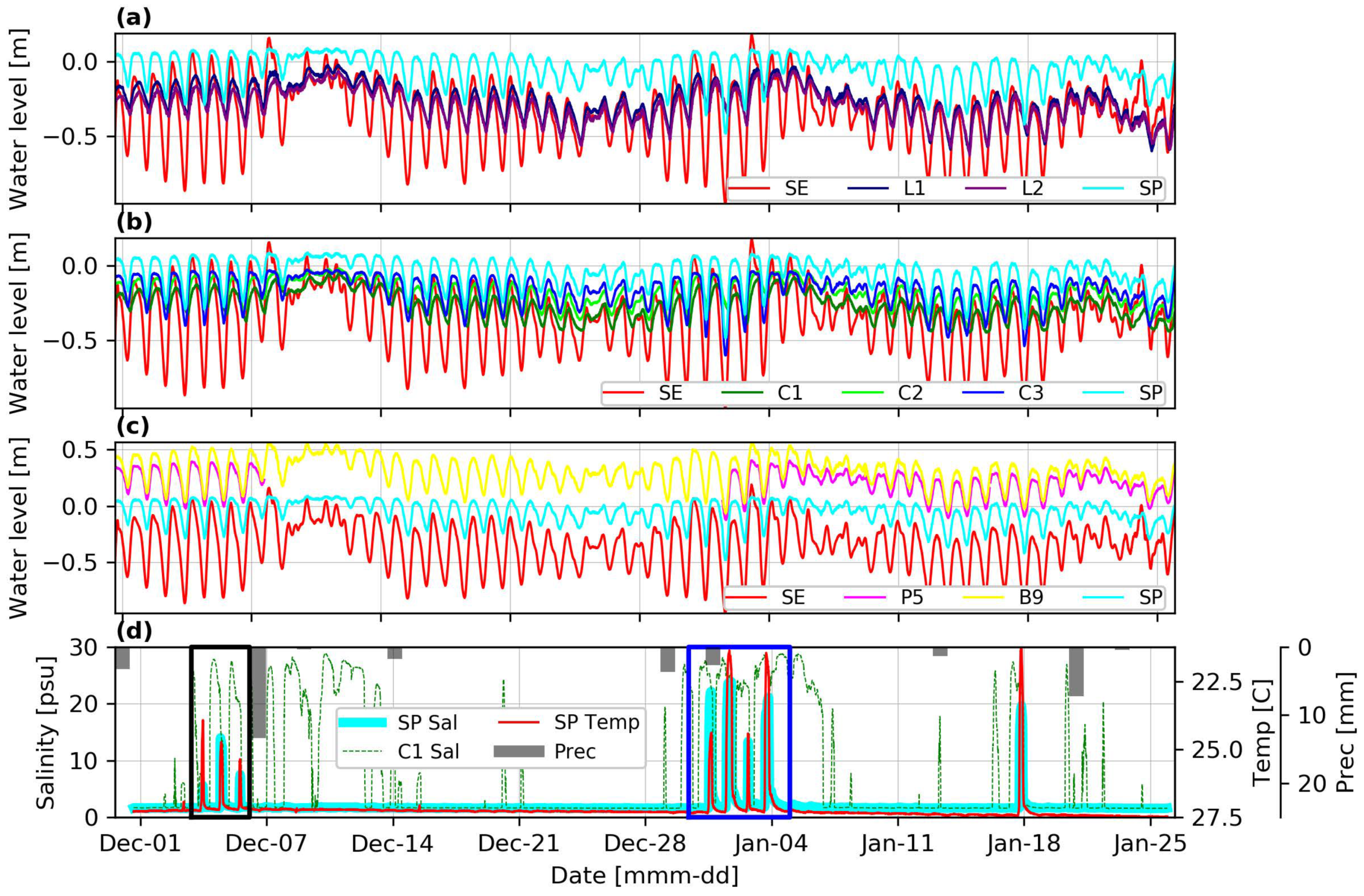
Figure 2 shows the measurements at the stations shown in Figure 1. Figure 2a–c show the water levels in the lagoon, the Peten channel, and the confined aquifer (wells), respectively, which are all compared to the water levels at the spring (SP) and the sea (SE). Figure 2d shows the salinity and temperature at SP, as well as the salinity as C1 (entrance of the Peten channel) as well as the average precipitation on three stations surrounding the study area (Figure 1a). Note that both the temperature and precipitation have their y-values inverted for clarity. From Figure 2d, a total of eight intrusion events are observed, where saltier and colder water from the lagoon reached the spring.
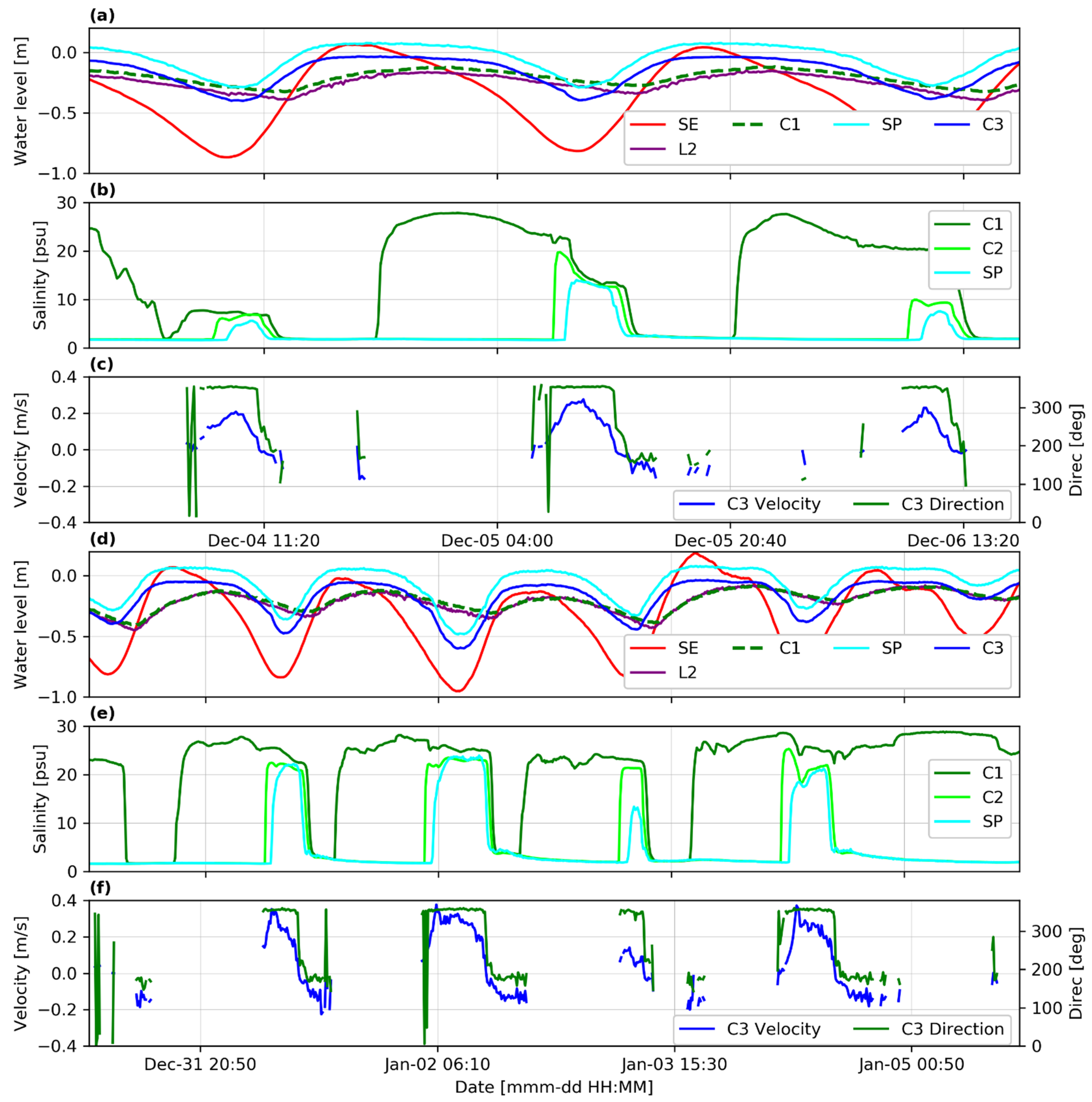
Figure 3 shows a zoom of the two periods with the most intrusion events identified in Figure 2d (black and blue boxes). Water levels at SE, L2, C1, and SP are shown in panels 3a and 3d, salinity measurements at SP, C1, C2 are shown in panels 3b and 3e, and flow velocity and direction at C3 are shown in panels 3c and 3f. The gaps in the velocity record, mainly during outflow from the spring, are due to the lack of enough suspended particles for the signal to be reflected back to the instrument sensors. This does not occur during the salt intrusion events, which allowed the equipment to have good and continuous measurements caused by the debris and suspended particles from the Peten channel.
The intrusion events are the result of the flow reversal in the Peten channel, which is observed from the velocity measurements at C3 (Figure 3c,f): there is a change of about 180° in the direction of the flow during the intrusion, from an average of 175° (spring discharge to the lagoon) to an average of 355° (saline intrusion into the spring), with the maximum measured water velocity during the intrusion events being 0.37 m/s. The intrusion events lasted from 3 to 7 h, with salinity at the spring increasing from 1.6 (groundwater discharge) up to 23.5 psu, and the temperature decreasing from 27.3 to 21.4 °C.
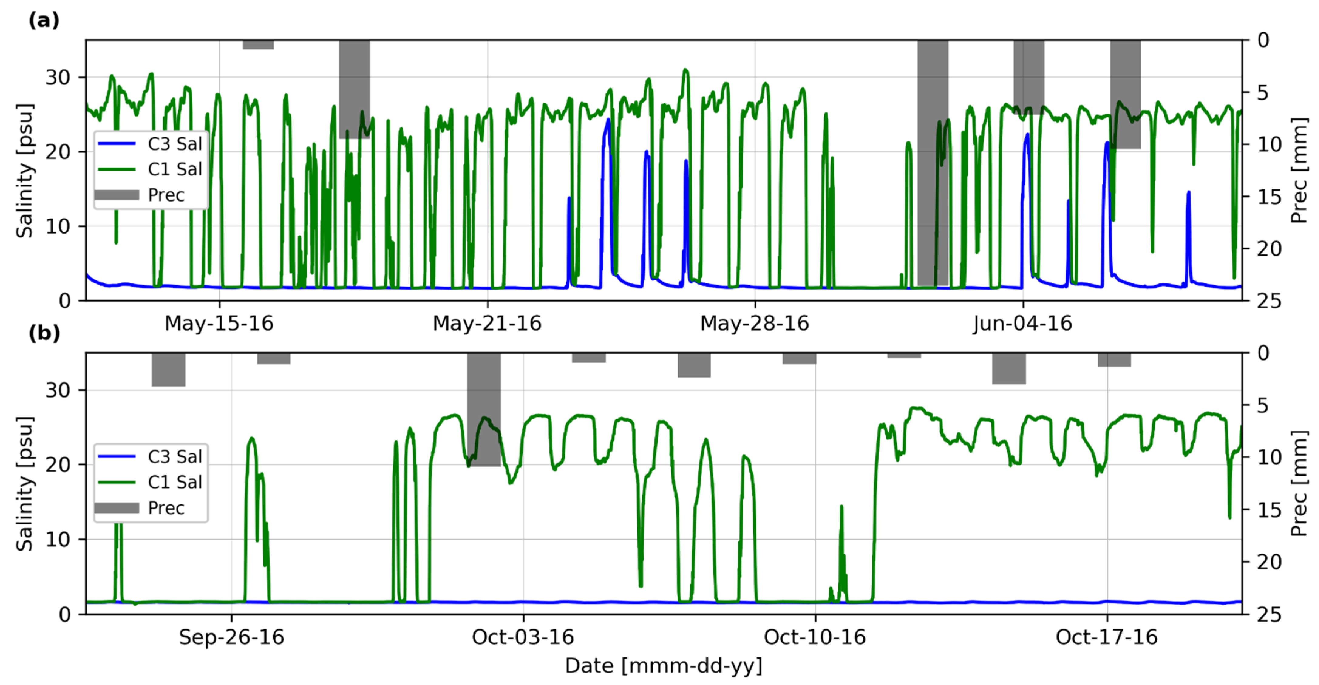
Figure 4a,b show the salinity during two other sampling campaigns to support our discussion about the hydrodynamics of the spring. It is important to mention that for those sampling campaigns, the water levels were not referenced to the same datum, so the data are omitted from this study. Eight saltwater intrusion events are observed in Figure 4b.
Table 1 shows the time lags between SE and the other monitoring stations, which were estimated using cross-correlation analysis [63]. The time lags correspond to the maximum correlation coefficient, which is also shown in the table. Table 2 shows the amplitude of the main tidal components (K1, O1, M2, N2) on the different monitoring stations, their attenuation (ratio between these amplitudes and the amplitude of the same sea component), as well as the phase difference relative to the sea.
3.1. Driving Forces Influencing the Salt Water Intrusion at the Spring
Figure 2d shows the salinity and the temperature on the sensor placed at the opening of the spring (SP, cyan line) and at the entrance of the Peten channel (C1, green dashed line). First, eight strong saltwater intrusion events reaching the spring are observed (the first seven marked with the black and blue boxes): the salinity increases and the temperature decreases as the colder and saltier water from the lagoon enters the Peten channel and eventually intrudes in the spring. There are as well intrusions to the Peten channel that do not reach the spring, as can be seen in the C1 record. Figure 3 shows a zoom of the water levels and salinity during the salt intrusion events (boxes in Figure 2d), as well as flow velocity and direction at C3. It confirms that the saltier lagoon water gets into the channel and in some instances up to the spring during spring low tides (i.e., the lowest monthly tidal level) due to flow reversal as reported by Febles and Batllori [28] and Rey [30], transforming the spring from a source of fresh water to a sink of brackish water. In that sense, this lagoon tidal spring behaves similarly to an estavelle [13].
Figure 3b,e show the salinity at C1 and C2 (entrance and middle section of the Peten channel, respectively) and at SP (spring). At the beginning of ebb, about 40 min (Table 1) after the tide in the sea starts to descend, the head in the spring starts to descend as well, and thus, the discharge of the aquifer decreases, allowing the lagoon brackish water to enter the Peten channel and reach C1. As the aquifer head continues descending, the brackish water advances further up in the channel, mixing with the fresh water, until it reaches the spring (SP). After that, when the tide rises in the ocean, it rises faster in the spring than in the lagoon, increasing the pressure gradient between the spring and the lagoon, which in turn increases the freshwater discharge, decreasing and eventually stopping the saltwater intrusion (Figure S2 in ESM).
For submarine springs in the coastal ocean on the Yucatán Peninsula, salt intrusion and flow reversal may occur at spring high tide [20,26,27]; i.e., when the sea level is higher than the aquifer head, a flow reversal may occur in these springs, which become sinks. Valle-Levinson et al. [20] showed that the flow reversal at the submarine spring is caused by hydraulic pressure gradient and density differences. However, the spring discussed in this work shows an opposite behavior: salt water intrudes at spring low tide. From Table 1 and Table 2, it is clear that the tide is more attenuated and with a higher lag in the lagoon than in the aquifer (spring), suggesting that the confined aquifer responds faster to the tidal signal. This is also observed in Figure 3a,d where the high water is reached later in L2 and C1 than in the stations closer to the spring (C2, C3, and SP). In addition, high (or low) water levels in the ocean (SE, in Figure 3) are expressed rapidly in the spring (SP) with only 40 min time lag (Table 1), while the water levels in the lagoon (L2) and the Peten channel entrance (C1) experience a much larger lag (200 to 210 min). This is confirmed in Table 2, where for each of the main tidal components, the amplitudes decrease (and phases increase) from the sea to C1 due mainly to the high friction in the lagoon, whereas the amplitudes increase (and phases decrease) from C1 to the spring due to the rapid response of the aquifer to tidal changes. Therefore, during spring low tide, the water level in the spring can reach lower values than in the lagoon, producing a pressure gradient-driven flow reversal from the lagoon to the spring (Figure S2 in ESM). However, these pressure gradients are not present in all the intrusion events, in particular those in Figure 3a and the third on Figure 3d (the water level at SP is not lower than at C1), suggesting that the density-driven flow may also play a role. Moreover, the first, second, and fourth flow reversal events shown in Figure 3d are the strongest in terms of salinity at SP, because the combined effect of pressure gradient (or water-level difference) and salinity differences. Indeed, the largest flow reversal event is the second (2 January), in which the water level at the spring is the lowest compared to the water level at C1, and it is also the longest (7 h), which translates in a higher and longer salinity intrusion through the spring. Therefore, the saltwater intrusion in this lagoon tidal spring is caused by density differences and water-level gradients similar to the results of Valle-Levinson [20]. However, even when the main driving forces are the same for this spring and the submarine springs, the intrusion occurs at opposite levels of the tide in the ocean. The main reason for this difference is the existence of the shallow brackish water body between the sea and the spring, which can produce the pressure and density gradients needed for the flow reversal in the spring.
Now, we discuss the mechanisms that influence the density and pressure gradients on the aquifer, lagoon, and Peten channel that may cause the saltwater intrusion.
3.2. Mechanisms Influencing the Driving Forces of Salt Water Intrusion
Tides. Tides are a key component of the dynamics in the coastal aquifer, the lagoon, and Peten channel, as seen in Figure 2 and Figure 3 and Table 1 and Table 2. All the monitoring locations show a tidal behavior, even the wells on the aquifer. This is expected for coastal lagoons and coastal confined aquifers [51,64]. The maximum cross-correlation coefficients (Table 1) between SE and all the monitoring locations are higher than 0.69, and the lags vary from 0 to 210 min. This means that the maximum time that the tide takes to move from the sea to any of the monitoring points is about 210 min (3.5 h at C1). In terms of the individual tidal components, the largest phases with respect to the ocean tide occur at C1, ranging from 3 to 4.4 h, and it is close to 3.5 h for the most energetic components (K1 and O1). As seen before, these phase differences between the spring and the lagoon during spring low tide may produce the pressure gradients that drive the flow reversal and the salt intrusion.
Lagoon bottom friction. The tide signal in the lagoon (L1, L2) is more attenuated, less correlated, and with a greater phase than the signal on the spring and the aquifer, as shown in Table 1 and Table 2. For example, compared with the ocean signal, the K1 amplitudes at L1 and L2 are 37.7% and 33.0% respectively, the correlations are 0.79 and 0.77, and the corresponding phases are 2.63 and 3.34 h, compared to the spring where the corresponding values are 43.7%, 0.94, and 0.81 h. This is mainly due to the high friction in the lagoon being a shallow water body, as reported by Friedrichs et al. [59,65] for shallow estuaries, and the same is true for coastal lagoons [66]. In addition, Tenorio-Fernandez et al. [62] studied another coastal lagoon located next to our study site (La Carbonera) with similar geometric characteristics and concluded that the lagoon is highly frictional, and the hydrodynamics are controlled by a balance between pressure and friction. Given the similitude between La Carbonera and the lagoon studied by Tenorio-Fernandez et al. [62], it is expected for the friction to play an important role in La Carbonera hydrodynamics. Therefore, the bottom friction in the lagoon causes tidal phase lags and amplitude attenuation, which in turn contributes to the generation of the pressure gradients responsible for the flow reversal during spring low tides.
Aquifer confinement. SE and SP water level signals have a strong correlation, as shown in Figure 2a. This is confirmed in Table 1 with a high correlation coefficient of 0.94 and a short lag of 40 min, and in Table 2, where the spring signal shows less attenuation (i.e., higher amplitude) than L1 and L2 and C1. Moreover, the effect of the confinement can also be seen in Figure 2c, where signals of wells P5 and B9 (Figure 1b), located further in land, present a tidal response and also show a strong correlation with the sea and less or similar attenuation than the stations L1 and L2 in the lagoon. This suggest that the water level in the spring pool is highly controlled by the confined aquifer, as reported by [18,36,37], and its interaction with the ocean tide. In fact, White et al. [64] show that the attenuation of the tide in confined aquifers is low and the effects extend more than in unconfined aquifers, which was also found by Canul-Macario et al. [36] and Medina [67] in our study area. On one hand, Canul-Macario et al. [36] report tidal signals in a well in the semiconfined aquifer 12 km from the coast. On the other hand, Medina [67] shows a set of measurements on the unconfined aquifer located in the coastal dune at Sisal beach (Figure 1b), and the tidal signal could not be detected on a well located at 50 m from the coast.
Aquifer recharge and discharge. Figure 4 shows salinity at C1 and C3 and precipitation data from two previous sampling campaigns in 2016: at the end of the dry season (May 2016; panel 4a) when the aquifer recharges, and hence, its discharges through the springs are relatively weak, and at the end of the rainy season (September–October 2016; panel 4b) when the aquifer is fully recharged and the discharges through the springs are strong. On one hand, flow inversions are evident when the aquifer recharge is low (Figure 4a), similar to what occurred in December 2018–January 2019, when the aquifer recharge was also low (Figure 2d). On the other hand, when the aquifer is fully recharged, no salt intrusions occur. This may be the case in Figure 4b, where salinity at C1 (entrance of the Peten channel) is high, but the high aquifer discharge during the rainy season prevented the saltwater intrusion to reach the upper Peten channel and the spring. Regarding the precipitation, Figure 2d and Figure 4 show the average precipitation on stations surrounding our study area, and there is no obvious relationship between the precipitation and the salt intrusions. For instance, precipitation events in June 2016 do not prevent the occurrence of salt intrusions (Figure 4a), suggesting that these events were not strong enough to significantly and rapidly modify the aquifer discharge and prevent the salt intrusions to occur. Furthermore, close to the coast, the aquifer is confined, as reported by [18,36,37], so the recharge in this zone should be less significant than the regional recharge of the aquifer. Given the above, the regional recharge plays a more important role than specific precipitation events on the spring discharge dynamics.
Seasonal and long-term sea-level variations. Zavala-Hidalgo et al. [43] showed the existence of a seasonal variation of the mean sea level, being the lowest during June–August (up to 10 cm below annual mean sea level) and the highest between September and November (up to 15 cm above annual mean sea level) for Progreso, near the study area (see Figure 1a). This cyclic seasonal variation may have an impact on the flow reversal, because it modifies the hydraulic gradients between the sea, the lagoon, and the spring. For instance, Rey [30] reported an inversion event in August 2010, but no inversion is observed in the salinity data shown in Figure 4b (September–October). Both sampling campaigns were carried out during or just after the rainy season (June–September) when the aquifer is recharged; however, the latter campaign occurred when the mean sea level was at its highest annual values (Zavala-Hidalgo et al. 2010). Therefore, the seasonal low mean sea level in August, which translates into lower spring low tides, appears to have promoted the flow inversions reported by Rey [30] in the spring, even though it occurred during the rainy season. Regarding long-term sea level rise due to climate change, Zavala-Hidalgo et al. [43] found the local tendency of sea level rise at Progreso to be of 2.5 ± 1.2 mm per year, while the global scenarios suggested by the International Panel of Climate Change (IPCC) are between 0.4 and 0.7 ± 0.25 m [68,69]. By itself, it has an impact on the lagoon hydrodynamics and the sea–aquifer interaction (e.g., greater salt intrusion), but its effect on the spring flow reversal is not clear.
Spring opening elevation. Given the natural topographic gradient toward the coast, the spring dynamics may also depend on the elevation of the spring opening (in this case, the elevation of the spring pool floor) with respect to the aquifer head and tidal variations. Higher spring opening elevation may translate into lower hydraulic gradient and thus lower freshwater discharge, which in turn could produce stronger and/or more frequent flow reversals at the spring. More data are needed to confirm this possible effect.
Spring pool and Peten channel. Another factor of complexity in the spring dynamics is the elevation of the spring pool margins. In fact, during high tide at the sea, the corresponding high water level at the spring appears flattened (cyan line in Figure 3a,d), which in part is because the pool fills and overflows to the highly frictional surrounding Peten vegetated area. This phenomenon dissipates energy and produces the water level descent at the spring to be slower and less intense, decreasing the negative pressure gradients (between the lagoon and the spring) needed for the flow reversal to occur. Therefore, the spring pool geometry and surrounding topography can affect the flow reversal intensity and frequency. It is important to note that the water level at C3, in Figure 3a,d, is always lower than the water level at SP. The authors claim that this effect may be caused by a flow transition. Mazumder [70] defines a transition as: “Transitions may be broadly defined as that portion of a nonuniform channel undergoing a change in the normal prismatic section. In open channel and closed conduit flows, there are situations when the normal section of flow is to be restricted.” The flow at C3 is subcritical (with an average depth of 1 m, and the maximum measured velocity of 0.37, we obtain a Froude number of 0.11). The flow in the pool is also expected to be subcritical, given its broader section (for this to be proven, more data are required). Therefore, there is a transition from subcritical to subcritical flow. According to Mazumder [70], when a channel is gradually expanded, the discharge intensity decreases, resulting in a rise of the flow depth and vice versa. Therefore, if the flow goes from C3 to SP (expanding channel), the water level would rise, and if the flow goes from SP to C3, the water level would decrease [70].
Wind, storm surges, and local weather. Ref. [29] shows data where the water levels in the lagoon increase as a response to winds. In general, winds can play an important role on the water levels of semi-enclosed water bodies [48,71]. This is not the case in the Peten channel and the spring, given the dense Peten vegetation. Therefore, wind-generated lower (higher) water levels in the lagoon during spring low tide may decrease (increase) the flow reversal frequency and intensity. In the same way, storm surges that affect the mean sea level during several hours or a few days will have an impact on this phenomenon. Canul-Macario et al. [36] showed that the meteorological tides propagate further in the aquifer than astronomical tides. Then, it is expected that if a storm surge occurs during spring low tides, the aquifer head at the spring will increase faster than the lagoon water levels, reducing the pressure gradients needed between the lagoon and the spring for the flow reversal to occur. These potential impacts should be considered in future studies as no strong wind and storm surges occurred during the duration of this study. In addition, local weather (precipitation and evapotranspiration) in the lagoon and surrounding areas may decrease or increase the lagoon water salinity and have an impact on the density-driven flows in the Peten channel, affecting the frequency and intensity of the inversion events. No strong precipitation events in the area occurred during or just before the spring low tides analyzed in this study.
4. Conclusions
The hydrodynamics of a lagoon tidal spring on a northern Yucatán coast is analyzed. Measurements of water levels, salinity, temperature, and flow velocity confirm the occurrence of saltwater intrusion events from the lagoon to the underlying confined aquifer through the spring. The intrusion events occur during spring low tides, opposite to inversion events in nearby submarine springs on the coastal ocean floor. The forcings controlling the inversion events are similar for submarine and lagoon springs on the northern Yucatán coast: pressure and density gradients. However, the fact that there is a semi-enclosed shallow water body between the spring and the sea plays a central role on the saltwater intrusion dynamics.
Using cross-correlation analysis and tidal harmonic decomposition on all measured data, the main driving forces of the saltwater intrusion events are found to be density and pressure gradients. This is concluded from the fact that at some intrusion events, there is a pressure gradient between the lagoon and the spring, and for the other events, there is no pressure gradient, but still brackish water gets into the spring. Thus, density and pressure gradients should play a key role. The main driving forces are further addressed by discussing different involved mechanisms and its influence. For example, the tides are central to the discussed dynamics given that the signal is present in all the measuring sites. In addition, there are density gradients caused by the density of the fresh water of the spring and the sea. The tide signal is delayed on the lagoon when compared to the wells; thus, the high friction of the lagoon should also play a central role for the salt intrusion events to occur. In addition, the natural variation of the mean sea level and the wet/dry season head in the aquifer through the year may influence the dynamics. For example, no intrusion events are observed during the recharge season of the aquifer. Other factors such as the spring pool, spring opening elevation, and local weather can also have an effect on the spring/lagoon interaction.
The authors claim that the data collected and presented are enough to support the conclusions of the present work about the dynamics of this spring. However, we recognize that additional studies are required to further understand the complex dynamics of the salt intrusion events. For example, measurements during a complete year would help to understand the behavior of the events during different seasons. In addition to the salinity and water level measurements, hydrochemistry as well as water isotope measurements could provide evidence about the involved processes and confirm the importance of the proposed mechanisms.
A better understanding of such saltwater intrusion events is important for coastal management, especially in these dynamic ecosystems, which are threatened by climate change and can affect coastal freshwater availability.
Supplementary Materials
The following are available online at https://www.mdpi.com/article/10.3390/w13233431/s1, Figure S1: Elevations of points along the Peten channel bottom. The elevation was measured at the middle section approximately. The red squares show the location of the three measurements sites (C1, C2, and C3); Figure S2: Water levels, salinity measurements at SE, C1, C3, and SP, and the hydraulic gradient between SE, C1, C3, and SP.
Author Contributions
Conceptualization, R.P.-C. and P.S.; methodology, C.C.-M. and A.P.-H.; software, R.P.-C.; formal analysis, R.P.-C. and P.S.; investigation, R.P.-C., C.C.-M. and P.S.; data curation R.P.-C., C.C.-M. and A.P.-H.; writing—original draft preparation, R.P.-C.; writing—review and editing, R.P.-C., P.S., C.C.-M. and A.P.-H.; visualization, R.P.-C.; supervision, P.S.; project administration, P.S.; funding acquisition, P.S. All authors have read and agreed to the published version of the manuscript.
Funding
R.P.-C. is a CONACyT research fellow commissioned to the Universidad Nacional Autónoma de México through the Cátedras Program (No. 1146). Additional financial support was provided by the National Coastal Resilience Laboratory (LANRESC) through projects No. 299063 and No. 315908.
Institutional Review Board Statement
Not applicable.
Informed Consent Statement
Not applicable.
Data Availability Statement
The precipitation data presented are openly available in https://www.ruoa.unam.mx/ (accessed on 4 July 2021). The data presented in this study are available on request from the corresponding author.
Acknowledgments
R.P.-C. (Roger Pacheco-Castro) thanks to Catedras-CONACyT for the funding as research fellow commissioned to the Universidad Nacional Autónoma de México. The authors thank the support of the National Coastal Resilience Laboratory for funding for this project. Field support was provided by José López González and Juan Gomez Liera. IT technical support was provided Gonzalo Uriel Martín Ruiz. The authors thank the “Red Universitaria de Observatorios Atmosféricos de la Universidad Nacional Autónoma de México” for the precipitation data.
Conflicts of Interest
The authors declare no conflict of interest.
References
- Ford, D.; Williams, P. Karst Hydrogeology and Geomorphology; John Wiley & Sons Ltd.: West Sussex, UK, 2007; ISBN 9781118684986. [Google Scholar]
- Groves, C. Methods in Karst Hydrogeology; Goldscheider, N., Drew, D., Eds.; Taylor and Francis Group: London, UK, 2007; ISBN 9780415428736. [Google Scholar]
- Kresic, N.; Stevanovic, Z. Groundwater and Hydrology in Springs; Kresic, N., Stevanovic, Z., Eds.; Elsevier: Amsterdam, The Netherlands, 2010; p. 567. ISBN 9781856175029. [Google Scholar]
- COSOD II. Report of the Second Conference on Scientific Ocean Drilling COSOD II; European Science Foundation: Strassbourg, France, 1987; p. 154. ISBN 2-903148-52-X. [Google Scholar]
- Karanjac, J.; Gunay, G. Dumanli Spring, Turkey—The largest karstic spring in the world? J. Hydrol. 1980, 45, 219–231. [Google Scholar] [CrossRef]
- Scott, T.M.; Means, G.H.; Means, R.C.; Meegan, R.P. First Magnitude Springs of Florida; Florida Geological Survey: Tallahassee, FL, USA, 2002.
- Scott, T.; Means, G.; Rebecca, M.; Means, R.; Upchurch, S.; Copeland, R.E.; Jones, J.; Roberts, T.; Willet, A. Springs of Florida; Florida Geological Survey: Tallahassee, FL, USA, 2004.
- Kresic, N. Foreword: Ground water in karst. Ground Water 2009, 47, 319–320. [Google Scholar] [CrossRef]
- Springer, A.E.; Stevens, L.E. Spheres of discharge of springs. Hydrogeol. J. 2009, 17, 83–93. [Google Scholar] [CrossRef]
- Taniguchi, M.; Burnett, W.C.; Cable, J.E.; Turner, J.V. Investigation of submarine groundwater discharge. Hydrol. Process. 2002, 16, 2115–2129. [Google Scholar] [CrossRef]
- UNESCO. Submarine Groundwater Discharge; United Naions Educational, Scientific and Cultural Organization: Paris, France, 2014; ISBN 9780128130810. [Google Scholar]
- Vineyard, J.; Feder, G. Springs of Missouri; Missouri Department of Natural Resources: Jefferson City, MO, USA, 1982.
- Bogli, A. Karst Hydrology and Physical Speleology; Springer: Amsterdam, The Netherlands, 1980; ISBN 0387100989. [Google Scholar]
- Batllori Sampedro, E.; González Piedra, J.I.; Díaz Sosa, J.; Febles Patrón, J.L. Caracterización hidrológica de la región costera noroccidental del estado de yucatán, México. Investig. Geogr. 2006, 59, 74–92. (In Spanish) [Google Scholar] [CrossRef]
- Rey, W. Evaluación del Peligro a la Inundación Inducida por Eventos Extremos de Tormenta en el Norte de la Península de Yucatán; Universidad Autónoma de Yucatán: Mérida, México, 2017; p. 121. (In Spanish) [Google Scholar]
- Lane, E. The Spring Creek Submarine Springs Group, Wakulla County, Florida; Florida Geological Survey: Tallahassee, FL, USA, 2001.
- Davis, J.H.; Verdi, R. Groundwater flow cycling between a submarine spring and an inland fresh water spring. Ground Water 2014, 52, 705–716. [Google Scholar] [CrossRef] [PubMed]
- Perry, E. Geologic and environmental aspects of surface cementation, north coast, Yucatan, Mexico. Geology 1989, 17, 818–821. [Google Scholar] [CrossRef]
- Bonacci, O.; Bojanic, D. Rhytmic karst springs. Hydrol. Sci. J. 1991, 36, 35–47. [Google Scholar] [CrossRef]
- Valle-Levinson, A.; Mariño-Tapia, I.; Enriquez, C.; Waterhouse, A.F. Tidal variability of salinity and velocity fields related to intense point-source submarine groundwater discharges into the Coastal Ocean. Limnol. Oceanogr. 2011, 56, 1213–1224. [Google Scholar] [CrossRef]
- Williams, P.W. Hydrogeology of the Waikouropupu springs: A major tidal karst resurgence in northwest Nelson (New Zealand). J. Hydrol. 1977, 35, 73–92. [Google Scholar] [CrossRef]
- McCormack, T.; Gill, L.W.; Naughton, O.; Johnston, P.M. Quantification of submarine/intertidal groundwater discharge and nutrient loading from a lowland karst catchment. J. Hydrol. 2014, 519, 2318–2330. [Google Scholar] [CrossRef]
- Schuler, P.; Duran, L.; McCormack, T.; Gill, L. Submarine and intertidal groundwater discharge through a complex multi-level karst conduit aquifer. Hydrogeol. J. 2018, 26, 2629–2647. [Google Scholar] [CrossRef] [Green Version]
- Holliday, D.; Stieglitz, T.C.; Ridd, P.V.; Read, W.W. Geological controls and tidal forcing of submarine groundwater discharge from a confined aquifer in a coastal sand dune system. J. Geophys. Res. Oceans 2007, 112. [Google Scholar] [CrossRef] [Green Version]
- Fleury, P.; Bakalowicz, M.; de Marsily, G. Submarine springs and coastal karst aquifers: A review. J. Hydrol. 2007, 339, 79–92. [Google Scholar] [CrossRef]
- Parra, S.M.; Valle-Levinson, A.; Mariño-Tapia, I.; Enriquez, C. Salt intrusion at a submarine spring in a fringing reef lagoon. J. Geophys. Res. Oceans 2015, 120, 2736–2750. [Google Scholar] [CrossRef]
- Parra, S.M.; Valle-Levinson, A.; Mariño-Tapia, I.; Enriquez, C.; Candela, J.; Sheinbaum, J. Seasonal variability of saltwater intrusion at a point-source submarine groundwater discharge. Limnol. Oceanogr. 2016, 61, 1245–1258. [Google Scholar] [CrossRef]
- Febles, J.; Batllori, E. Fluctuación diurna del nivel hidrostático en petenes de la cuenca costera noroccidental del estado de Yucatán: Efecto del desazolve y la canalización de manantiales. Tecnol. Cienc. Agua 1995, 10, 5–19. (In Spanish) [Google Scholar]
- Marin, E. Modelación de la Hidrodinámica de un Sistema Lagunar en Humedal Costero con Descargas de Agua Subterránea (DAS) y su Relación con la Distribución de Algunas Especies de Icitofauna; Universidad Nacional Autónoma De México: Mexico City, Mexico, 2016. (In Spanish) [Google Scholar]
- Rey, W. Evaluación Hidrodinámica y Modelación Numérica de la Laguna la Carbonera, Yucatán; Universidad Autónoma de Yucatán: Yucatán, Mexico, 2012. (In Spanish) [Google Scholar]
- Back, W. The Yucatan Peninsula, Mexico. In Karst Hydrogeology and Human Activities: Impacts, Consequences and Implications: IAH International Contributions to Hydrogeology 20; IAH—International Contributions to Hydrogeology; Drew, D., Hötzl, H., Eds.; CRC Press: Boca Raton, FL, USA, 1999; pp. 14–19. ISBN 978-90-5410-464-3. [Google Scholar]
- Doehring, D.; Butler, J. Hydrogeologic constraints on Yucatan’s development. Sci. Am. Assoc. Adv. Sci. 1987, 186, 591–595. [Google Scholar]
- INEGI. Estudio Hidrológico del Estado de Yucatán; Instituto Nacional de Estadística, Geografía e Informática: Aguascalientes, Mexico, 2002. (In Spanish) [Google Scholar]
- Villasuso, M.; Méndez, R. A conceptual model of the Aquifer of the Yucatán Peninsula. In Population, Development, and Environment on the Yucatan Peninsula: From Ancient Maya to 2030; Lutz, W., Prieto, L., Sanderson, W., Eds.; IIASA: Laxenburg, Austria, 2000; pp. 120–139. ISBN 3-7045-0138-7. [Google Scholar]
- SGM; INEGI. Carta Geologico-Minera Tizimin F16-7; Servicio Geológico Mexicano: Pachuca, Mexico, 2006. (In Spanish)
- Canul-Macario, C.; Salles, P.; Hernández-Espriú, A.; Pacheco-Castro, R. Empirical relationships of groundwater head–salinity response to variations of sea level and vertical recharge in coastal confined karst aquifers. Hydrogeol. J. 2020, 28, 1679–1694. [Google Scholar] [CrossRef]
- Pino, M.J.V.; Y Pinto, I.A.S.; Macario, C.C.; Salazar, R.C.; Escobedo, G.B.; Cetina, J.S.; Euán, P.P.; Argüelles, C.P. Hydrogeology and conceptual model of the karstic coastal aquifer in Northern Yucatan State, Mexico. Trop. Subtrop. Agroecosyst. 2011, 13, 243–260. [Google Scholar]
- Perry, E.; Velazquez-Oliman, G.; Marin, L. The hydrogeochemistry of the karst aquifer system of the northern yucatan peninsula, Mexico. Int. Geol. Rev. 2002, 44, 191–221. [Google Scholar] [CrossRef]
- Escolero, O.; Marin, L.; Steinich, B.; Pacheco, J. Delimitation of a hydrogeological reserve for a city within a karstic aquifer: The Merida, Yucatan example. Landsc. Urban Plan. 2000, 51, 53–62. [Google Scholar] [CrossRef]
- Marín, L.E.; Steinich, B.; Pacheco, J.; Escolero, O.A. Hydrogeology of a contaminated sole-source karst aquifer, Mérida, Yucatán, Mexico. Geofis. Int. 2000, 39, 359–365. [Google Scholar] [CrossRef]
- Pacheco, A.J.; Cabrera, S.A. Groundwater contamination by nitrates in the Yucatan Peninsula, Mexico. Hydrogeol. J. 1997, 5, 47–53. [Google Scholar] [CrossRef]
- Pacheco, J.; Marín, L.; Cabrera, A.; Steinich, B.; Escolero, O. Nitrate temporal and spatial patterns in 12 water-supply wells, Yucatan, Mexico. Environ. Geol. 2001, 40, 708–715. [Google Scholar] [CrossRef]
- Zavala, J.; de Buen, R.; Romero, R.; Hernández, F. Tendencias del nivel del mar en las costas mexicanas. In Vulnerabilidad de las Zonas Costeras Mexicanas ante el Cambio Climático; Botello, A.V., Villanueva-Fragoso, S., Gutiérrez, J., Rojas Galaviz, J.L., Eds.; Gobierno del Estado de Tabasco: Villahermosa, Mexico, 2011. (In Spanish) [Google Scholar]
- Goujon, A.; Kohler, I.; Lutz, W. Future population and education trends: Scenarios to 2030 by socioecological region. In Population, Development, and Environment on the Yucatán Peninsula: From Ancient Maya to 2030; Lutz, W., Prieto, L., Sanderson, W., Eds.; International Institute for Applied Systems Analysis: Luxemburg, Austria, 2000. [Google Scholar]
- Herrera-Silveira, J.A.; Morales-Ojeda, S.M. Evaluation of the health status of a coastal ecosystem in southeast Mexico: Assessment of water quality, phytoplankton and submerged aquatic vegetation. Mar. Pollut. Bull. 2009, 59, 72–86. [Google Scholar] [CrossRef]
- García, A.; Xool, M.; Euán, J.; Munguía, A.; Cervera, M. La Costa de Yucatán En La Perspectiva Del Desarrollo Turístico Del Desarrollo Turístico; CONABIO, Ed.; SEMARNAT-CONABIO: Mexico City, Mexico, 2011; ISBN 9786077607441. (In Spanish) [Google Scholar]
- Ketabchi, H.; Mahmoodzadeh, D.; Ataie-Ashtiani, B.; Simmons, C.T. Sea-level rise impacts on seawater intrusion in coastal aquifers: Review and integration. J. Hydrol. 2016, 535, 235–255. [Google Scholar] [CrossRef]
- Lankford, R. Coastal lagoons of Mexico their origin and classification. In Estuarine Processes; Wiley, M., Ed.; Academic Press: Cambridge, MA, USA, 1977. [Google Scholar]
- Mariño-Tapia, I.; Enriquez, C.; Medellin, G.; González, M.; Uc, E.; Medina, I. Estudios Batimétricos, Hidrodinámicos y de Calidad de Agua de Lagunas Costeras de Yucatán; Centro de Investigación y de Estudios Avanzados del Instituto Politécnico Nacional, Unidad Mérida: Merida, México, 2011. (In Spanish) [Google Scholar]
- Bonilla-Gómez, J.L. Environmental Influences on the Abundance of Dominant Fishes in a Very Shallow Tropical Coastal Lagoon in Northwestern Yucatan Peninsula, Mexico. J. Mar. Sci. Res. Dev. 2013, 3, 1–11. [Google Scholar] [CrossRef]
- Kjerfve, B. Coastal lagoons. In Coastal Lagoon Processes; Kjerfve, B., Ed.; Elsevier Oceanography Series: Amsterdam, The Netherlands, 1994; pp. 1–8. [Google Scholar]
- Luis Bonilla-Gómez, J.; Badillo-Alemán, M.; Gallardo-Torres, A.; Chiappa-Carrara, X. Temporal Variation, Growth and Natural Mortality of Two Species of Mojarras (Perciformes: Gerreidae). Rev. Mar. Cost. 2013, 5, 57–67. [Google Scholar] [CrossRef]
- Servicio Geologico Mexicano Cartografía Geológica de la República Mexicana Escala 1:250,000. Available online: https://datos.gob.mx/busca/dataset/cartografia-geologica-de-la-republica-mexicana-escala-1-250000/resource/ae3cf07d-b7e7-4efa-a5ab-faba976a1c1f (accessed on 7 April 2021). (In Spanish).
- Lewis, E.L. The Practical Salinity Scale 1978 and Its Antecedents. Mar. Geod. 1980, 5, 351–357. [Google Scholar] [CrossRef]
- McDougall, T.J.; Barker, P.M. Getting started with TEOS-10 and the Gibbs Seawater (GSW) Oceanographic Toolbox. Scor/Iapso WG 2011, 127, 1–28. [Google Scholar]
- Universidad Nacional Autónoma de México Red Universitaria de Observatorios Atmosféricos de la Universidad Nacional Autónoma de México. Available online: https://www.ruoa.unam.mx/ (accessed on 4 July 2021). (In Spanish).
- Ferris, J.G. Cyclic Fluctuations of Water Level as a Basis for Determining Aquifer Transmissibility; United States Department of the Interior Geological Survey, Water Resources Division, Groundwater Branch: Washington, DC, USA, 1952.
- Kjerfve, B. Tides of the Caribbean Sea. J. Geophys. Res. 1981, 86, 4243–4247. [Google Scholar] [CrossRef]
- Friedrichs, C.T.; Madsen, O.S. Nonlinear diffusion of the tidal signal in frictionally dominated embayments. J. Geophys. Res. 1992, 97, 5637. [Google Scholar] [CrossRef]
- Pawlowicz, R.; Beardsley, B.; Lentz, S. Classical tidal harmic analysis including error estimates in MATLAB and T_Tide. Comput. Geosci. 2002, 28, 929–937. [Google Scholar] [CrossRef]
- Boon, J.D. Secrets of the Tide: Tide and Tidal Current Analysis and Predictions, Storm Surges and Sea Level Trends; Woodhead Publishing Limited: Sawston, UK, 2004; ISBN 9781904275176. [Google Scholar]
- Tenorio-Fernandez, L.; Gomez-Valdes, J.; Marino-Tapia, I.; Enriquez, C.; Valle-Levinson, A.; Parra, S.M. Tidal dynamics in a frictionally dominated tropical lagoon. Cont. Shelf Res. 2016, 114, 16–28. [Google Scholar] [CrossRef]
- Chatfield, C.; Xing, H. The Analysis of Time Series: An Introduction with R, 7th ed.; CRC Press: Boca Raton, FL, USA, 2019. [Google Scholar]
- White, J.K.; Roberts, T.O.L. 2. The significance of groundwater tidal fluctuations. In Groundwater Problems in Urban Areas; Springer: Amsterdam, The Netherlands, 1994. [Google Scholar]
- Friedrichs, C. Baroclinic tides in channelized estuaries. In Contemporary Issues in Estuarine Physics; Valle-Levinson, A., Ed.; Cambridge University Press: Cambridge, MA, USA, 2010; pp. 27–61. [Google Scholar]
- Spaulding, M.L. Modeling of Circulation and Dispersion in Coastal Lagoons; Kjerfve, B., Ed.; Elsevier Science Publishers: Amsterdam, The Netherlands, 1994. [Google Scholar]
- Medina-Rosado, J.A. Caracterización Geohidrológica del Acuífero de la Duna Costera de Sisal, Yucatán; Universidad Autónoma de Yucatán: Yucatán, Mexico, 2020. [Google Scholar]
- Church, J.A.; Clark, P.U.; Cazenave, A.; Gregory, J.; Jevrejava, S.; Lebermann, A.; Merrifield, M.; Milne, G.; Nerem, R.S.; Nunn, P.; et al. Sea Level Change. In Climate Change 2013: The Physical Science Basis. Contribution of Working Group I to the Fifth Assessment Report of the Intergovernmental Panel on Climate Change; Jouzel, J., van de Wal, R., Woodworth, P., Xiao, C., Eds.; Cambridge University Press: New York, NY, USA, 2013; p. 227. [Google Scholar]
- IPCC. Summary for Policymakers; Masson-Delmotte, V., Zhai, P., Pörtner, H.-O., Roberts, D., Skea, J., Shukla, P.R., Pirani, A., Moufouma-Okia, W., Péan, C., Pidcock, R., et al., Eds.; Springer: Cham, Switzerland, 2018. [Google Scholar]
- Mazumder, S.K. Flow Transition Design in Hydraulic Structures; CRC Press: Boca Raton, FL, USA, 2020. [Google Scholar]
- Winant, C. Wind and tidally driven flows in a semienclosed basin. Contemp. Issues Estuar. Phys. 2010, 125–144. [Google Scholar] [CrossRef]
Figure 2.
Data from sites shown in Figure 1, collected in 2017–2018: (a) Water levels in the lagoon (L1, L2), SE, and SP. (b) Water levels in the Peten channel (C1, C2, C3), SP, and SE. (c) Water levels at SE and SP and hydraulic head at wells B9 and P5. All the water levels are referenced to the same datum. (d) Water salinity and temperature at SP and average daily precipitation in the study zone. The black and blue squares show the salt intrusions zoomed in Figure 3.

Figure 3.
Zoom to the salt intrusion inversion events shown in the black (panels (a–c)) and blue (panels (d–f)) boxes of Figure 2d. (a,d) Water levels in the spring (SP), sea (SE), and lagoon entrance and end of the Peten Channel (C1, C3). (b,e) Salinity in the Peten channel (C1 and C2) and spring. (d,f) Flow velocity and direction at near the spring pool (C3); positive (negative) velocity values correspond to brackish (freshwater) inflow into the spring (outflow).

Figure 4.
Salinity measurements in the Peten channel (C1 and C3) and average precipitation: (a) May–June 2016, (b) September–October 2016.
Figure 4.
Salinity measurements in the Peten channel (C1 and C3) and average precipitation: (a) May–June 2016, (b) September–October 2016.


Table 1.
Maximum cross-correlation and lag values between SE and the other monitoring points. The lag is where the maximum cross-correlation value occurs.
Table 1.
Maximum cross-correlation and lag values between SE and the other monitoring points. The lag is where the maximum cross-correlation value occurs.
| Lagoon | Channel | Aquifer | |||||
|---|---|---|---|---|---|---|---|
| L1 | L2 | C1 | C2 | C3 | SP | B9 | |
| lag (min) | 150 | 200 | 210 | 130 | 40 | 40 | 30 |
| r | 0.79 | 0.77 | 0.76 | 0.83 | 0.94 | 0.94 | 0.96 |
Table 2.
Main tidal components amplitude on the sea (SE), lagoon (L1, L2), Peten channel (C1, C2, C3), spring (SP), and aquifer wells. The ratios and phases at each station and for each component are relative to the sea tide.
Table 2.
Main tidal components amplitude on the sea (SE), lagoon (L1, L2), Peten channel (C1, C2, C3), spring (SP), and aquifer wells. The ratios and phases at each station and for each component are relative to the sea tide.
| Component | Sea | Lagoon | Channel and Spring | Aquifer | |||||
|---|---|---|---|---|---|---|---|---|---|
| SE | L1 | L2 | C1 | C2 | C3 | SP | B9 | ||
| K1 | Amp. (m) | 0.2218 | 0.0837 | 0.0732 | 0.0611 | 0.0698 | 0.0963 | 0.0970 | 0.1201 |
| Ratio | 100% | 37.7% | 33.0% | 27.5% | 31.5% | 43.4% | 43.7% | 54.1% | |
| Phase (h) | 0 | 2.63 | 3.34 | 3.35 | 2.20 | 0.83 | 0.81 | 0.57 | |
| O1 | Amp. (m) | 0.1696 | 0.0575 | 0.0500 | 0.0403 | 0.0501 | 0.0772 | 0.0774 | 0.0948 |
| Ratio | 100% | 33.9% | 29.5% | 23.8% | 29.5% | 45.5% | 45.6% | 55.9% | |
| Phase (h) | 0 | 2.61 | 3.47 | 3.84 | 2.43 | 1.02 | 0.99 | 0.68 | |
| M2 | Amp. (m) | 0.0674 | 0.019 | 0.0153 | 0.0102 | 0.0141 | 0.0323 | 0.0324 | 0.0344 |
| Ratio | 100% | 28.2% | 22.7% | 15.1% | 20.9% | 47.9% | 48.1% | 51.0% | |
| Phase (h) | 0 | 2.0 | 2.7 | 3.0 | 1.2 | 0.0 | 0.0 | 0.2 | |
| N2 | Amp. (m) | 0.025 | 0.0052 | 0.0044 | 0.004 | 0.0051 | 0.0109 | 0.0109 | 0.0123 |
| Ratio | 100% | 20.8% | 17.6% | 16.0% | 20.4% | 43.6% | 43.6% | 49.2% | |
| Phase (h) | 0 | 2.9 | 3.4 | 4.4 | 2.1 | 0.5 | 0.5 | 0.4 | |
Publisher’s Note: MDPI stays neutral with regard to jurisdictional claims in published maps and institutional affiliations. |
© 2021 by the authors. Licensee MDPI, Basel, Switzerland. This article is an open access article distributed under the terms and conditions of the Creative Commons Attribution (CC BY) license (https://creativecommons.org/licenses/by/4.0/).
Share and Cite
MDPI and ACS Style
Pacheco-Castro, R.; Salles, P.; Canul-Macario, C.; Paladio-Hernandez, A. On the Understanding of the Hydrodynamics and the Causes of Saltwater Intrusion on Lagoon Tidal Springs. Water 2021, 13, 3431. https://doi.org/10.3390/w13233431
AMA Style
Pacheco-Castro R, Salles P, Canul-Macario C, Paladio-Hernandez A. On the Understanding of the Hydrodynamics and the Causes of Saltwater Intrusion on Lagoon Tidal Springs. Water. 2021; 13(23):3431. https://doi.org/10.3390/w13233431
Chicago/Turabian StylePacheco-Castro, Roger, Paulo Salles, Cesar Canul-Macario, and Alejandro Paladio-Hernandez. 2021. "On the Understanding of the Hydrodynamics and the Causes of Saltwater Intrusion on Lagoon Tidal Springs" Water 13, no. 23: 3431. https://doi.org/10.3390/w13233431
Note that from the first issue of 2016, this journal uses article numbers instead of page numbers. See further details here.