
Natural Background Levels of Potentially Toxic Elements in Groundwater from a Former Asbestos Mine in Serpentinite (Balangero, North Italy)

 , and
, and
Abstract
:1. Introduction
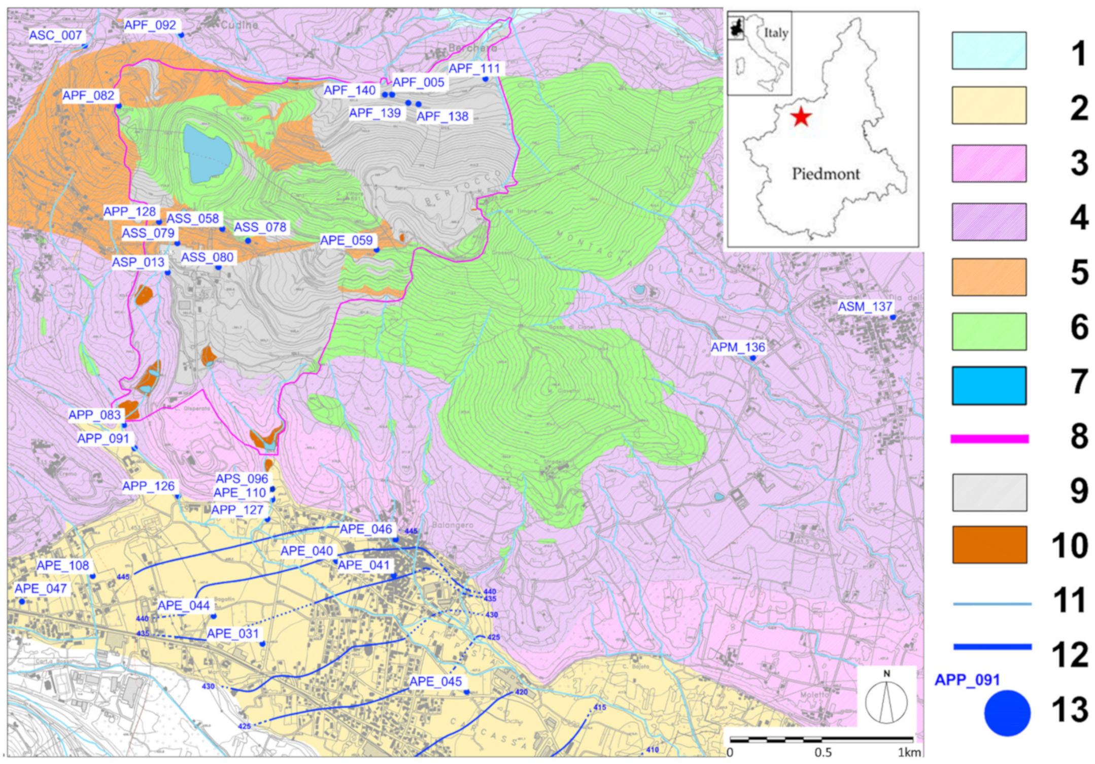
2. Study Area

Hydrogeology
- the crystalline rocks of the Sesia–Lanzo zone (henceforth indicated as SL);
- the serpentinite of the Lanzo Massif (henceforth indicated as SERP);
- the fluvial deposits, the glacial basal and ablation deposits of Middle Pleistocene, the fluvial deposits of Lower Pleistocene (grouped together as fluvioglacial deposits) and their colluvial–eluvial covers (henceforth indicated as FGD);
- the alluvial deposits constituting the Balangero Plain (henceforth indicated as BPA).
3. Materials and Methods
3.1. The Italian Legislative Framework
3.2. Sampling and Analytical Methods
3.3. Data Validation and Selection
4. Results
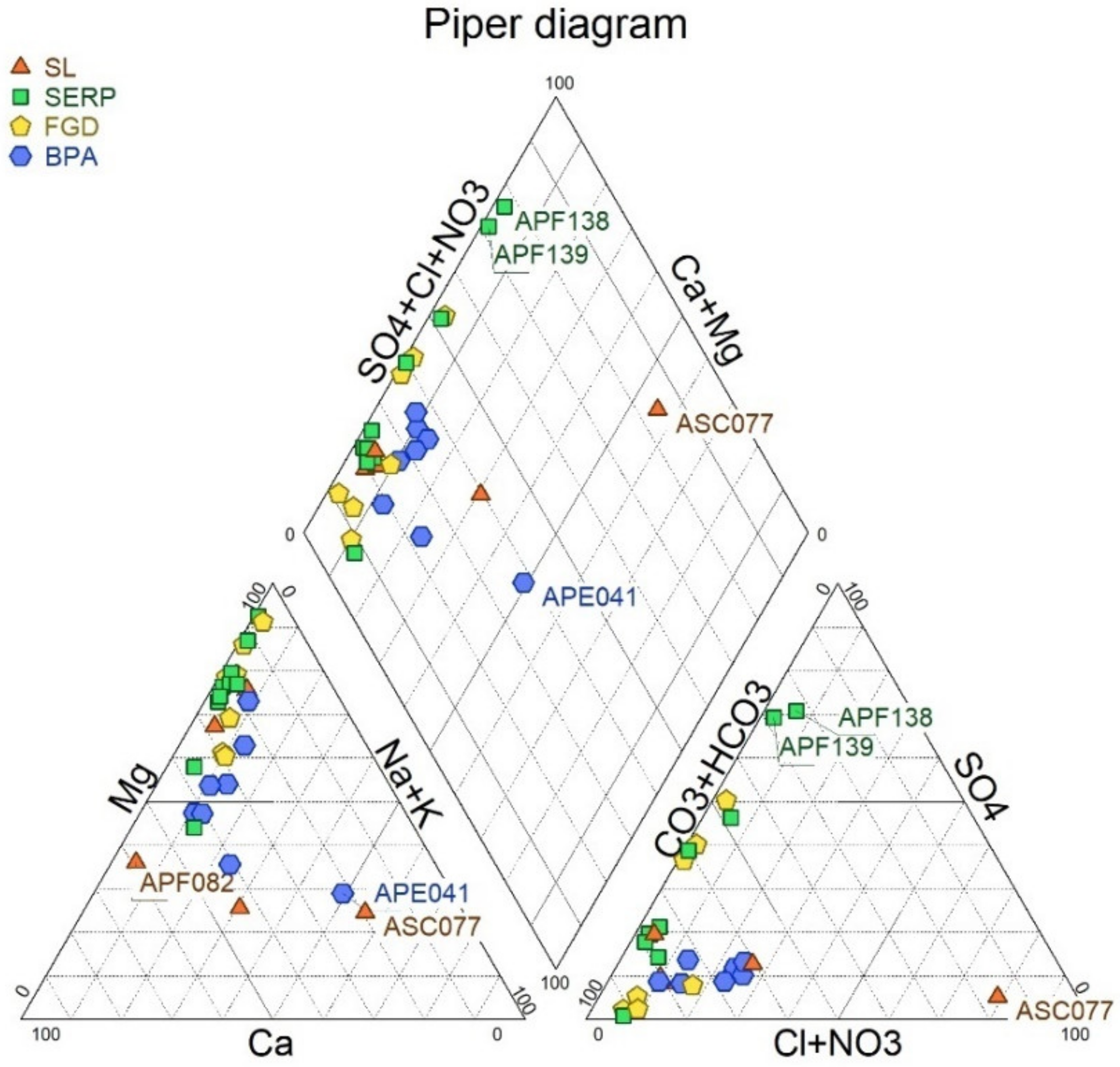
4.1. Hydrochemical Facies
4.2. Pre-Selection
5. Data Treatment
5.1. Trend Analysis
5.2. Spatial Analysis
5.2.1. Total and Hexavalent Chromium
5.2.2. Nickel
5.2.3. Manganese
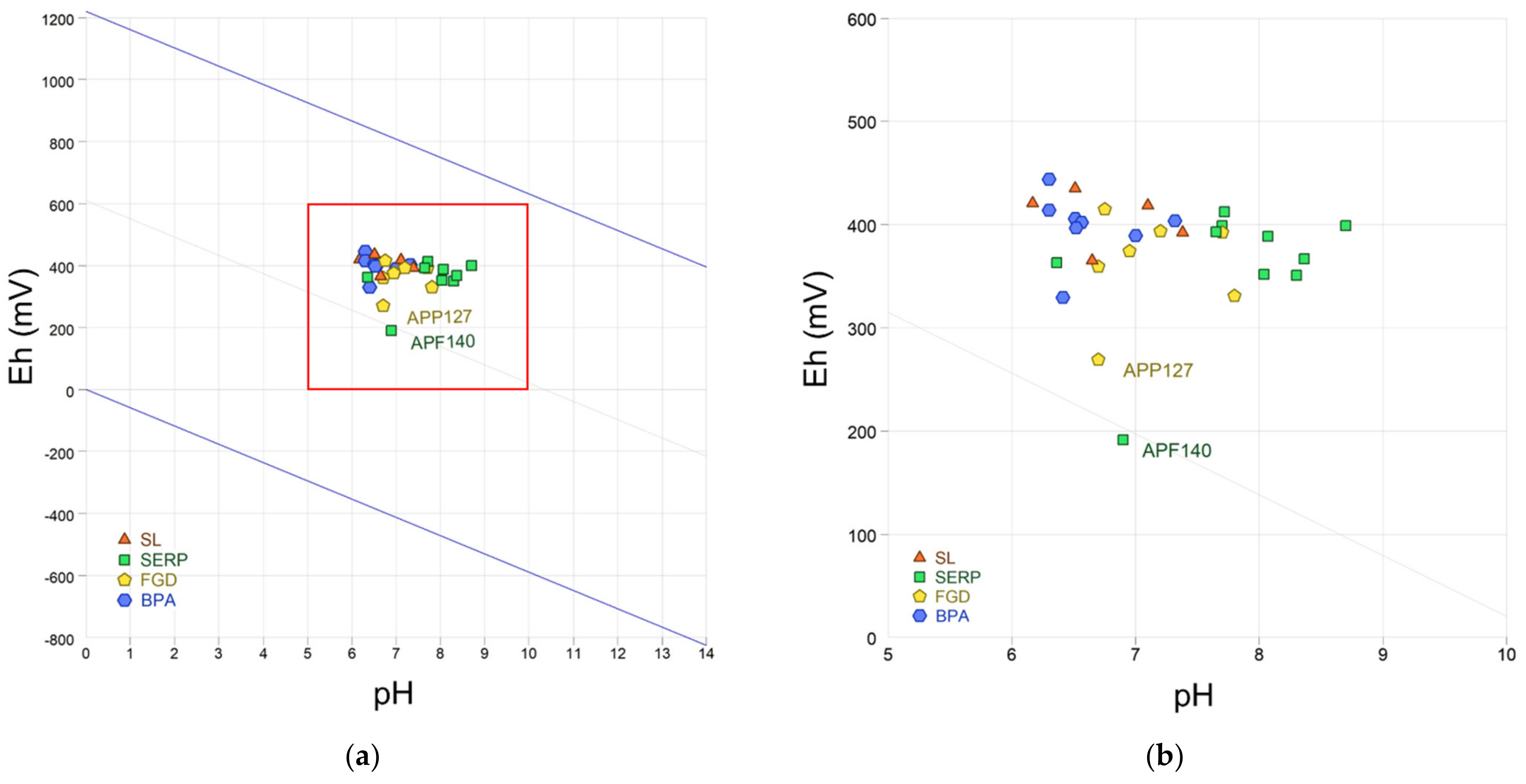
- APP127 (FGD), with a Mg-HCO3(SO4) facies. This MS is the only one where Co was detected, and has the second highest Fe concentration. These elements could be present in solution because of the relatively low redox potential. This station has been repeatedly monitored (Table S3), and the well stratigraphy has identified Mn oxide deposits;
- APF140 (SERP), an MS with low mineralisation and Mg-HCO3 facies. This MS shows the highest Fe concentration and is the only one with a reducing Eh (Figure 2);
- APE044 (BPA), with medium mineralisation and Mg-HCO3 facies. This MS has elevated Zn concentrations, but average Ni concentrations;
- APE059 (SERP), with medium–low mineralisation and Mg-HCO3 facies.
5.2.4. Iron
- APF140 (SERP) and APP127 (FGD), showing high Fe concentrations because of their low redox potential;
- APF082 (SL), with a low mineralisation and a Ca-HCO3 facies. The MS is located close to a rodingite vein, constituted by Ca-rich silicates hosting metallic ores [28];
- APF138 (SERP), with high mineralisation and Mg-SO4 facies. As previously discussed, this MS is located at the foothills of the Fandaglia mine waste dump and its Fe content could derive from oxidation of sulphides disseminated in serpentinite;
- APF092 (SL), with very low mineralisation and Mg(Ca)-HCO3 facies. This MS is very similar in hydrochemistry to APF082, and could contain Fe for the same reason.
5.2.5. Zinc
- APE044 (BPA), an MS already shown to have a high Mn concentration;
- APE041 (BPA), an MS with K+ concentrations higher than Na+, an uncommon feature in natural waters. Being located in the Balangero village, this well could reflect some anthropogenic contamination.
5.3. Statistical Distribution
5.4. Assessment of the Dataset
5.5. Evaluation of NBLs
6. Discussion
6.1. Comparison with Similar Hydrogeochemical Settings
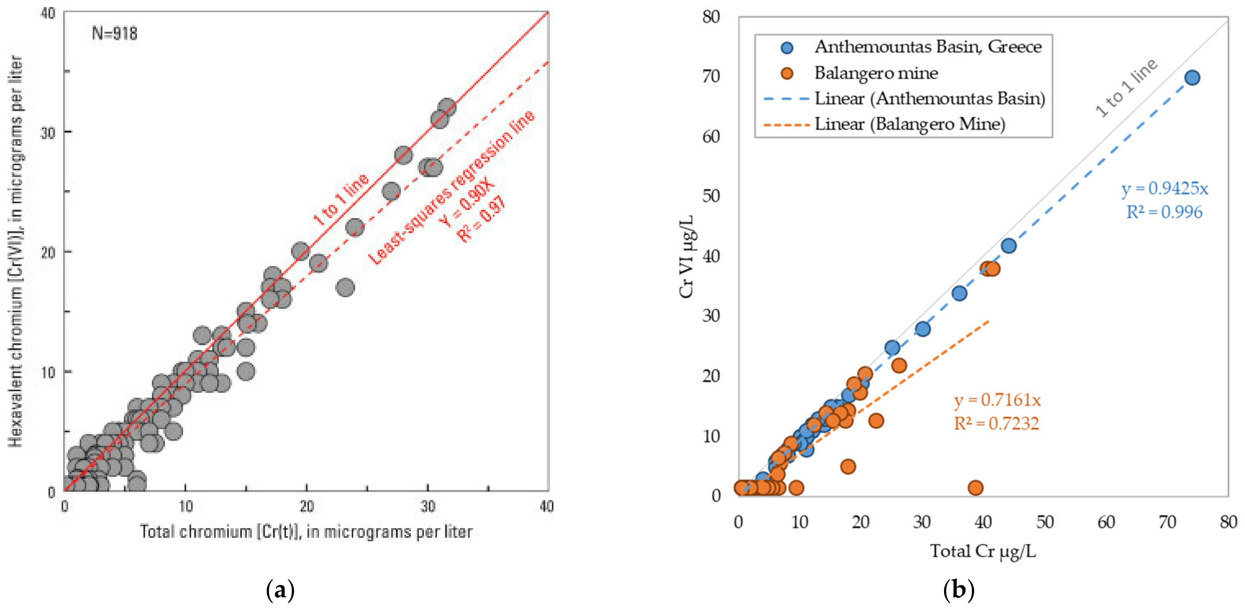
- the excellent linear correlation between Cr and Cr VI, with a slope close to one. Results of over 918 datapoints indicate that 90 ± 1% of Cr is in the Cr VI form, reaching concentrations very similar to those of our study site (Figure 4);
- the more frequent presence and the higher Cr VI concentrations found in alkaline waters (pH > 8) with respect to neutral or acidic waters. This is in agreement with the experimental results showing that Cr VI can be desorbed from mineral surfaces at a pH higher than 7.5;
- the more frequent presence and the higher Cr VI concentrations found in oxic waters (O2 > 0.5 mg/L) with respect to reducing waters;
- at comparable oxic conditions, the more frequent presence and the higher Cr VI concentrations found in deeper and older waters;
- the negative correlation of Cr VI with other PTEs, such as Fe2+, Mn2+ and Ni2+, which are soluble at low redox potential but less soluble in oxic conditions. The negative correlation between Cr VI and Ni is also found at our study site (N = 67; r = −0.33; p < 0.01).
6.2. Proposed NBLs
- APP127 (FGD) was monitored from 2015 for its elevated Mn contents (Table S3). It is located in an area where, for natural reasons, abundant Mn oxides are present. FGD is characterised by a low permeability that likely prevents the diffusion of atmospheric oxygen from the surface and permits the establishment of low redox conditions, favouring the solubilisation of Fe and Mn from the matrix;
- APF140 (SERP) was only sampled once and, according to the field notes, could not be adequately purged. The elevated Fe and Mn concentrations could therefore be related to the presence of stagnant water.
- the 95p values for Cr, Ni and Mn, where Ni and Mi will exceed the TVs for groundwater quality [22];
- the 90p values for Fe and Zn, which will not exceed the TVs.
7. Conclusions
Supplementary Materials
Author Contributions
Funding
Institutional Review Board Statement
Informed Consent Statement
Data Availability Statement
Acknowledgments
Conflicts of Interest
References
- Pourret, O.; Hursthouse, A. It’s time to replace the term “heavy metals” with “potentially toxic elements” when reporting environmental research. Int. J. Environ. Res. Public Health 2019, 16, 4446. [Google Scholar] [CrossRef] [PubMed] [Green Version]
- Bradl, H.; Kim, C.; Kramar, U.; StÜben, D. Heavy Metals in the Environment: Origin, Interaction and Remediation; Elsevier: Amsterdam, The Netherlands, 2005; ISBN 9780120883813. [Google Scholar]
- Meybeck, M. Heavy metal contamination in rivers across the globe: An indicator of complex interactions between societies and catchments. IAHS-AISH Proc. Rep. 2013, 361, 3–16. [Google Scholar]
- Zheng, S.; Zheng, X.; Chen, C. Leaching Behavior of Heavy Metals and Transformation of Their Speciation in Polluted Soil Receiving Simulated Acid Rain. PLoS ONE 2012, 7, 1–7. [Google Scholar] [CrossRef] [PubMed] [Green Version]
- World Health Organisation. Volume 1 Recommendations. In Guidelines for Drinking Water Quality, 2nd ed.; WHO: Geneva, Switzerland, 1993; ISBN 924154460. [Google Scholar]
- BRIDGE Background cRiteria for the IDentification of Groundwater Thresholds. Available online: http://nfp-at.eionet.europa.eu/irc/eionet-circle/bridge/info/data/en/index.htm (accessed on 1 March 2021).
- Vivona, R.; Preziosi, E.; Madé, B.; Giuliano, G. Occurrence of minor toxic elements in volcanic-sedimentary aquifers: A case study in central Italy. Hydrogeol. J. 2007, 15, 1183–1196. [Google Scholar] [CrossRef]
- Viaroli, S.; Cuoco, E.; Mazza, R.; Tedesco, D. Dynamics of natural contamination by aluminium and iron rich colloids in the volcanic aquifers of Central Italy. Environ. Sci. Pollut. Res. 2016, 23, 19958–19977. [Google Scholar] [CrossRef]
- Kazakis, N.; Kantiranis, N.; Voudouris, K.S.; Mitrakas, M.; Kaprara, E.; Pavlou, A. Geogenic Cr oxidation on the surface of mafic minerals and the hydrogeological conditions influencing hexavalent chromium concentrations in groundwater. Sci. Total Environ. 2015, 514, 224–238. [Google Scholar] [CrossRef]
- Rotiroti, M.; Bonomi, T.; Sacchi, E.; McArthur, J.M.; Jakobsen, R.; Sciarra, A.; Etiope, G.; Zanotti, C.; Nava, V.; Fumagalli, L.; et al. Overlapping redox zones control arsenic pollution in Pleistocene multi-layer aquifers, the Po Plain (Italy). Sci. Total Environ. 2021, 758, 143646. [Google Scholar] [CrossRef] [PubMed]
- Megremi, I.; Vasilatos, C.; Vassilakis, E.; Economou-Eliopoulos, M. Spatial diversity of Cr distribution in soil and groundwater sites in relation with land use management in a Mediterranean region: The case of C. Evia and Assopos-Thiva Basins, Greece. Sci. Total Environ. 2019, 651, 656–667. [Google Scholar] [CrossRef] [PubMed]
- Barceloux, D.G.; Barceloux, D. Chromium. J. Toxicol. Clin. Toxicol. 1999, 37, 173–194. [Google Scholar] [CrossRef]
- GWD Directive 2006/118/EC of the European Parliament and of the Council of 12 December 2006 on the protection of groundwater against pollution and deterioration. Off. J. Eur. Union 2006, L372, 19–31.
- WFD Directive 2000/60/EC of the European Parliament and of the Council of 23 October 2000 establishing a framework for Community action in the field of water policy. Off. J. Eur. Union 2000, L327, 1–73.
- D. Lgs n. 152/2006. Norme in materia ambientale. Gazz. Uff. Ser. Gen. 2006, 88, 592. Available online: https://www.minambiente.it/sites/default/files/dlgs_03_04_2006_152.pdf (accessed on 1 March 2021).
- Rotiroti, M.; Di Mauro, B.; Fumagalli, L.; Bonomi, T. COMPSEC, a new tool to derive natural background levels by the component separation approach: Application in two different hydrogeological contexts in northern Italy. J. Geochemical Explor. 2015, 158, 44–54. [Google Scholar] [CrossRef]
- Preziosi, E.; Giuliano, G.; Vivona, R. Natural background levels and threshold values derivation for naturally As, V and F rich groundwater bodies: A methodological case study in Central Italy. Environ. Earth Sci. 2010, 61, 885–897. [Google Scholar] [CrossRef]
- De Caro, M.; Crosta, G.B.; Frattini, P. Hydrogeochemical characterization and Natural Background Levels in urbanized areas: Milan Metropolitan area (Northern Italy). J. Hydrol. 2017, 547, 455–473. [Google Scholar] [CrossRef]
- Güler, C.; Thyne, G.D.; Tala, H.; Yjldjrjm, Ü. Processes governing alkaline groundwater chemistry within a fractured rock (Ophiolitic mélange) aquifer underlying a seasonally inhabited headwater area in the aladallar range (Adana, Turkey). Geofluids 2017, 2017, 13–15. [Google Scholar] [CrossRef]
- Heikkinen, P.M.; Korkka-Niemi, K.; Lahti, M.; Salonen, V.P. Groundwater and surface water contamination in the area of the Hitura nickel mine, Western Finland. Environ. Geol. 2002, 42, 313–329. [Google Scholar]
- Blowes, D.W.; Ptacek, C.J.; Jambor, J.L.; Weisener, C.G. The Geochemistry of Acid Mine Drainage. In Treatise on Geochemistry; Holland, H.H., Turekian, K.K., Eds.; Elsevier: Amsterdam, The Netherlands, 2003; pp. 149–204. ISBN 9780080437514. [Google Scholar]
- ISPRA. Linee guida per la determinazione dei valori di fondo per i suoli e le acque sotterranee, Delibera del Consiglio SNPA. In Seduta del 14.11.2017. Doc. n. 20/2017; ISPRA: Rome, Italy, Manuali e Linee Guida 174/2018; 2018; ISBN 978-88-448-0880-8. Available online: https://www.isprambiente.gov.it/files2018/pubblicazioni/manuali-linee-guida/MLG_174_18.pdf (accessed on 1 March 2021).
- Piccardo, G.B. The Lanzo peridotite massif, Italian Western Alps: Jurassic rifting of the Ligurian Tethys. Geol. Soc. London Spec. Publ. 2010, 337, 47–69. [Google Scholar] [CrossRef]
- Piccardo, G.B.; Padovano, M.; Guarnieri, L. The Ligurian Tethys: Mantle processes and geodynamics. Earth Sci. Rev. 2014, 138, 409–434. [Google Scholar] [CrossRef]
- Ferraris, C.; Compagnoni, R. Metamorphic evolution and significance of a serpentinized peridotite slice within the Eclogitic Micaschist Complex of the Sesia-Zone (Western Alps, Italy). Schweizerische Mineralogische und Petrographische Mitteilungen 2003, 83, 3–13. [Google Scholar]
- Comune di Balangero Piano Regolatore Comunale Generale. Available online: http://www.comune.balangero.to.it/Home/Menu?IDDettaglio=135816 (accessed on 19 February 2021).
- Rossetti, P.; Zucchetti, S. Early-alpine ore parageneses in the serpentinites from the Balangero asbestos mine and Lanzo Massif (Internal Western Alps). Rend. Della Soc. Ital. Mineral. Petrol. 1988, 43, 139–149. [Google Scholar]
- Rossetti, P.; Zucchetti, S. Occurrence of native iron, Fe-Co and Ni-Fe alloys in the serpentinite from the Balangero asbestos mine (Western Italian Alps). Ofioliti 1988, 13, 43–56. [Google Scholar]
- Castelli, D.; Rossetti, P. Sulphide-arsenide mineralization in rodingite from the Balangero mine (Italian Western Alps): Hydrothermalism related to metamorphic fluids. In Proceedings of the Giornata di Studio in Ricordo Del Prof. Stefano Zucchetti, Turin, Italy, 12 May 1994; pp. 103–110. [Google Scholar]
- Castelli, D.; Rolfo, F.; Rossetti, P. Petrology of ore-bearing rodingite veins from the Balangero asbestos mine (Western Alps). Boll. Mus. Regionale Sci. Nat. Torino 1995, 13, 153–189. [Google Scholar]
- Groppo, C.; Compagnoni, R. Metamorphic veins from the serpentinites of the Piemonte Zone, western Alps, Italy: A review. Period. Mineral. 2007, 76, 127–153. [Google Scholar]
- Zucchetti, S.; Mastrangelo, F.; Rossetti, P.; Sandrone, R. Serpentinization and metamorphism: Their relationships with metallogeny in some ophiolitic ultramafics from the Alps. In Proceedings of the Zuffar’ Days Symposium, Cagliari, Italy, 10–15 October 1988; pp. 137–159. [Google Scholar]
- Ferrante, D.; Mirabelli, D.; Silvestri, S.; Azzolina, D.; Giovannini, A.; Tribaudino, P.; Magnani, C. Mortality and mesothelioma incidence among chrysotile asbestos miners in Balangero, Italy: A cohort study. Am. J. Ind. Med. 2020, 63, 135–145. [Google Scholar] [CrossRef] [PubMed]
- Paglietti, F.; Gennari, F.; Giangrasso, M. The asbestos extraction in the Balangero mine: Environmental consequences. In Proceedings of the Goldschmidt Conference Abstracts, Davos, Switzerland, 21–26 June 2009; p. A985. Available online: https://goldschmidtabstracts.info/abstracts/abstractView?id=2009001620 (accessed on 1 March 2021).
- Parrone, D.; Frollini, E.; Preziosi, E.; Ghergo, S. eNaBLe, an On-Line Tool to Evaluate Natural Background Levels in Groundwater Bodies. Water 2020, 13, 74. [Google Scholar] [CrossRef]
- APAT; CNR-IRSA. Metodi Analitici per le Acque; Manuali e Linee Guida 29/2003; APAT: Rome, Italy, 2003; ISBN 88-448-0083-7. [Google Scholar]
- Pourbaix, M. Atlas of Electrochemical Equilibria in Aqueous Solution, 1st ed.; Pergamon Press: Bristol, UK, 1966. [Google Scholar]
- Edmunds, W.M.; Shand, P. (Eds.) Natural Groundwater Quality; Blackwell Publishing: Hoboken, NJ, USA, 2008; ISBN 978-14051-5675-2. [Google Scholar]
- Piper, A.M. A graphic procedure in geochemical interpretation of water analyses. Trans. Am. Geophys. Union 1944, 25, 914–923. [Google Scholar] [CrossRef]
- Stiff, H.A.J. The interpretation of chemical water analysis by means of patterns. J. Pet. Technol. 1951, 3, 15–16. [Google Scholar] [CrossRef]
- Vitale Brovarone, A.; Martinez, I.; Elmaleh, A.; Compagnoni, R.; Chaduteau, C.; Ferraris, C.; Esteve, I. Massive production of abiotic methane during subduction evidenced in metamorphosed ophicarbonates from the Italian Alps. Nat. Commun. 2017, 8, 14134. [Google Scholar] [CrossRef] [PubMed]
- Mann, H. Nonparametric tests against trend. Econometrica 1945, 13, 245–259. [Google Scholar] [CrossRef]
- Kendall, M.G. Rank Correlation Methods, 3rd ed.; Hafner: New York, NY, USA, 1962. [Google Scholar]
- Meals, D.W.; Spooner, J.; Dressing, S.A.; Harcum, J.B. Statistical Analysis for Monotonic Trends; Tetra Tech, Inc.: Fairfax, VA, USA, 2011. Available online: https://www.epa.gov/sites/production/files/2016-05/documents/tech_notes_6_dec2013_trend.pdf (accessed on 1 March 2021).
- Sen, P.K. Estimates of the regression coefficient based on Kendall’s tau. J. Am. Stat. Assoc. 1968, 63, 1379–1389. [Google Scholar] [CrossRef]
- Shapiro, S.S.; Wilk, M.B. An analysis of variance test for normality (complete samples). Biometrika 1965, 52, 591–611. [Google Scholar] [CrossRef]
- D’Agostino, R.B.; Belanger, A.; D’Agostino, R.B. A Suggestion for Using Powerful and Informative Tests of Normality. Am. Stat. 1990, 44, 316–321. [Google Scholar]
- De Vos, W.; Tarvainen, T.; Salminen, R.; Reeder, S.; De Vivo, B.; Demetriades, A.; Pirc, S.; Batista, M.J.; Marsina, K.; Ottesen, R.-T.; et al. Geochemical Atlas of Europe. Part 2—Interpretation of Geochemical Maps, Additional Tables, Figures, Maps, and Related Publications; De Vos, W., Tarvainen, T., Eds.; Geological Survey of Finland, Espoo: Espoo, Finland, 2006; ISBN 951-690-956-6. [Google Scholar]
- ARPA Piemonte. Definizione dei Valori di Fondo Naturale per i Metalli Nelle Acque Sotterranee Come Previsto Dalla Direttiva 2006/118/CE e dal Decreto Legislativo 16 Marzo 2009 n.30; ARPA Piemonte: Turin, Italy, 2012; Available online: https://www.arpa.piemonte.it/approfondimenti/temi-ambientali/acqua/acque-sotterranee/Relazionevaloridifondosotterranee.pdf (accessed on 1 March 2021).
- Langone, A.; Baneschi, I.; Boschi, C.; Dini, A.; Guidi, M.; Cavallo, A. Serpentinite-water interaction and chromium(VI) release in spring waters: Examples from Tuscan ophiolites. Ofioliti 2013, 38, 41–57. [Google Scholar]
- Apollaro, C.; Fuoco, I.; Brozzo, G.; De Rosa, R. Release and fate of Cr(VI) in the ophiolitic aquifers of Italy: The role of Fe(III) as a potential oxidant of Cr(III) supported by reaction path modelling. Sci. Total Environ. 2019, 660, 1459–1471. [Google Scholar] [CrossRef]
- McClain, C.N.; Fendorf, S.; Webb, S.M.; Maher, K. Quantifying Cr(VI) Production and Export from Serpentine Soil of the California Coast Range. Environ. Sci. Technol. 2017, 51, 141–149. [Google Scholar] [CrossRef] [PubMed]
- Izbicki, J.A.; Wright, M.T.; Seymour, W.A.; McCleskey, R.B.; Fram, M.S.; Belitz, K.; Esser, B.K. Cr(VI) occurrence and geochemistry in water from public-supply wells in California. Appl. Geochem. 2015, 63, 203–217. [Google Scholar] [CrossRef] [Green Version]
- Iribar, V. Origin of neutral mine water in flooded underground mines: An appraisal using geochemical and hydrogeological methodologies. In Proceedings of the Mine Water 2004-Proceedings International Mine Water Association Symposium, Newcastle upon Tyne, UK, 20–25 September 2004; Volume 1, pp. 169–178. Available online: https://www.imwa.info/docs/imwa_2004/IMWA2004_22_Iribar.pdf (accessed on 1 March 2021).
- Frau, F.; Medas, D.; Da Pelo, S.; Wanty, R.B.; Cidu, R. Environmental effects on the aquatic system and metal discharge to the mediterranean sea from a near-neutral zinc-ferrous sulfate mine drainage. Water. Air. Soil Pollut. 2015, 226, 1–17. [Google Scholar] [CrossRef]


| Monitoring Station | Unit | Cr µg/L | Cr VI µg/L | Co µg/L | Ni µg/L | Mn µg/L | Fe µg/L | Zn µg/L |
|---|---|---|---|---|---|---|---|---|
| APE031 | BPA | 1.0 | 1.5 | 0.5 | 71.3 | 1.3 | 7.2 | 38.4 |
| APS096 | FGD | 4.8 | 1.5 | 0.5 | 23.9 | 5.8 | 1.6 | 0.5 |
| APP126 | FGD | 17.8 | 14.1 | 0.5 | 1.7 | 0.5 | 0.5 | 0.5 |
| APF082 | SL | 11.0 | 3.3 | 0.5 | 20.4 | 4.4 | 329.9 | 15.5 |
| APP128 | SL | 4.7 | 3.6 | 0.5 | 14.4 | 8.1 | 0.5 | 0.5 |
| APP127 | FGD | 0.5 | 1.5 | 2.9 | 8.9 | 1571.5 | 966.0 | 0.5 |
| APE059 | SERP | 4.5 | 1.5 | 0.5 | 26.6 | 17.7 | 3.4 | 0.5 |
| ASS078 | SERP | 6.7 | 1.5 | 0.5 | 8.7 | 2.3 | 4.3 | 0.5 |
| ASS058 | SERP | 1.4 | 1.5 | 0.5 | 2.5 | 0.5 | 8.6 | 0.5 |
| ASS080 | SERP | 2.7 | 1.5 | 0.5 | 8.5 | 1.0 | 3.5 | 0.5 |
| APE047 | BPA | 1.6 | 1.5 | 0.5 | 56.6 | 0.5 | 0.5 | 0.5 |
| APE108 | BPA | 2.4 | 1.5 | 0.5 | 32.3 | 2.5 | 0.5 | 46.2 |
| APE044 | BPA | 0.5 | 1.5 | 0.5 | 37.8 | 22.0 | 7.9 | 213.5 |
| APE045 | BPA | 0.5 | 1.5 | 0.5 | 37.5 | 2.7 | 0.5 | 33.7 |
| APE041 | BPA | 3.9 | 1.5 | 0.5 | 6.1 | 0.5 | 0.5 | 57.0 |
| APE046 | BPA | 5.4 | 1.5 | 0.5 | 2.5 | 0.5 | 0.5 | 27.0 |
| APP091 | FGD | 1.7 | 1.5 | 0.5 | 5.6 | 0.5 | 1.1 | 21.4 |
| APE110 | FGD | 3.6 | 1.5 | 0.5 | 17.7 | 0.5 | 0.5 | 11.4 |
| APF092 | SL | 0.5 | 1.5 | 0.5 | 1.4 | 6.8 | 30.0 | 0.9 |
| ASP013 | SERP | 8.5 | 3.8 | 0.5 | 34.1 | 0.5 | 0.5 | 0.5 |
| APP083 | FGD | 6.8 | 6.7 | 0.5 | 0.9 | 0.5 | 3.4 | 0.5 |
| ASS79 | SL | 4.8 | 1.5 | 0.5 | 16.0 | 4.0 | 0.5 | 0.5 |
| APF111 | SERP | 3.9 | 1.5 | 0.5 | 12.1 | 0.5 | 0.5 | 0.5 |
| APF139 | SERP | 0.5 | 1.5 | 0.5 | 8.9 | 2.1 | 19.5 | 0.5 |
| APF005 | SERP | 41.0 | 38.1 | 0.5 | 0.5 | 0.5 | 1.5 | 0.5 |
| APF138 | SERP | 1.9 | 1.5 | 0.5 | 1.6 | 6.8 | 38.9 | 0.5 |
| APF140 | SERP | 0.5 | 1.5 | 0.5 | 0.5 | 125.0 | 1583.0 | 0.5 |
| ASM137 | FGD | 0.5 | 1.5 | 0.5 | 15.8 | 0.5 | 0.5 | 0.5 |
| ASC077 | SL | 0.5 | 1.5 | 0.5 | 0.5 | 5.3 | 0.5 | 3.6 |
| MS | 29 | 29 | 29 | 29 | 29 | 29 | 29 | |
| < LOD | 8 | 23 | 28 | 3 | 12 | 12 | 18 | |
| % ND | 28 | 79 | 97 | 10 | 41 | 41 | 62 |
| Including ND Data | Cr | Cr VI | Co | Ni | Mn | Fe | Zn | |
|---|---|---|---|---|---|---|---|---|
| N | Valid | 29 | 29 | 29 | 29 | 29 | 29 | 29 |
| Missing | 0 | 0 | 0 | 0 | 0 | 0 | 0 | |
| Mean | 4.965 | 3.588 | 0.583 | 16.376 | 61.898 | 104.007 | 16.466 | |
| Median | 2.700 | 1.500 | 0.500 | 8.900 | 2.100 | 1.500 | 0.500 | |
| Mode | 0.5 | 1.5 | 0.5 | 0.5 | 0.5 | 0.5 | 0.5 | |
| Std. Deviation | 7.9155 | 7.0997 | 0.4457 | 17.7297 | 291.25 | 340.02 | 41.0952 | |
| Skewness | 3.730 | 4.511 | 5.385 | 1.554 | 5.333 | 3.768 | 4.245 | |
| Kurtosis | 16.028 | 21.586 | 29.000 | 2.382 | 28.596 | 14.339 | 20.118 | |
| Minimum | 0.5 | 1.5 | 0.5 | 0.5 | 0.5 | 0.5 | 0.5 | |
| Maximum | 41.0 | 38.1 | 2.9 | 71.3 | 1571.5 | 1583.0 | 213.5 | |
| Percentiles | 25 | 0.500 | 1.500 | 0.500 | 2.100 | 0.500 | 0.500 | 0.500 |
| 50 | 2.700 | 1.500 | 0.500 | 8.900 | 2.100 | 1.500 | 0.500 | |
| 75 | 5.100 | 1.500 | 0.500 | 25.250 | 6.300 | 8.225 | 18.425 | |
| 90 | 11.000 | 6.650 | 0.500 | 37.800 | 21.950 | 329.90 | 46.200 | |
| 95 | 29.400 | 26.100 | 1.700 | 63.925 | 848.25 | 1274.0 | 135.25 | |
| Excluding ND | Cr | Cr VI | Co | Ni | Mn | Fe | Zn | |
|---|---|---|---|---|---|---|---|---|
| N | Valid | 21 | 6 | 1 | 26 | 17 | 16 | 11 |
| Missing | 8 | 23 | 28 | 3 | 12 | 13 | 18 | |
| Mean | 6666 | 11.592 | 2.900 | 18.208 | 105.238 | 188.106 | 42.591 | |
| Median | 4500 | 5.225 | 2.900 | 13.225 | 5.300 | 7.525 | 27.000 | |
| Mode | 3.9 a | 3.3 a | 2.9 | 2.5 | 6.8 | 1.1 a | 0.8 a | |
| Std. Deviation | 8.7581 | 13.6142 | 17.8417 | 378.98 | 446.08 | 59.3218 | ||
| Skewness | 3.373 | 2.017 | 1.480 | 4.083 | 2.672 | 2.810 | ||
| Kurtosis | 12.675 | 4.079 | 2.138 | 16.755 | 6.774 | 8.570 | ||
| Minimum | 1.0 | 3.3 | 2.9 | 0.8 | 1.0 | 1.1 | 0.8 | |
| Maximum | 41.0 | 38.1 | 2.9 | 71.3 | 1571.5 | 1583.0 | 213.5 | |
| Percentiles | 25 | 2.150 | 3.525 | 2.900 | 4.788 | 2.350 | 3.362 | 11.400 |
| 50 | 4.500 | 5.225 | 2.900 | 13.225 | 5.300 | 7.525 | 27.000 | |
| 75 | 6.725 | 20.100 | 2.900 | 28.013 | 12.875 | 36.675 | 46.200 | |
| 90 | 16.440 | 38.100 | 2.900 | 43.425 | 414.30 | 1151.1 | 182.20 | |
| 95 | 38.680 | 38.100 | 2.900 | 66.137 | 1571.5 | 1583.0 | 213.50 | |
| Including ND | Cr | Cr VI | Co | Ni | Mn | Fe | Zn | |
|---|---|---|---|---|---|---|---|---|
| N | Valid | 71 | 67 | 71 | 71 | 74 | 39 | 39 |
| Missing | 3 | 7 | 3 | 3 | 0 | 35 | 35 | |
| Mean | 4.965 | 6.979 | 5.473 | 0.654 | 21.332 | 183.1 | 87.249 | |
| Median | 2.700 | 3.1 | 1.5 | 0.5 | 9.1 | 1.1 | 1.7 | |
| Mode | 0.5 | 0.5 | 1.5 | 0.5 | 0.5 | 0.5 | 0.5 | |
| Std. Deviation | 7.9155 | 9.51 | 7.909 | 0.915 | 25.790 | 844.760 | 305.937 | |
| Skewness | 3.730 | 2.139 | 2.591 | 5.959 | 1.519 | 5.401 | 4.042 | |
| Kurtosis | 16.028 | 4.584 | 7.392 | 35.02 | 1.764 | 30.038 | 16.787 | |
| Minimum | 0.5 | 0.5 | 1.5 | 0.5 | 0.5 | 0.5 | 0.5 | |
| Maximum | 41.0 | 41.4 | 38.1 | 6.6 | 109 | 5554 | 1583 | |
| Percentiles | 25 | 0.5 | 1.5 | 0.5 | 1.8 | 0.5 | 0.5 | 0.5 |
| 50 | 3.1 | 1.5 | 0.5 | 9.1 | 1.1 | 1.7 | 0.5 | |
| 75 | 7.4 | 6.5 | 0.5 | 34 | 6.05 | 8 | 11.4 | |
| 90 | 19.6 | 15.0 | 0.5 | 64.06 | 46.74 | 58.40 | 57.00 | |
| 95 | 31.1 | 21.4 | 0.5 | 78.78 | 1568.75 | 966 | 120 | |
| Excluding ND | Cr | Cr VI | Co | Ni | Mn | Fe | Zn | |
|---|---|---|---|---|---|---|---|---|
| N | Valid | 53 | 21 | 2 | 63 | 38 | 21 | 13 |
| Missing | 21 | 53 | 72 | 11 | 36 | 53 | 61 | |
| Mean | 6666 | 9.179 | 14.176 | 5.95 | 23.978 | 356.089 | 161.605 | |
| Median | 4500 | 5.4 | 12.8 | 5.95 | 12.1 | 5.55 | 6.4 | |
| Mode | 3.9 a | 1.6 | 12.8 a | 5.3 a | 1.2a | 1.8 | 1.6 a | |
| Std. Deviation | 8.7581 | 10.1134 | 9.5163 | 0.9192 | 26.2264 | 1159.6447 | 406.5181 | |
| Skewness | 3.373 | 1.824 | 1.526 | 1.39 | 3.759 | 2.829 | ||
| Kurtosis | 12.675 | 3.085 | 2.253 | 1.355 | 14.046 | 7.774 | ||
| Minimum | 1.0 | 1 | 3.8 | 5.3 | 1.1 | 1 | 1.6 | |
| Maximum | 41.0 | 41.4 | 38.1 | 6.6 | 109 | 5554 | 1583 | |
| Percentiles | 25 | 1.85 | 6.65 | 5.3 | 3.4 | 2.475 | 2.65 | 7.5 |
| 50 | 5.4 | 12.8 | 5.95 | 12.1 | 5.55 | 6.4 | 33.7 | |
| 75 | 14.75 | 18.1 | 6.6 | 34.3 | 21.1 | 29.85 | 66.65 | |
| 90 | 21.68 | 34.88 | 6.6 | 68.86 | 1567.1 | 900.6 | 232.2 | |
| 95 | 39.2 | 38.1 | 6.6 | 82.26 | 4392.15 | 1521.3 | 307 | |
| Data from Table 1 Without ND | Excluding the MSs APP127 and APF140 | |||||||
|---|---|---|---|---|---|---|---|---|
| N | Max | 95p | 90p | N | Max | 95p | 90p | |
| Cr | 21 | 41 | 38.7 | 16.44 | 21 | 41 | 38.7 | 16.44 |
| Cr VI | 6 | 38.1 | 38.1 | 38.1 | 6 | 38.1 | 38.1 | 38.1 |
| Co | 1 | 2.9 | 2.9 | 2.9 | 0 | NA | NA | NA |
| Ni | 26 | 71.3 | 66.1 | 43.42 | 25 | 71.3 | 66.9 | 45.3 |
| Mn | 17 | 1571.5 | 1571.5 | 414.3 | 15 | 22.0 | 21.95 | 19.4 |
| Fe | 16 | 1583 | 1583 | 1151.1 | 14 | 329.9 | 329.9 | 184.4 |
| Zn | 11 | 213.5 | 213.5 | 182.2 | 11 | 213.5 | 213.5 | 182.2 |
| Data from Table S3 Without ND | Excluding Data from APP127 and APF140 | |||||||
|---|---|---|---|---|---|---|---|---|
| N | Max | 95p | 90p | N | Max | 95p | 90p | |
| Cr | 52 | 41.4 | 39.2 | 21.68 | 52 | 41.4 | 39.3 | 21.86 |
| Cr VI | 21 | 38.1 | 38.1 | 34.88 | 21 | 38.1 | 38.1 | 34.88 |
| Co | 2 | 6.6 | 6.6 | 6.6 | 0 | NA | NA | NA |
| Ni | 63 | 109 | 82.26 | 68.86 | 59 | 109 | 84.0 | 71.3 |
| Mn | 38 | 5554 | 4392 | 1567 | 32 | 92.1 | 71.36 | 27.22 |
| Fe | 21 | 1583 | 1521 | 900.6 | 19 | 639 | 630 | 58.4 |
| Zn | 13 | 307 | 307 | 232.2 | 13 | 307 | 307 | 232.2 |
| Cr | Cr VI | Fe | Mn | Ni | ||
|---|---|---|---|---|---|---|
| N | Valid | 541 | 96 | 494 | 474 | 445 |
| Missing | 18 | 463 | 65 | 85 | 114 | |
| Mean | 7.58 | 15.26 | 25.78 | 2.93 | 13.73 | |
| Median | 4.00 | 12.00 | 8.00 | 0.00 | 5.40 | |
| Mode | 2.00 | 3.00 | 0.00 | 0.00 | 0.00 | |
| Std. Deviation | 9.71 | 14.64 | 72.36 | 27.80 | 23.01 | |
| Skewness | 2921.23 | 1718.94 | 8321.03 | 19147.22 | 4701.43 | |
| Kurtosis | 11297.90 | 4002.48 | 91757.03 | 392675.03 | 35534.60 | |
| Minimum | 0.02 | 0.05 | 0.00 | 0.00 | 0.00 | |
| Maximum | 73.00 | 73.00 | 948.00 | 579.00 | 259.60 | |
| Percentiles | 25 | 2.00 | 3.00 | 0.000 | 0.00 | 1.15 |
| 50 | 4.00 | 12.00 | 8.00 | 0.00 | 5.40 | |
| 75 | 9.00 | 21.00 | 19.00 | 0.77 | 18.00 | |
| 95 | 28.90 | 42.75 | 127.00 | 5.98 | 52.77 | |
| 99 | 46.17 | 73.00 | 304.05 | 51.10 | 121.16 | |
| Percentile | Proposed NBL in μg/L | |
|---|---|---|
| Cr | 95p | 39.3 |
| Cr VI | 95p | 38.1 * |
| Co | - | ND |
| Ni | 95p | 84 |
| Mn | 95p | 71.36 |
| Fe | 90p | 58.4 |
| Zn | 90p | 232.2 |
Publisher’s Note: MDPI stays neutral with regard to jurisdictional claims in published maps and institutional affiliations. |
© 2021 by the authors. Licensee MDPI, Basel, Switzerland. This article is an open access article distributed under the terms and conditions of the Creative Commons Attribution (CC BY) license (http://creativecommons.org/licenses/by/4.0/).
Share and Cite
Sacchi, E.; Bergamini, M.; Lazzari, E.; Musacchio, A.; Mor, J.-R.; Pugliaro, E. Natural Background Levels of Potentially Toxic Elements in Groundwater from a Former Asbestos Mine in Serpentinite (Balangero, North Italy). Water 2021, 13, 735. https://doi.org/10.3390/w13050735
Sacchi E, Bergamini M, Lazzari E, Musacchio A, Mor J-R, Pugliaro E. Natural Background Levels of Potentially Toxic Elements in Groundwater from a Former Asbestos Mine in Serpentinite (Balangero, North Italy). Water. 2021; 13(5):735. https://doi.org/10.3390/w13050735
Chicago/Turabian StyleSacchi, Elisa, Massimo Bergamini, Elisa Lazzari, Arianna Musacchio, Jordi-René Mor, and Elisa Pugliaro. 2021. "Natural Background Levels of Potentially Toxic Elements in Groundwater from a Former Asbestos Mine in Serpentinite (Balangero, North Italy)" Water 13, no. 5: 735. https://doi.org/10.3390/w13050735