CFD Modelling of the Transport of Soluble Pollutants from Sewer Networks to Surface Flows during Urban Flood Events

Abstract

Surcharging urban drainage systems are a potential source of pathogenic contamination of floodwater. While a number of previous studies have investigated net sewer to surface hydraulic flow rates through manholes and gullies during flood events, an understanding of how pollutants move from sewer networks to surface flood water is currently lacking. This paper presents a 3D CFD model to quantify flow and solute mass exchange through hydraulic structures featuring complex interacting pipe and surface flows commonly associated with urban flood events. The model is compared against experimental datasets from a large-scale physical model designed to study pipe/surface interactions during flood simulations. Results show that the CFD model accurately describes pipe to surface flow partition and solute transport processes through the manhole in the experimental setup. After validation, the model is used to elucidate key timescales which describe mass flow rates entering surface flows from pipe networks. Numerical experiments show that following arrival of a well-mixed solute at the exchange structure, solute mass exchange to the surface grows asymptotically to a value equivalent to the ratio of flow partition, with associated timescales a function of the flow conditions and diffusive transport inside the manhole.

1. Introduction

Urban flooding events can cause significant economic and societal disruption. Numerous studies [1,2,3] have suggested that the occurrence of flooding in urban areas is likely to increase in the future due to increased urbanisation and changes in precipitation patterns, making intense rainfall events and the inundation of local drainage systems more common. The majority of urban flooding hazard studies focus on the economic damage, or direct risks to the public derived from hydraulic modelling of the depth and velocity of floodwaters resulting from historic or design rainfall events (see, e.g., in [4,5]). However, an increasing number of studies have also considered the public health risks of exposure to flood water, which may take the form of long term mental impacts [6], or illness from direct exposure of the public to contaminated flood water. Urban floodwater may contain a mix of rainwater, stormwater runoff and waste/foul water from surcharging urban drainage systems and therefore may contain harmful bacteria [7,8]. For example, ten Veldhuis et al. [9] sampled and analysed flood water from three urban flooding incidents in the Hague, the Netherlands in areas served by combined sewers. In the study, values of intestinal enterococci and E. coli were found to be 1 to 3 orders of magnitude higher than values for good bathing water quality according to the EU Directive 2006/7/EC.

Understanding the concentrations, transport and fate of harmful contaminants in urban floodwaters for effective health risk assessment is challenging [10]. Current state of the art urban flood risk models consider urban hydrological processes and utilise hydrodynamic principles to route resulting flows in both piped drainage and surface overland systems, with interaction (i.e., mass transfer) nodes such as manholes or gullies, which are commonly represented by weir or orifice equations [11,12,13]. Although flood model calibration and validation is often difficult due to a paucity of full scale data, such tools are generally considered to give tolerable predictions of flood depths and are widely used for risk evaluation and asset management [14]. Recently, Mark et al. [15] developed an approach to integrate an understanding of contaminant transport and health risk into flood models, utilising the 2D Advection Dispersion Equation to simulate the mixing and transport of wastewater surcharging from drainage systems within overland surface flow (assuming a constant pathogen level within the surcharging flow). However, such approaches can significantly simplify a number of processes concerning sources, transport, survival and transformations of harmful contaminants (e.g., see in [10]). The number of additional terms and associated parameters required to account for transport and fate processes exacerbate non-identifiability and equifinality issues which are a common problem for complex integrated models [16]. To develop a more robust understanding of health risks posed by urban flood waters, detailed information is required concerning individual processes associated with sources, transport pathways and life cycles of pathogens from sewer/drainage networks to surface flows and on urban surfaces. For example, recent studies have considered the behaviour of waterborne pathogens on different urban surfaces [17] and evaluation of pathogen levels in urban rainfall runoff flows [18].

However, as far as the authors are aware, no studies to date have considered the exchange of contaminated material (in soluble or particulate form) from drainage/sewer networks to surface flows during flood events via interaction structures such as gullies and/or manholes. Flows in and around surcharging hydraulic structures are highly complex and three-dimensional, especially during interactions with surface flood flows [19]. It is also likely that contamination concentrations within urban drainage/sewer networks will vary significantly as the proportion of stormwater and quantity and nature of contaminated material (i.e., dissolved vs. entrained solids) within the network varies during flood events. Numerous studies have considered the mixing of soluble material in manhole structures in the absence of interacting surface flood flows, demonstrating that mixing/transport (and thus mass exchange) processes are sensitive to geometrical characteristics and poorly described using commonly used simple models such as the 1D ADE which are commonly used to model pollutant transport and mixing in piped networks (see, e.g., in [20,21]). More complex 3D CFD based approaches have been shown to be able to quantify hydraulic and solute mixing processes in hydraulic structures such as manholes [12,22,23,24,25]. However, to date such models have not been experimentally validated in urban flood situations which include complex interactions between piped and surface flows [19]. While such 3D models are too computationally expensive to be used in direct design or network simulation, validated CFD models can be used to conduct experiments which may elucidate relationships and timescales describing the transport of materials to surface flows, understand the influence of geometric or hydraulic variables on mixing and mass transport characteristics or be used to calibrate simpler models.

Understanding how contaminants move from sewer networks to surface flows is a key aspect for understanding health risks posed by urban floods and possibly to foster the design of techniques to mitigate negative effects. This study conducts a detailed 3D numerical simulation of flow and soluble mass transport through a manhole during surface flooding conditions where net sewer to surface exchange flows are simulated. Whilst the focus of this study is limited to soluble pollutants only (i.e., those fully dissolved in the flow), it is recognised that the transport of contaminated solid material (e.g., fine sewer sediments) is also relevant in this context. The aims of the paper are to (1) compare the model outputs to new hydraulic and solute transport experimental datasets collected in a scale model facility designed to study interactions between pipe and surface flows. (2) Conduct numerical experiments to provide a more complete understanding of mass exchange to surface flows via hydraulic structures, including characteristic timescales associated with the occurrence of steady mass flow rate conditions.

2. Materials and Methods

Section 2.1 presents details of the setup used to gather experimental data to evaluate the numerical model. Section 2.2 provides a definition of key timescales and processes to be explored using CFD modelling and Section 2.3 describes numerical model and tests undertaken.

2.1. Experimental Setup

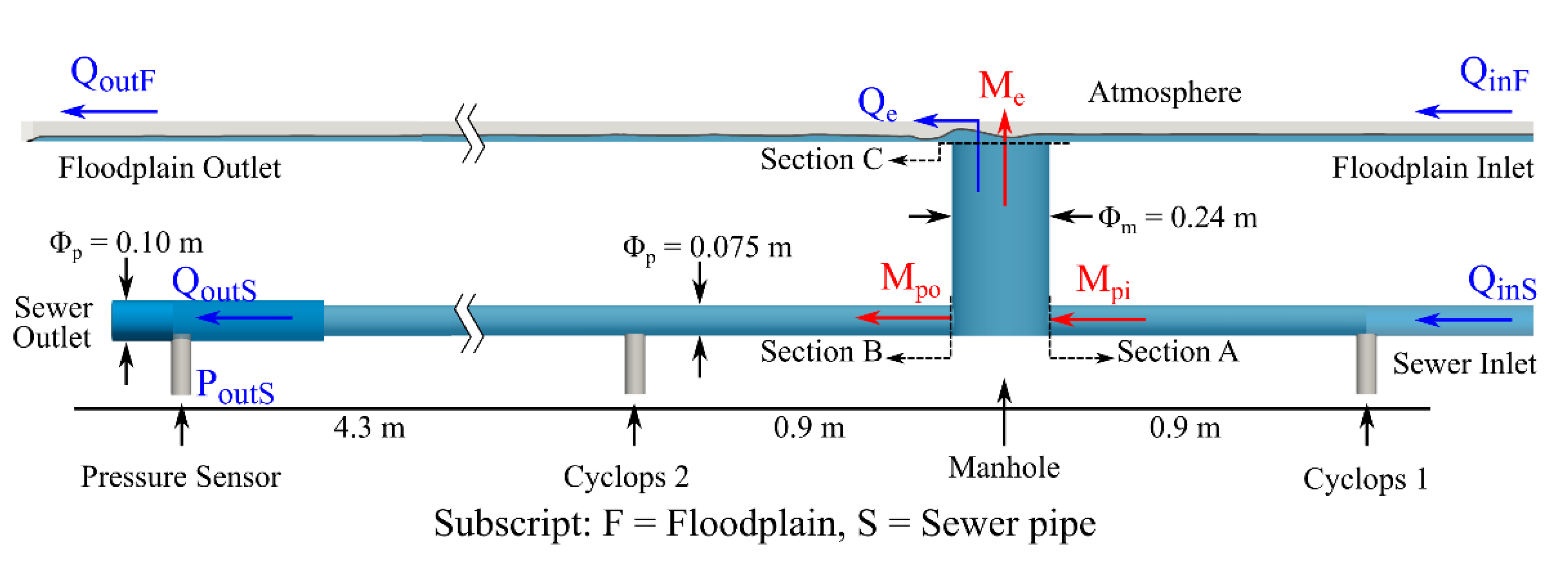
To collect data required for evaluating the numerical model, an experimental testing campaign was conducted using a physical 1:6 scaled model of a linked sewer/surface system, constructed at the University of Sheffield (Figure 1) [11,19,26,27,28,29,30,31]. The model is composed of a surface “floodplain” 8.2 m long, 4 m wide, constructed from acrylic (slope of 0.001 m/m). This floodplain is connected to a piped sewer system via a manhole with a diameter of 0.240 m (simulating a 1.440 m manhole at full scale, a size typical of UK urban drainage systems for pipes diameters up to 900 mm [32]). The sewer comprises a 0.075 m (internal) diameter clear acrylic pipe (simulating a 0.450 m pipe at full scale). To simulate flooding conditions, a series of steady flows were passed into the inlets at the upstream boundary of the sewer system and the floodplain. During each test, a portion of the flow within the piped network passed into the surface system via the manhole structure, with the remaining flow passing to the pipe outlet tank via the downstream boundary. The scheme of the facility is displayed in Figure 1.

The experimental facility was equipped with three electromagnetic flowmeters (two of them at the sewer and surface flow inlet—$Q_{InS}$ and $Q_{InF}$—and one in the outlet of the sewer—$Q_{OutS}$) of 0.075 m internal diameter. The accuracy of the flow meters was validated using volumetric discharge readings at the laboratory measurement tank. A butterfly flow control valve was fitted to the pipe that feeds the sewer and the floodplain, calibrated such that steady inflows from 1 to 11 L/s can be set. Electromagnetic flowmeters and butterfly valves were monitored and controlled via Labview™ software. For all the tests conducted, flows were first established and allowed to stabilise before data values were recorded. Once established, data were collected for a period of 3 min to define reliable temporally averaged values for each flow mater. Mean steady state flow exchange rate through the manhole structure ($Q_e$) was quantified based on mass conservation principles (i.e., $Q_e=Q_{InS}-Q_{OutS}$). During the experimental campaign, water column pressure at the sewer outlet point was measured using pressure sensor (Figure 1). This sensor was calibrated to directly convert the output signal (mA) to gauge pressure and this procedure was conducted using a pointer gauge. The measure values were compared against defined calibration outcomes and errors were quantified to be ±0.69 mm within the water depth range of 0 to 600 mm. Values recorded with the pressure sensor were then gathered in real time by using the same Labview™ software described previously.

Experiments to understand solute transport and mass exchange were undertaken by injection of a neutrally buoyant soluble fluorescing dye (Rhodamine WT) into the sewer pipe >8 m upstream of the first measurement point (Cyclops 1 in Figure 1). The distance between the location of the injection and the measurement areas was higher than 10D (D = sewer pipe diameter) to allow cross sectional mixing [33]. Measurement of concentration vs. time profiles upstream and downstream of the manhole was conducted using Cyclops-7F™ fluorimeters. For this experiment, dye of concentration 10⁻³ mg/L was fed into a constant head tank, from where injection into the sewer pipe was controlled by a manual open/close valve. For each test conducted, a 15 s duration pulse of dye of was introduced into the inflow pipe, and the resulting in-pipe concentrations monitored using the fluorimeters. The electrical sensor output was converted to concentration using experimentally predetermined calibration equations.

Experimental tests were conducted under steady state hydraulic conditions over a range of sewer inflows ($Q_{InS}$) and surface inflows ($Q_{InF}$), producing different flow exchange rates ($Q_e$). Reynolds number (Re) for these tests ranged from 1.37 × 10⁶ to 1.72 × 10⁶ in the sewer inlet, which indicates a fully turbulent flow condition. Surface flow depths measured 350 mm upstream of the centreline of the manhole ranged between 5 to 17 mm over the tests conducted. Full details of these test conditions along with their numerical replication in CFD are presented in Table 1 in Section 3.

2.2. Timescales and Mass Exchange Processes

For a given pulse of soluble contaminant passing within a pipe network entering an exchange structure (e.g., a manhole) during sewer-to-surface flow exchange conditions (i.e., $Q_e$ > 0), a proportion will pass through the structure remaining within the pipe network and a proportion will exit to the surface flow. The change in total solute mass within the exchange structure at a given point in time can be expressed as

$$\frac{d{M}_m}{dt}={\dot{M}}_{PI}-{\dot{M}}_e-{\dot{M}}_{PO}$$

(1)

where $\frac{d{M}_m}{dt}$ is the rate of change in mass of solute within the exchange structure (mg/s), ${\dot{M}}_{PI}$ is the solute mass flow rate entering the exchange structure via the pipe network (mg/s), ${\dot{M}}_e$ is solute mass flow rate (mg/s) leaving the exchange structure to the surface flow and ${\dot{M}}_{PO}$ is the solute mass flow rate leaving the exchange structure via the pipe network (mg/s).

Considering the arrival of a well-mixed solute of concentration (C_PI) at the inlet to the exchange structure under steady inflow conditions and Equation (1) above, a number of characteristic timescales can be defined.

• From time t_o to t₁, solute mass is entirely stored within the exchange structure (prior to solute reaching an exit), thus ${\dot{M}}_e={\dot{M}}_{PO}=0$.
• Assuming typical dimensions and flow conditions encountered within urban drainage exchange structures such as manholes, between t₁ and t₂, solute mass initially leaves the exchange structure via the outlet pipe only, hence ${\dot{M}}_e=0$.
• Between t₂ and t₃ solute mass leaves the exchange structure via the pipe outlet and to the surface, solute mass flow rate to the surface will be dependent on the hydraulic characteristics and evolution of solute inside the exchange structure and all terms in (1) should be considered.
• After t₃ concentration gradients within the structure will have significantly reduced and hence steady mass flow conditions in the structure are achieved, $\frac{d{M}_m}{dt}=0$. Considering that the solute mass flow through an inlet/outlet is a product of the rate of hydraulic flow rate and mean solute concentration, the proportion of solute mass exchanging though each outlet will become equivalent to the flow partition through the structure (Equations (2) and (3)).

$$\frac{{\dot{M}}_e}{{\dot{M}}_{PI}}=\frac{Q_e}{Q_{PI}}$$

(2)

$$\frac{{\dot{M}}_{PO}}{{\dot{M}}_{PI}}=\frac{Q_{PO}}{Q_{PI}}$$

(3)

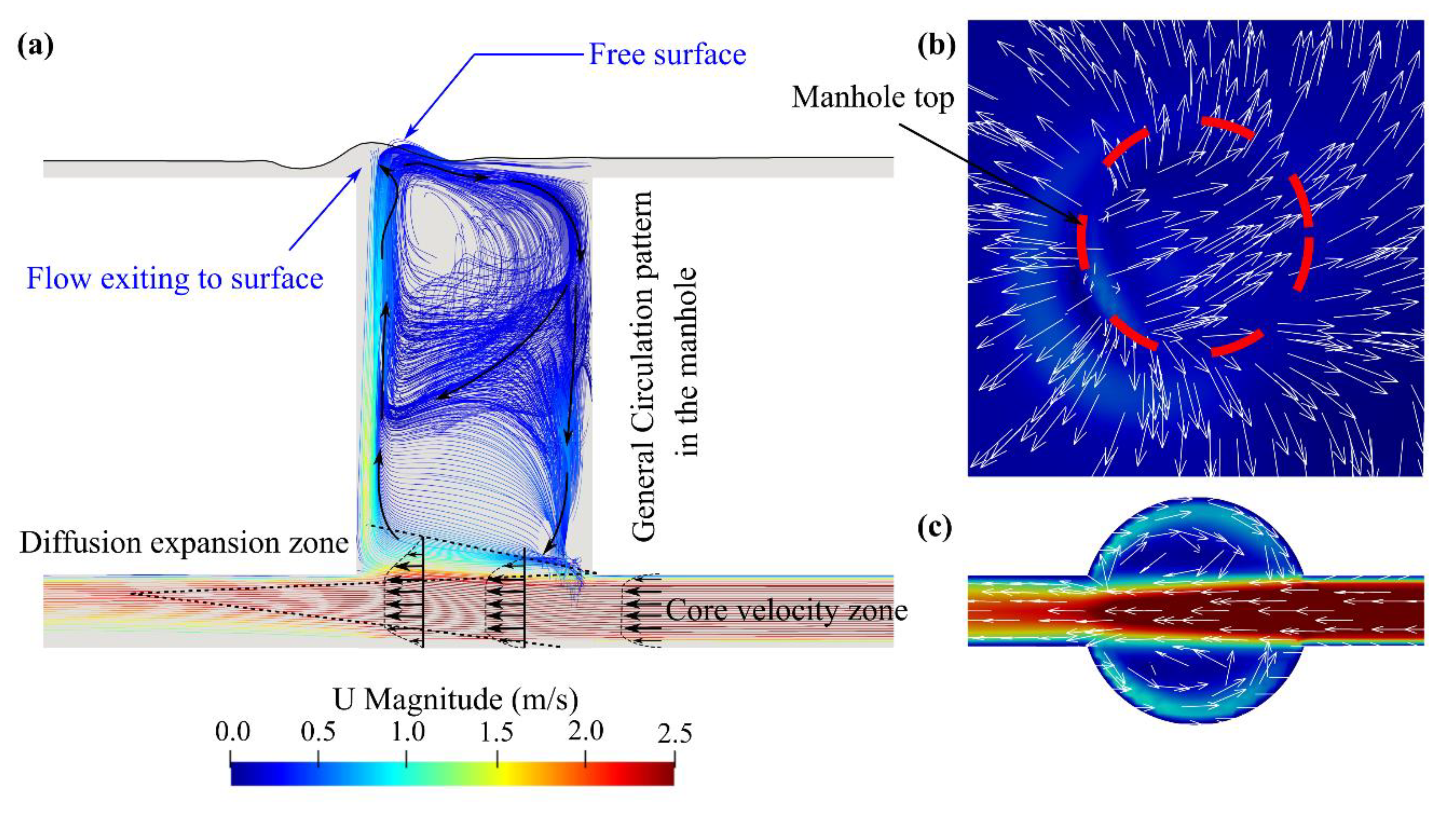
Further experiments on specific hydraulic structures are required to understand the characteristic timescales (t_1,2,3) and how these are affected by local flow characteristics. Flow structures and mixing processes in tanks and urban drainage structures have been studied previously but in the absence of surface flow interaction. For example, a general description of flow structures inmanholes under surcharged pipe conditions is given in [12]. When the sewer pipe inflow enters the manhole, three distinguished flow zone can be commonly observed [12,23,34]. A part of the pressurised flow, known as the diffusion zone, expands inside the manhole at a ratio of 1:5 towards the manhole diameter length. The remaining strong velocity zone forms a conical shape which has the same central axis as the inlet pipe. The slope of this cone is generally 1:6.2 towards the manhole length and travels through the manhole diameter towards the outlet. This conical form may create different distinctive scenarios based on the manhole to sewer pipe diameter ratio (${\varphi }_m$/${\varphi }_m$) and available surcharge depth (s). For 3.0 < ${\varphi }_m/{\varphi }_p$ < 4.5 and with s > 0.2${\varphi }_m$, the core velocity region travels out of the manhole without contributing to the mixing process [23,35]. This is the most conventional size and surcharge depth characteristics for an overflowing manhole commonly seen the drainage systems and corresponds to the present study. In these cases, the diffusion zone is mainly responsible for solute mixing inside a manhole [20,23]. Part of the diffusion zone interacts with the manhole wall and travels upward. Later, this upward moving flow further divides in two components of which the first part exits through the surface and the last part recirculates within the manhole. However, how these structures interact with a surface flow, how effective they are in transporting solute mass to the surface and key timescales for well-mixed conditions (i.e., Equations (2) and (3)) are currently unclear and will be analysed in the current work using CFD techniques.

2.3. CFD Modelling

The hydraulics of the experimental model was reproduced using three-dimensional CFD modelling tools OpenFOAM^® v.18.12 within interFoam solver [36,37,38], which considers the two-fluid system as isothermal, incompressible and immiscible utilising a Volume of Fluid (VOF) model [39]. Despite Larger Eddy Simulation (LES) models being known to model the turbulence structures of the flow more effectively, LES models are significantly more computationally expensive than those of RANS models. Moreover, RANS models are also reported in the literature for their accuracy in replicating manhole hydraulics properly and efficiently [29,34,40]. The model uses a single set of Navier–Stokes equations (Equations (4) and (5)) for both fluids with additional equations to describe the free-surface (Equation (6)). The interFoam within RNG k-ε Reynolds-averaged Navier–Stokes equations also requires Equations (7) and (8).

$$\nabla .\mathit{u}=0$$

(4)

$$\frac{\partial \rho \mathit{u}}{\partial t}+\nabla .\left(\rho \mathit{u}\mathit{u}\right)=-\nabla p^{*}+\nabla .\mathit{\tau }-\mathit{g}.\mathit{x}\nabla \rho +{\mathit{f}}_{\mathit{\sigma }}$$

(5)

$$\frac{\partial \alpha }{\partial \mathrm{t}}+\nabla ·\left(\alpha \mathit{u}\right)+\nabla .\left[{\mathit{u}}_{\mathrm{c}}\alpha \left(1-\alpha \right)\right]=0$$

(6)

$$\frac{\partial \rho k}{\partial \mathrm{t}}+\nabla ·\left(\rho k\mathit{u}\right)=\nabla ·\left({\Gamma }_k\nabla k\right)+P_k-Y_k$$

(7)

$$\frac{\partial \rho \epsilon }{\partial \mathrm{t}}+\nabla ·\left(\rho \epsilon \mathit{u}\right)=\nabla ·\left({\Gamma }_{\epsilon }\nabla \epsilon \right)+P_{\epsilon }-Y_{\epsilon }+D_{\epsilon }$$

(8)

Where $\mathit{u}$ is the mean velocity vector in the Cartesian coordinate; $\rho$ is the density of the fluid mix; $\mathit{g}$ is the acceleration due to gravity; $t$ is the time; $\mathit{\tau }$ is the shear stress tensor; $p^{*}$ is the modified pressure adapted by removing the hydrostatic pressure from the total pressure; ${\mathit{f}}_{\mathit{\sigma }}$ is the volumetric surface tension force (where CSF and interface curvature are included); $\alpha$ is the VOF function; k is the turbulent kinetic energy; $\epsilon$ is the energy dissipation; ${\Gamma }_k$ and ${\Gamma }_{\epsilon }$ are the diffusion for $k$ and $\epsilon$, respectively; and P, Y and D are the Production, Dissipation and Additional term for RNG, respectively.

In this work, an additional solute transport model was added to the interFoam VOF model. The main advection–dispersion equation used in the model is

$$\frac{\partial \mathrm{c}}{\partial \mathrm{t}}+\nabla .\left(\mathit{u}-v_s\frac{\mathit{g}}{\left|\mathit{g}\right|}\right)c=\nabla .\left(\alpha {\nu }_t\nabla c\right)$$

(9)

where $c$ is the solute concentration of the flow, $v_s$ is the terminal velocity due to gravity (which is zero for a neutrally buoyant solute) and ${\nu }_t$ is the turbulent kinematic viscosity of water, which is a function of the turbulence of the flow [41] and taken to be equivalent to diffusivity [42,43]. The multiplication of ${\nu }_t$ by $\alpha$ prevents solute particles from entering the air phase [42].

Earlier model validation works by the authors presenting measured velocities using PIV within the same experimental facility [29] showed that RNG k-ε model is a suitable RANS modelling choice for predicting water elevation and velocity profiles and hence is chosen for this work. This turbulence model can also capture complex flow and is known for better performance for separating flow [22,23,29]. Apart from wall boundary condition, five open boundaries were prescribed in the model: two inlet and two outlet boundaries at the sewer pipe and floodplain, respectively, and an atmosphere boundary at the floodplain (Figure 1). The inlet boundaries were prescribed as fixed velocities, while the outlets were applied as fixed pressure. This measured temporal mean pressure data was used for the sewer outlet pressure boundary condition (measured at $P_{OutS}$). The atmosphere boundary was set as equal to atmospheric pressure and zero gradient for velocity to have free airflow if required. All the wall boundaries were prescribed as noSlip condition. The sewer pipe walls were considered as rough wall applying equivalent sand roughness height (ks). Further details of measured head losses within the experimental facility can be found in [26].

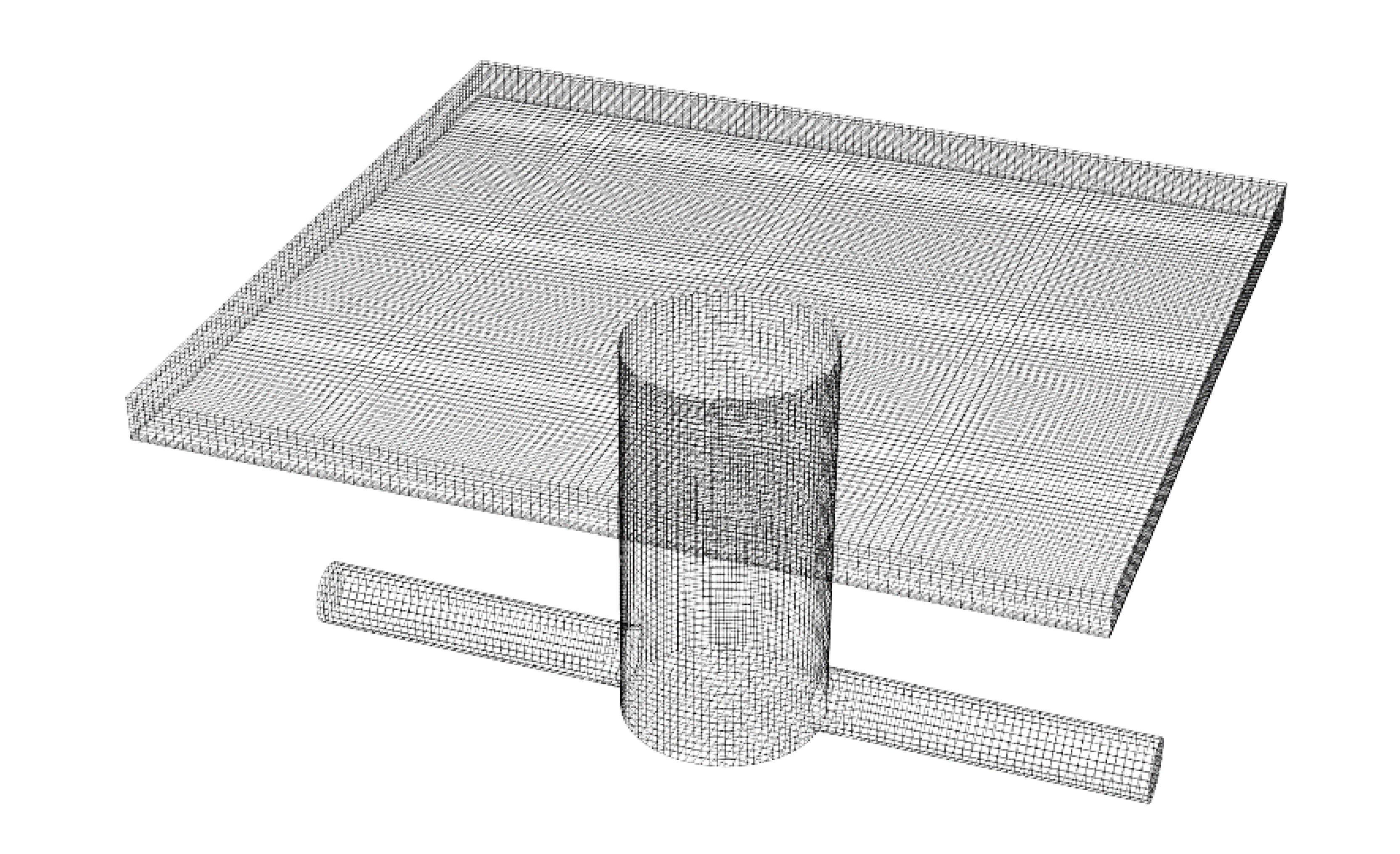
Cfmesh v1.1 [44] was used to generate the hexahedral computational meshes, keeping the maximum mesh size as 10 mm towards all three Cartesian directions. The boundary meshes were kept small in such a way that 30 < y⁺ < 300, keeping three boundary layers at the all wall boundaries. A standard wall function was applied to all the walls, which has been shown to be appropriate for the application of boundary turbulence effects for such mesh sizes [36], eliminating the necessity of fine layered boundary meshes. Figure 2 shows part of the computational mesh created for this work. The rest of the CFD model such as the choice of different meshes, different solvers parameters and solution schemes were obtained from another CFD model validated in an earlier work depicting the same experimental set-up [23,29]. The maximum Courant–Friedrichs–Lewy (CFL) number was kept as 0.9. The cluster computing system at the University of Coimbra was used to run the simulations using MPI mode. Each simulation was run for 300 s to reach steady state conditions. For comparisons with experimental datasets, the measured solute concentration for each test condition was applied through the sewer inlet pipe at Cyclopes 1 when the hydraulic model reached a steady state. Unsteady model results were saved at every 0.01 s interval. Model solute concentrations were extracted at different sections and compared with the experimental measurements.

Experimental tests 1–6 (including repeats) listed in Table 1 were replicated to perform calibration and testing of the CFD model. In these tests, solute concentration in the inflow pipe was taken as the measured value recorded at Cyclopes 1. Measured and predicted concentration curves are compared at the downstream measurement point (Cyclopes 2) along with measured and modelled flow rates in the pipe and exchanging to the surface (i.e., flow partition).

To isolate and understand the effects of the manhole separately from the pipe network, the calibrated model was further applied to Test 1-A, 2-A, 3-A and 4-A under identical hydraulic conditions to tests 1, 2, 3 and 4, respectively. However, in these tests, solute concentration was applied uniformly at the sewer pipe/manhole inlet boundary at a steady concentration of 1.2 × 10⁻⁶ mg/L. Resulting concentration time series were extracted at the manhole–pipe junctions (section A and B in Figure 1) and at the exit to the surface flow (section C in Figure 1). Solute mass flow rates to the surface flow and the downstream pipe as well as characteristic time scales of the manhole as described in Section 2.1 were calculated from these tests (described further in Section 3.3). Test 1 was further extended numerically by changing the downstream boundary pressure; by decreasing 9.5% (Test 1-B) and by increasing 15% (Test 1-C) to enable lower and higher pipe to surface exchange flows (1.21 L/s and 2.43 L/s), respectively.

3. Results

3.1. Model Calibration and Validation—Hydrodynamics

Calibration of wall roughness (ks) was performed based on experimental test results of flow exchange through the manhole to the surface. Applying a higher ks in the sewer pipe leads to lower flow through the outlet pipe with higher flow exchange from the manhole to the surface, and vice versa. The experimental values from Test 4 were used for calibration purposes as it had a sewer inlet flow which was median to all the sewer flows tested herein. Modelled ks values ranging from 1 × 10⁻⁶ to 1 × 10⁻³ mm were simulated in the CFD model. Results showed that ks = 0.0005 mm gives a comparable modelled value of the flow partition to the experimentally observed values ($Q_e$ within 1.7%). This value of ks is valid for smooth surfaces such as acrylic which is appropriate to the experimental setup used here. The same ks value was applied to the rest of the hydraulic simulations (Tests 1–3 and 5–6) for model validation. Table 1 compares experimentally measured and modelled steady state flow rates in the pipe and exchanged to the surface ($Q_{OutS}$ and $Q_e$) for each test, along with measured boundary conditions and calculated Reynolds numbers. Modelled and measured flow rates are found to be within 1.7% in all cases. Figure 3 presents resulting calculated velocity streamlines and vectors within the manhole during Test 4.

Table 1. Experimentally observed and numerical flow rates for each test case. Solute injections for tests 4–6 were repeated 3 times.

Test ID	Boundary Condition			Experimental		Numerical		Experimental Reynold’s No.		$\%\mathbf{of}\mathbf{Diff}.\mathbf{in}{\mathit{Q}}_{\mathit{e}}$
	$$\begin{gathered} \mathbf{U}/\mathbf{S}{\mathit{Q}}_{\mathit{I}\mathit{n}\mathit{F}} \\ (\mathbf{L}/\mathbf{s}) \end{gathered}$$	$$\begin{gathered} \mathbf{U}/\mathbf{S}{\mathit{Q}}_{\mathit{I}\mathit{n}\mathit{F}} \\ (\mathbf{L}/\mathbf{s}) \end{gathered}$$	$\mathbf{D}/\mathbf{S}{\mathit{P}}_{\mathit{o}\mathit{u}\mathit{t}\mathit{S}}\left(\mathbf{mm}\right)$	${\mathit{Q}}_{\mathit{O}\mathit{u}\mathit{t}\mathit{S}}(\mathbf{L}/\mathbf{s})$	${\mathit{Q}}_{\mathit{e}}(\mathbf{L}/\mathbf{s})$	${\mathit{Q}}_{\mathit{O}\mathit{u}\mathit{t}\mathit{S}}(\mathbf{L}/\mathbf{s})$	${\mathit{Q}}_{\mathit{e}}(\mathbf{L}/\mathbf{s})$	Inlet Sewer	Outlet Sewer
Test 1	4.28	8.09	415.9	6.42	1.67	6.44	1.65	137020	108680	1.20
Test 2	4.28	9.00	428.3	6.84	2.17	6.84	2.16	152480	115790	0.46
Test 3	4.28	9.67	436.7	7.18	2.49	7.14	2.53	163830	121620	1.61
Test 4 *	6.29	10.20	448.7	6.72	3.48	6.66	3.54	172710	113830	1.72
Test 5	7.46	10.20	450.2	6.70	3.50	6.65	3.55	172710	113490	1.43
Test 6	8.64	10.19	447.5	6.67	3.52	6.66	3.53	172710	112980	0.28

* Test 4 data was used for hydraulic calibration.

Table 1. Experimentally observed and numerical flow rates for each test case. Solute injections for tests 4–6 were repeated 3 times.

Test ID	Boundary Condition			Experimental		Numerical		Experimental Reynold’s No.		$\%\mathbf{of}\mathbf{Diff}.\mathbf{in}{\mathit{Q}}_{\mathit{e}}$
	$$\begin{gathered} \mathbf{U}/\mathbf{S}{\mathit{Q}}_{\mathit{I}\mathit{n}\mathit{F}} \\ (\mathbf{L}/\mathbf{s}) \end{gathered}$$	$$\begin{gathered} \mathbf{U}/\mathbf{S}{\mathit{Q}}_{\mathit{I}\mathit{n}\mathit{F}} \\ (\mathbf{L}/\mathbf{s}) \end{gathered}$$	$\mathbf{D}/\mathbf{S}{\mathit{P}}_{\mathit{o}\mathit{u}\mathit{t}\mathit{S}}\left(\mathbf{mm}\right)$	${\mathit{Q}}_{\mathit{O}\mathit{u}\mathit{t}\mathit{S}}(\mathbf{L}/\mathbf{s})$	${\mathit{Q}}_{\mathit{e}}(\mathbf{L}/\mathbf{s})$	${\mathit{Q}}_{\mathit{O}\mathit{u}\mathit{t}\mathit{S}}(\mathbf{L}/\mathbf{s})$	${\mathit{Q}}_{\mathit{e}}(\mathbf{L}/\mathbf{s})$	Inlet Sewer	Outlet Sewer
Test 1	4.28	8.09	415.9	6.42	1.67	6.44	1.65	137020	108680	1.20
Test 2	4.28	9.00	428.3	6.84	2.17	6.84	2.16	152480	115790	0.46
Test 3	4.28	9.67	436.7	7.18	2.49	7.14	2.53	163830	121620	1.61
Test 4 *	6.29	10.20	448.7	6.72	3.48	6.66	3.54	172710	113830	1.72
Test 5	7.46	10.20	450.2	6.70	3.50	6.65	3.55	172710	113490	1.43
Test 6	8.64	10.19	447.5	6.67	3.52	6.66	3.53	172710	112980	0.28

* Test 4 data was used for hydraulic calibration.

Figure 3. Hydraulic conditions inside the manhole during Test 4. (a) Streamline of the flow indicating a general circulation pattern, (b) mean velocity vectors at the top horizontal plane of the manhole and (c) mean velocity vectors at the horizontal plane passing through the sewer pipe axis of the manhole. At all cases, main flow direction is from right to the left.

Figure 3. Hydraulic conditions inside the manhole during Test 4. (a) Streamline of the flow indicating a general circulation pattern, (b) mean velocity vectors at the top horizontal plane of the manhole and (c) mean velocity vectors at the horizontal plane passing through the sewer pipe axis of the manhole. At all cases, main flow direction is from right to the left.

3.2. Model Replication of Mixing Processes within the Manhole

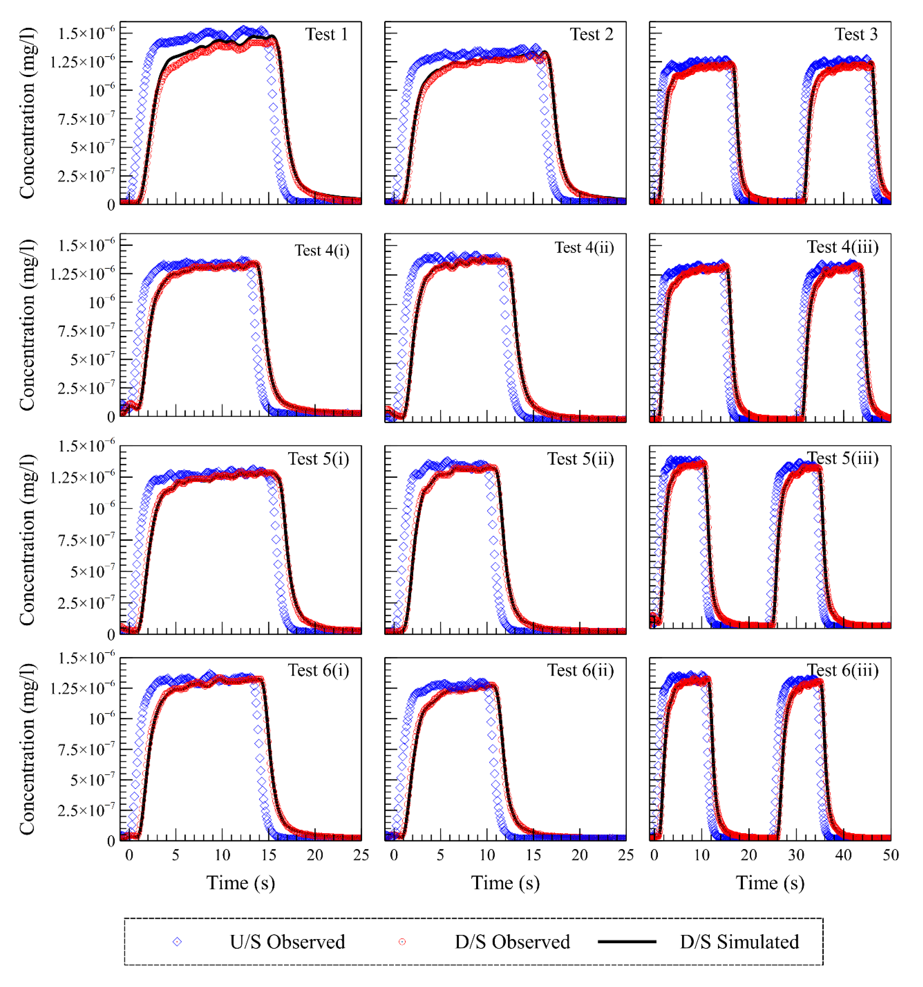
Following validation of the hydrodynamic processes, the ability of the CFD model to simulate solute mixing within the manhole was tested by comparing measured and simulated concentration profiles within the pipe network (at the location of Cyclopes 2) for all hydraulic conditions. Solute injections for hydraulic conditions in Tests 1–3 were performed once using either a single or double pulse of solute concentration. Injections during hydraulic conditions in Tests 4–6 were repeated three times each, of which the first two had single pulse and the third had two consecutive concentration pulses. Measured and predicted solute concentration time series at manhole D/S (at the location of Cyclopes 2) were extracted compared to those of experimental data. Figure 4 shows comparison of experimentally measured and modelled concentration time series at the manhole downstream measurement point for each test.

Different statistical parameters were used to check the quality of model performance in predicting the solute concentration at the downstream of the manhole. The parameters used are listed below.

• Average of error, $BIAS=\frac{1}{n}{\displaystyle \sum }_{i=1}^n\left(O_i-P_i\right)$
• Root mean square error, $RMSE=\frac{1}{n}\sqrt{{\displaystyle \sum }_{i=1}^n{\left(O_i-P_i\right)}^2}$
• Pearson product-moment correlation coefficient, $r=\frac{{{\displaystyle \sum }}_{i=1}^n\left(O_i-\overline{O}\right)\left(P_i-\overline{P}\right)}{\sqrt{{{\displaystyle \sum }}_{i=1}^n{\left(O_i-\overline{O}\right)}^2{\left(P_i-\overline{P}\right)}^2}}$
• Nash Sutcliffe coefficient, $NSC=1-\frac{{{\displaystyle \sum }}_{i=1}^n{\left(O_i-P_i\right)}^2}{{{\displaystyle \sum }}_{i=1}^n{\left(O_i-\overline{O}\right)}^2}$

Where $O_i$ is the observation values, $P_i$ is the model predicted values, and $\overline{O}$ is the average of all observed values, $\overline{P}$ is the average of model predicted values and $n$ is the number of observations. The calculated values of the mentioned statistical parameters are shown in

Table 2. Statistical comparisons between the concentration time series between experimental and numerical models.

Test ID	BIAS (mg/L)	RMSE (mg/L)	r	NSC
Test 1	−3.89 × 10−8	4.46 × 10−8	1.000	0.995
Test 2	−2.48 × 10−8	2.78 × 10−8	1.000	0.997
Test 3	−1.39 × 10−8	1.87 × 10−8	1.000	0.999
Test 4 (i)	3.41 × 10−9	1.45 × 10−8	1.000	0.999
Test 4 (ii)	2.53 × 10−9	1.27 × 10−8	1.000	1.000
Test 4 (iii)	4.70 × 10−9	1.90 × 10−8	0.999	0.999
Test 5 (i)	3.68 × 10−9	2.28 × 10−8	1.000	0.999
Test 5 (ii)	3.62 × 10−9	2.69 × 10−8	1.000	0.998
Test 5 (iii)	4.55 × 10−9	1.25 × 10−8	1.000	1.000
Test 6 (i)	5.01 × 10−9	2.59 × 10−8	1.000	0.999
Test 6 (ii)	3.03 × 10−9	2.62 × 10−8	1.000	0.998
Test 6 (iii)	6.57 × 10−9	2.97 × 10−8	0.999	0.997

. It shows that BIAS of all the comparisons is negligible. The NSC values are greater than 0.995 in all cases. Therefore, the results show that the model accurately replicates the solute mixing processes within the manhole.

3.3. Modelling of Soluble Mass Exchange to Surface Flows

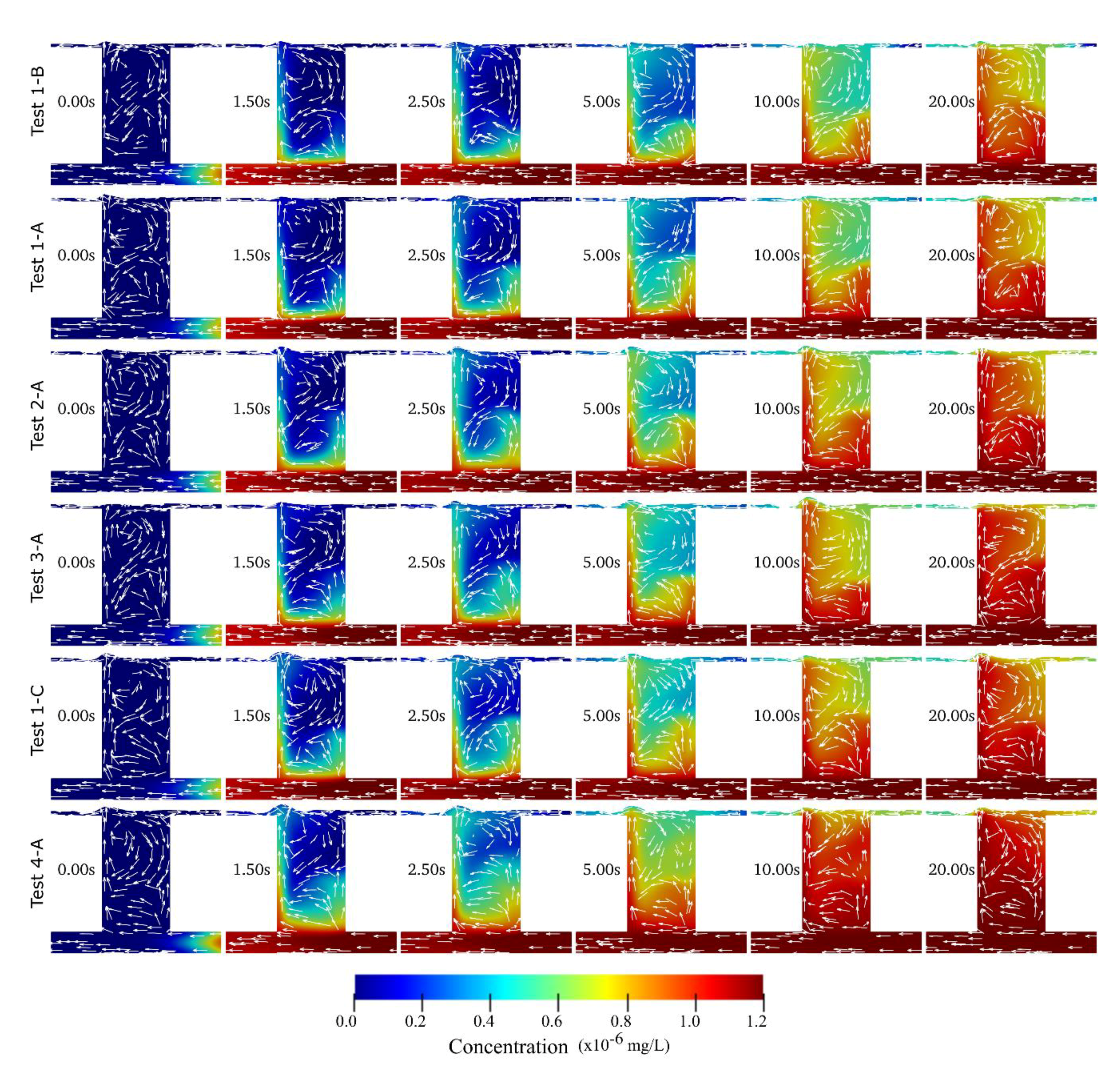
The solute transport model was then applied to Test 1-A-B-C, 2-A, 3-A and 4-A, as described in Section 2.3 (i.e., with a uniform solute applied directly to the manhole inlet boundary at Section A). Figure 5 shows example plots of concentration evolution inside the manhole for each of these tests at different time intervals. Time t₀ = 0 is taken when average solute concentration at Section A exceeds 1% of the peak value. Instantaneous velocity vectors are also displayed to indicate the travel paths of the solute concentration within the manhole volume.

Figure 5 shows that as soon as the solute mass enters the manhole, it diffuses from the high velocity flow region into the manhole volume. A part of the concentrated solute mass hits the opposite manhole wall and travels towards the manhole surface. Later, it interacts with the surface flow and recirculates to the manhole. This recirculating flow brings low concentration flow from the surface into the manhole, maintaining a consistent concentration gradient through the manhole height until the upper part becomes completely mixed. The observed flow structures explored in the tests are relativity insensitive to the pipe inflow rate over the partition ratios used in these tests. The results show that until well mixed conditions are achieved, that the concentration field at the manhole/surface interaction point (section C) is highly heterogeneous. Therefore unlike in the pipe network, (where cross-sectionally averaged values can be reasonably assumed at Sections A and B), quantification of mass flow rate to the surface (i.e., over Section C) requires robust understanding of the spatial variation of solute and velocity over the manhole cross section and how this evolves with time.

The evolution of solute mass exchange through each cross section A, B and C is quantified based on the CFD model. For this purpose, CFD model results of test 1-A-B-C, 2-A, 3-A and 4-A were considered. Due to highly heterogeneous conditions at section C, mass flow rate at each time step for each inlet/outlet junctions (section A, B, C) was calculated using the following Equation,

$${\dot{M}}_x={{\displaystyle \int }}_{i=0}^{i=A}{c}_i{\mathit{u}}_{i}d\mathit{A}$$

(10)

where ${\dot{M}}_x$ is the solute mass flow rate though section A, B or C (i.e., ${\dot{M}}_{PI},{\dot{M}}_e$ or ${\dot{M}}_{PO}$); ${\mathit{u}}_i$ is the mean velocity vector normal to area i; $d\mathit{A}$ is an incremental cross section area vector (based on a 10mm slice); and $c_i$ is the solute concentration within area i. Hence the integral value of the dot multiplication of these components is used to provide the net mass flow rate through sections A, B and C. The model set-up (uniform concentration applied at Section A) results in a constant ${\dot{M}}_{PI}$ over each test after the first 0.2 s of simulation (as given in

Table 3. Characteristic time scales of solute mixing from different model results. Results are arranged in an ascending order of the mean surface flow partition ratios.

Test ID	$\mathbf{Inlet}\mathbf{Mass}\mathbf{Flowrate},{\dot{\mathit{M}}}_{\mathit{P}\mathit{I}}$(×10−6 mg/s)	Nominal Residence Time, Tx (s)	Mean Surface Flow Partition Ratio $({\mathit{Q}}_{\mathit{e}}/{\mathit{Q}}_{\mathit{i}\mathit{n}\mathit{S}})$	Non-Dimensional Characteristic Time (-)			Fitted Curve Coefficients
				t1/Tx	t2/Tx	t3/Tx	C	r2
1-B	9.7	4.09	0.150	0.03	0.20	5.80	0.35	0.9071
1-A	9.7	2.96	0.206	0.04	0.27	8.11	0.40	0.9677
2-A	10.8	2.28	0.241	0.05	0.34	8.27	0.40	0.9455
3-A	11.6	1.99	0.257	0.05	0.25	9.20	0.45	0.9545
1-C	9.7	2.24	0.302	0.05	0.26	9.79	0.52	0.9797
4-A	12.3	1.42	0.342	0.06	0.28	9.55	0.60	0.9356

). Following the calculation of ${\dot{M}}_{PI},{\dot{M}}_e$ and ${\dot{M}}_{PO}$, the rate of change in solute mass within the manhole was calculated using Equation (1). Figure 6 shows resulting outlet solute mass flow rates as a ratio of manhole inlet mass flow rate over each test. The time axis in the figures represents time (in seconds) since the first solute enters the manhole from the sewer inlet. As in Figure 5, this time (t₀ = 0) is taken when average solute concentration at Section A exceeds 1% of the peak value. Significant fluctuation can be observed in the $\frac{{\dot{M}}_e}{{\dot{M}}_{PI}}$ values due to the complex heterogeneous nature of the flow at the surface/manhole interaction point (section C).

Characteristic time scales, as described in Section 2.2, are defined for each test and are presented in Table 3. Similar to the definition of t₀, t₁ and t₂ are taken when averaged solute concentration at Sections B and C exceeds 1% of the peak value, respectively. t₃ is defined as the time when $\frac{d{M}_m}{dt}$ falls below 2.5% of its peak value for the first time. Timescales in Table 3 are presented non-dimensionally in terms of the nominal manhole residence time for flow passing to the surface $T_x$, as calculated using Equation (11),

$$T_x=\frac{L_x\frac{\pi }{4}{\left({\mathsf{\Phi }}_m\right)}^2}{Q_e}$$

(11)

where $L_x$ is the vertical distance between the sewer pipe axis and the manhole top and ${\mathsf{\Phi }}_m$ is the manhole cross sectional area.

As can be seen in Figure 6a,b, for each test the proportion of mass flow rate entering the pipe outlet ($M_{PO}/M_{PI}$) and surface flow ($M_e/M_{PI}$) grows asymptotically toward the relevant flow partition ratio (as defined in Equations (2) and (3)). Therefore, solute mass flow exchange to the surface can be described using the following function,

$$\frac{M_e}{M_{Pin}}=\left(\frac{-1}{C\left(t-t_2\right)+1}+1\right)\frac{Q_e}{Q_{inS}}$$

(12)

where C is an empirical coefficient. The best fit value of C and resulting goodness of fit (r²) value between fitted equation and CFD model results for each test conducted in this work is given in Table 3. The first arrival of mass at the pipe exit (t₁) and the surface flow (t₂) occurs relatively quickly in all conditions (0.09 s < t₁ < 0.13 s and 0.40 s < t₂ < 0.82 s), while the timescale for complete mixing (t₃) to be achieved (and thus mass flow rate to the surface flow to become approximately steady and equivalent to the surface flow partition ratio) varies significantly over the tests conducted (13.6 s < t₃ < 24.0 s). From Table 3 the value of C and the non-dimensional timescale (t_1,2,3/T_x) to achieve well mixed conditions tend to increase with the flow partition ratio over the range of conditions tested.

4. Discussion

A comparison of experimentally measured and modelled discharges within a scaled manhole structure shows that, given knowledge of the boundary conditions, the RANS CFD approach accurately simulates flow exchange from piped to surface flows (within 1.7% in all test cases). Therefore, steady-state flow exchange through similar hydraulic structures during flood events is likely to be well described using RANS CFD. These results concur with previous validation studies utilising similar 3D modelling approaches to simulate hydrodynamics in urban drainage structures (see, e.g., in [29,45]), although in this case the complex interaction with surface flows as well as a solute transport is also recreated. Such models are too computationally expensive to be used in direct flood modelling applications; however, there is further potential to utilise such complex models to evaluate simpler semiempirical weir/orifice relationships currently used to describe surface/sewer interaction. Such semiempirical relationships have been found to be sensitive to interaction structure type, inlet characteristics and geometry as well as unsteady hydraulic conditions [12,30,46,47], and thus benefit from case-specific calibration. Similarly, the calibrated model has been shown to accurately reproduce solute concentration profiles (and thus mass flow rates) measured downstream of the manhole structure under a range of flow rates during cases where sewer flow interacts with surface flood water. Taken together with the agreement of modelled and measured flow partition within the manhole, as well as past results comparing CFD velocity vectors against those obtained using PIV measurement in the same facility [29], this result gives confidence that the CFD model can reproduce flow details and resulting solute mass exchange to the surface during flood conditions. A full validation would benefit from having access to measured values of concentration/mass exchange at the interaction point between sewer and surface flows (section C); however, the current results have demonstrated the hydraulic complexity and spatial heterogeneity of concentration at this position. Therefore, such validation measurements would require complex instrumentation such as Laser-Induced Fluorescence (LIF) to provide detailed spatial data over the manhole area. In addition, further validation of CFD approaches would be valuable in more complex hydraulic conditions (e.g., unsteady flow), in systems with different geometrical features or at different scales or in cases involving sediments which are also commonly present in urban drainage networks and may be susceptible to transportation in flood water.

The modelled flow structures illustrate the complexity of the interaction between surcharging manhole flow and surface flood water; however, flow structures within the manhole appear to be relativity insensitive to the pipe inflow rate over the flow partition ratios explored in these tests. The solute transport and resulting mass flow rates within the system are a process of both advection and diffusion. The solute transport from the manhole inlet to the manhole pipe outlet is dominated by the advection process due to the strong local velocities in this zone. Thus, first arrival time to the sewer outlet (t₁) is dominated by the sewer inlet velocity with little subsequent variation within these tests. In addition, as the flow partition ratio increases (i.e., more flow is transported to the surface) the corresponding timescales for first arrival of mass at the surface (t₂) and complete mixing within the manhole (t₃) decrease slightly due to the increasing advection through the manhole structure to the surface. However, a stronger positive relationship is observed between non-dimensional timescales based on the characteristic manhole residence time (t₂/T_x, t₃/T_x) and surface partition ratio ($Q_e/Q_{inS})$, indicating the relative significance of conical flow structures produced by the inlet pipe and subsequent diffusive mixing processes in the tests conducted.

The work has shown that the sharp arrival of a well-mixed solute at an open manhole results in an asymptotic growth of mass exchange to the surface, converging to a value that is defined by the hydraulic flow partition. Parameterisation of an asymptotic growth function (C) may be related to the flow partition ratio and/or the characteristic residence time, with more rapid mixing occurring at lower residence times. Approximately well-mixed conditions (and associated equivalence of sewer to surface solute mass exchange s and flow partition ratios) occur at between 5.8 and 9.2 times the manhole residence time over the conditions tested here. Further work is required to explore these relationships over a range of manhole geometries, using different (time varying) solute injection profiles and unsteady hydraulic conditions as well as in other exchange structures such as gullies featuring grills/covers, including at full scale, such that realistic timescales in real situations can be established. A more complete understanding of this problem should also consider the transport of solids, such as fine sediments and entrained material, which are also present in urban drainage networks. In addition, other flood scenarios (e.g., further exploring the influence of surface flow depth and velocity) and cases where the majority of flow transfers to the surface ($Q_e$/$Q_{inS}$ > 0.5) could be explored. In such cases where the surface flow partition ratio is significantly larger, the bulk advection of solute by the flow is likely to increasingly dominate diffusivity arising from local flow structures.

5. Conclusions

A 3D CFD model was applied to simulate flows in an exchange structure involving interacting pipe and surface flows to quantify flow and soluble pollutant mass exchange. The model was validated with a laboratory-scale model, achieving differences of less than 1.7% in flow rates and excellent statistical comparisons between observed and modelled concentration time series. This suggests that a RANS CFD approach is an appropriate methodology to evaluate flow partition and to evaluate how soluble pollutants move from sewer networks to surface flood flows.

The model was extended to different conditions to understand the effects of the manhole separately from the pipe network, and used to calculate the evolution of solute mass transport rate through each manhole open boundary cross section under a range of flow conditions including interactions between sewer flows and surface flood water. A sharp arrival of solute into the structure is shown to result in an asymptotic growth of solute mass exchange ratio to the surface converging to a value equal to the surface flow partition ratio. An analysis of the results demonstrates that the timescales to achieve this convergence are dependent on the diffusive transport inside the structure.

The work in this paper describes initial steps to understand the risks of soluble material from sewer networks entering urban flood waters via exchange structures. The transport of pollutants through these structures will also depend on additional factors including, but not limited to, the presence of manhole coverings and change of structure geometry/shape. In order to build a more complete understanding, such that risks to public health can be understood and quantified, requires significantly more work. This includes further consideration of transport and transformations of both contaminated sediments and soluble materials in urban drainage networks as well as datasets from urban drainage networks, floodwaters and urban surfaces such that transport, survival and fate can be modelled within quantifiable uncertainty bounds.

References

- Arnell, N.W.; Gosling, S.N. The impacts of climate change on river flood risk at the global scale. Clim. Chang. 2016, 134, 387–401. [Google Scholar] [CrossRef] [Green Version]
- Acquaotta, F.; Faccini, F.; Fratianni, S.; Paliaga, G.; Sacchini, A.; Vilímek, V. Increased flash flooding in Genoa Metropolitan Area: A combination of climate changes and soil consumption? Meteorol. Atmos. Phys. 2019, 131, 1099–1110. [Google Scholar] [CrossRef]
- Rubinato, M.; Nichols, A.; Peng, Y.; Zhang, J.-m.; Lashford, C.; Cai, Y.-p.; Lin, P.-z.; Tait, S. Urban and river flooding: Comparison of flood risk management approaches in the UK and China and an assessment of future knowledge needs. Water Sci. Eng. 2019, 12, 274–283. [Google Scholar] [CrossRef]
- Simões, N.E.; Ochoa-Rodríguez, S.; Wang, L.P.; Pina, R.D.; Marques, A.S.; Onof, C.; Leitão, J.P. Stochastic urban pluvial flood hazard maps based upon a spatial-temporal rainfall generator. Water 2015, 7, 3396–3406. [Google Scholar] [CrossRef]
- Wan Mohtar, W.H.M.; Abdullah, J.; Abdul Maulud, K.N.; Muhammad, N.S. Urban flash flood index based on historical rainfall events. Sustain. Cities Soc. 2020, 56. [Google Scholar] [CrossRef]
- Mort, M.; Walker, M.; Williams, A.L.; Bingley, A. Displacement: Critical insights from flood-affected children. Health Place 2018, 52, 148–154. [Google Scholar] [CrossRef]
- De Man, H.; Van Den Berg, H.H.J.L.; Leenen, E.J.T.M.; Schijven, J.F.; Schets, F.M.; Van Der Vliet, J.C.; Van Knapen, F.; De Roda Husman, A.M. Quantitative assessment of infection risk from exposure to waterborne pathogens in urban floodwater. Water Res. 2014, 48, 90–99. [Google Scholar] [CrossRef]
- Sales-Ortells, H.; Medema, G. Microbial health risks associated with exposure to stormwater in a water plaza. Water Res. 2015, 74, 34–46. [Google Scholar] [CrossRef]
- Ten Veldhuis, J.A.E.; Clemens, F.H.L.R.; Sterk, G.; Berends, B.R. Microbial risks associated with exposure to pathogens in contaminated urban flood water. Water Res. 2010, 44, 2910–2918. [Google Scholar] [CrossRef]
- Collender, P.A.; Cooke, O.C.; Bryant, L.D.; Kjeldsen, T.R.; Remais, J.V. Estimating the microbiological risks associated with inland flood events: Bridging theory and models of pathogen transport. Crit. Rev. Environ. Sci. Technol. 2016, 46, 1787–1833. [Google Scholar] [CrossRef]
- Rubinato, M.; Martins, R.; Kesserwani, G.; Leandro, J.; Djordjević, S.; Shucksmith, J. Experimental calibration and validation of sewer/surface flow exchange equations in steady and unsteady flow conditions. J. Hydrol. 2017, 552, 421–432. [Google Scholar] [CrossRef]
- Beg, M.N.A.; Carvalho, R.F.; Leandro, J. Effect of surcharge on gully-manhole flow. J. Hydro-Environ. Res. 2018, 19, 224–236. [Google Scholar] [CrossRef] [Green Version]
- Carvalho, R.F.; Lopes, P.; Leandro, J.; David, L.M. Numerical research of flows into gullies with different outlet locations. Water 2019, 11, 794. [Google Scholar] [CrossRef] [Green Version]
- Hammond, M.J.; Chen, A.S.; Djordjević, S.; Butler, D.; Mark, O. Urban flood impact assessment: A state-of-the-art review. Urban Water J. 2015, 12, 14–29. [Google Scholar] [CrossRef] [Green Version]
- Mark, O.; Jørgensen, C.; Hammond, M.; Khan, D.; Tjener, R.; Erichsen, A.; Helwigh, B. A New Methodology for Modelling of Health Risk from Urban Flooding Exemplified by Cholera—Case Dhaka, Bangladesh; Blackwell Publishing Inc.: Hoboken, NJ, USA, 2018; Volume 11, pp. 28–42. [Google Scholar]
- Tscheikner-Gratl, F.; Bellos, V.; Schellart, A.; Moreno-Rodenas, A.; Muthusamy, M.; Langeveld, J.; Clemens, F.; Benedetti, L.; Rico-Ramirez, M.A.; de Carvalho, R.F.; et al. Recent insights on uncertainties present in integrated catchment water quality modelling. Water Res. 2019, 150, 368–379. [Google Scholar] [CrossRef]
- Scoullos, I.M.; Adhikari, S.; Lopez Vazquez, C.M.; van de Vossenberg, J.; Brdjanovic, D. Inactivation of indicator organisms on different surfaces after urban floods. Sci. Total Environ. 2020, 704. [Google Scholar] [CrossRef]
- Schreiber, C.; Heinkel, S.B.; Zacharias, N.; Mertens, F.M.; Christoffels, E.; Gayer, U.; Koch, C.; Kistemann, T. Infectious rain? Evaluation of human pathogen concentrations in stormwater in separate sewer systems. Water Sci. Technol. 2019, 80, 1022–1030. [Google Scholar] [CrossRef]
- Martins, R.; Kesserwani, G.; Rubinato, M.; Lee, S.; Leandro, J.; Djordjević, S.; Shucksmith, J.D. Validation of 2D shock capturing flood models around a surcharging manhole. Urban Water J. 2017, 14, 892–899. [Google Scholar] [CrossRef]
- Guymer, I.; Dennis, P.; O’Brien, R.; Saiyudthong, C. Diameter and Surcharge Effects on Solute Transport across Surcharged Manholes. J. Hydraul. Eng. 2005, 131, 312–321. [Google Scholar] [CrossRef]
- Guymer, I.; Stovin, V.R. One-Dimensional Mixing Model for Surcharged Manholes. J. Hydraul. Eng. 2011, 137, 1160–1172. [Google Scholar] [CrossRef]
- Lau, S.D.; Stovin, V.R.; Guymer, I. The prediction of solute transport in surcharged manholes using CFD. Water Sci. Technol. 2007, 55, 57–64. [Google Scholar] [CrossRef] [PubMed]
- Beg, M.N.A.; Carvalho, R.F.; Leandro, J. Effect of manhole molds and inlet alignment on the hydraulics of circular manhole at changing surcharge. Urban Water J. 2019, 16, 33–44. [Google Scholar] [CrossRef]
- Stovin, V.R.; Guymer, I.; Lau, S.-T.D. Dimensionless method to characterize the mixing effects of surcharged manholes. J. Hydraul. Eng. 2010, 136, 318–327. [Google Scholar] [CrossRef]
- Beg, M.N.A. Detailed Uncertainty Analysis of Urban Hydraulic Structures in Large Catchments. Ph.D. Thesis, Department of Civil Engineering, University of Coimbra, Coimbra, Portugal, 2018. [Google Scholar]
- Rubinato, M. Physical scale modelling of urban flood systems. Ph.D. Thesis, Department of Civil and Structural Engineering, University of Sheffield, Sheffield, UK, 2015. [Google Scholar]
- Rubinato, M.; Martins, R.; Shucksmith, J.D. Quantification of energy losses at a surcharging manhole. Urban Water J. 2018, 9006, 1–8. [Google Scholar] [CrossRef] [Green Version]
- Rubinato, M.; Shucksmith, J.; Saul, A.J.; Shepherd, W. Comparison between InfoWorks hydraulic results and a physical model of an Urban drainage system. Water Sci. Technol. 2013, 68, 372–379. [Google Scholar] [CrossRef]
- Beg, M.N.A.; Carvalho, R.F.; Tait, S.; Brevis, W.; Rubinato, M.; Schellart, A.; Leandro, J. A comparative study of manhole hydraulics using stereoscopic PIV and different RANS models. Water Sci. Technol. 2018, 2017, 87–98. [Google Scholar] [CrossRef]
- Rubinato, M.; Lee, S.; Martins, R.; Shucksmith, J.D. Surface to sewer flow exchange through circular inlets during urban flood conditions. J. Hydroinform. 2018, 20, 564–576. [Google Scholar] [CrossRef] [Green Version]
- Martins, R.; Rubinato, M.; Kesserwani, G.; Leandro, J.; Djordjević, S.; Shucksmith, J.D. On the Characteristics of Velocities Fields in the Vicinity of Manhole Inlet Grates During Flood Events. Water Resour. Res. 2018, 54, 6408–6422. [Google Scholar] [CrossRef]
- Defra. Annex B: National Build. Standards Design and Construction of New Gravity Foul Sewers and Lateral Drains Water Industry Act. 1991 Section 106B Flood and Water Management Act. 2010 Section 42; Defra: London, UK, 2011. [Google Scholar]
- Gotfredsen, E.; Kunoy, J.D.; Mayer, S.; Meyer, K.E. Experimental validation of RANS and DES modelling of pipe flow mixing. Heat Mass Transf. 2020, 56, 2211–2224. [Google Scholar] [CrossRef]
- Stovin, V.R.; Bennett, P.; Guymer, I. Absence of a Hydraulic Threshold in Small-Diameter Surcharged Manholes. ASCE J. Hydraul. Eng. 2013, 139, 984–994. [Google Scholar] [CrossRef] [Green Version]
- Mark, O.; Ilesanmi-Jimoh, M. An analytical model for solute mixing in surcharged manholes. Urban Water J. 2017, 14, 443–451. [Google Scholar] [CrossRef]
- Weller, H.G.; Tabor, G.; Jasak, H.; Fureby, C. A tensorial approach to computational continuum mechanics using object-oriented techniques. Comput. Phys. 1998, 12, 620. [Google Scholar] [CrossRef]
- Jasak, H. Error Analysis and Estimation for the Finite Volume Method with Applications to Fluid Flows. Ph.D. Thesis, University of London, London, UK, 1996. [Google Scholar]
- Rusche, H. Computational Fluid Dynamics of Dispersed Two-Phase Flows at High Phase Fractions. Ph.D. Thesis, University of London, London, UK, 2002. [Google Scholar]
- Hirt, C.W.; Nichols, B.D. Volume of fluid (VOF) method for the dynamics of free boundaries. J. Comput. Phys. 1981, 39, 201–225. [Google Scholar] [CrossRef]
- Bennett, P. Evaluation of the Solute Transport Characteristics of Surcharged Manholes using a RANS Solution. Ph.D. Thesis, Department of Civil and Structural Engineering, University of Sheffield, Sheffield, UK, 2012. [Google Scholar]
- Yakhot, V.; Orszag, S.A.; Thangam, S.; Gatski, T.B.; Speziale, C.G. Development of turbulence models for shear flows by a double expansion technique. Phys. Fluids 1992, 4, 1510–1520. [Google Scholar] [CrossRef] [Green Version]
- Jacobsen, N.G. A Full Hydro and Morphodynamic Description of Breaker Bar Development. Ph.D. Thesis, Technical University of Denmark, Lyngby, Denmark, 2011. [Google Scholar]
- Liu, X.; García, M.H. Three-Dimensional Numerical Model with Free Water Surface and Mesh Deformation for Local Sediment Scour. J. Waterw. Port Coast. Ocean Eng. 2008, 134, 203–217. [Google Scholar] [CrossRef]
- Juretić, F. cfMesh User Guide (v1.1); Creative Fields: Zagreb, Croatia, 2015; Volume 6. [Google Scholar]
- Lopes, P.; Leandro, J.; Carvalho, R.F.; Páscoa, P.; Martins, R. Numerical and experimental investigation of a gully under surcharge conditions. Urban Water J. 2015, 12, 468–476. [Google Scholar] [CrossRef]
- Gómez, M.; Russo, B.; Tellez-Alvarez, J. Experimental investigation to estimate the discharge coefficient of a grate inlet under surcharge conditions. Urban Water J. 2019, 16, 85–91. [Google Scholar] [CrossRef]
- Kemper, S.; Schlenkhoff, A. Experimental study on the hydraulic capacity of grate inlets with supercritical surface flow conditions. Water Sci. Technol. 2019, 79, 1717–1726. [Google Scholar] [CrossRef]
Figure 1.
Scheme of the exchange structure showing the floodplain, sewer pipe and the manhole.
Figure 2.
Computational mesh for the study showing the manhole and its connections to sewer pipes and surface.
Figure 4.
Comparison of experimental and numerical unsteady concentration profiles in the sewer pipe downstream of the manhole (Cyclopes 2) and the measured concentration at the upstream of the manhole (Cyclopes 1). Tests 4–6 are repeated three times (i, ii, iii).
Figure 5.
Instantaneous solute concentrations and velocity vectors at the central vertical plane of the manhole from different tests at time (t) from 0–20 s. The arrows are not drawn to scale.
Figure 6.
(a) Mass exchange ratio at the manhole to sewer pipe outlet from different test results. Horizontal lines indicate / values for each test. (b) Mass exchange ratio at the manhole to surface connection with fitted asymptotic trend lines. Horizontal lines indicate / values for each test. (c) Change in solute mass within the manhole.