Tree-Type Irrigation Pipe Network Planning and Design Method Using ICSO-ASV

Abstract

Research on tree-type irrigation pipe networks is an important component of agricultural water-saving projects. The optimal design of tree-type irrigation pipe networks is a key aspect regarding the profitability of irrigated agriculture. Meanwhile, swarm intelligence optimization algorithms have good computational ability and can be applied to solve many optimization problems in agricultural engineering. To identify the lowest investment cost for a pipe network, this study defined the concept of an upper water node to ensure the connectivity of tree-type irrigation pipe networks, and therefore, improve the pipe network planning model without using preliminary network connection diagrams. In addition, this study proposed an improved chicken swarm optimization algorithm (Improved Chicken Swarm Optimization using Adaptive Search and Variation, ICSO-ASV), which was applied to solve 12 test functions of different dimensions. The test results show that, compared to the traditional chicken swarm algorithm and other algorithms in the control group, the ICSO-ASV algorithm could effectively improve the global search capability. Finally, the ICSO-ASV algorithm was used to plan and design 15-node and 40-node pipe networks. The calculation results show that the average investment costs of the two pipe networks generated by the ICSO-ASV algorithm were 42.20% and 31.09% lower than those generated by the traditional chicken swarm algorithm, which further verified the feasibility of applying ICSO-ASV to design tree-type irrigation pipe networks. Thus, the design method proposed in this study can solve the optimal problems of tree-type irrigation pipe networks with varying topologies. The optimal solutions can be generated automatically using the ICSO-ASV algorithm if essential parameters of the pipe network planning model are provided.

1. Introduction

Compared to traditional open-channel water distribution methods, irrigation pipe networks have the characteristics of an improved land utilization rate, reduced loss to evaporation and leakage, and high efficiency of water use. Such networks are therefore widely used in agricultural water-saving projects and represent the trend of future high-efficiency water-saving developments [1]. Compared to ring-shaped irrigation pipe networks, tree-type irrigation pipe networks have tree-type pipe distributions, and therefore, the advantages of being structurally simple, saving material, and being easy to manage; such a system is therefore suitable for medium and small irrigation pipe networks [2]. Studies on tree-type irrigation pipe networks have primarily focused on the optimal design of pipe network deployment planning and pipe diameter selection with the objective of minimizing the investment cost of the pipe network while satisfying the requirements of pipeline flow, flow rate, and node water pressure [3]. Pipe network deployment planning refers to finding the pipe connections with the shortest total pipe length under the premise of meeting the single-point water supply principle of a tree-type pipe network; here, pipe diameter selection refers to finding the pipe diameter with the lowest cost under the premise of meeting the water supply connectivity requirement of a tree-type pipe network.

In industry, methods such as graph theory [4] and orthogonal experiments [5] have been explored to solve the problems of pipe network deployment planning; for example, differential [6], dynamic planning [7], and economic flow rate [8] methods have been applied to optimize pipe diameter selection. Traditional optimization methods involve complicated calculations, have low solution efficiencies, and are not versatile, which, to a certain degree, limits the application of pipe network optimization methods in actual engineering projects. Swarm intelligence optimization algorithms are types of meta-heuristic algorithms that simulate the swarm intelligence behavior of a gregarious colony [9]. They can obtain optimal solutions to optimization problems of engineering projects by simulating the behaviors of cooperation and competition among individuals in the gregarious colony. These algorithms are currently applied to study pipe network planning and design, with the pipe network planning and design problem described as a discrete combinatorial optimization problem that uses the pipe network deployment between water nodes and the pipe diameter size as decision variables. Thus, the pipe network planning model can be taken as a high-dimensional nonlinear function on computational aspects, and the swarm intelligence optimization algorithms are excellent tools used for solving the complicated function through searching the global optimal solution in the field of feasible function solutions. For irregular irrigation pipe networks, Li et al. [10] proposed a pipe network planning model to simultaneously optimize pipe network deployment and the pipe diameter. Zhou et al. [11] used an improved single-parent genetic algorithm to optimize the design of a tree-type pipe network. Ma et al. [12] used the harmony search algorithm to solve for the optimal diameter combination. Chen et al. [13] solved the pipe network model based on the firefly algorithm and applied the result to the optimal design of a drip irrigation pipe network. Most of the above-mentioned studies used intelligent optimization algorithms for the synchronous design of the pipe network deployment and the pipe diameter; however, the optimization of the pipe network deployment still requires an initially provided preliminary connection diagram of the pipe network, which reduces the generality of the pipe network planning model.

Proposed by Meng et al. [14], chicken swarm optimization (CSO) is a new swarm intelligence optimization algorithm that simulates the hierarchical order of a chicken swarm and the food-searching behavior of different chicken swarm individuals, i.e., roosters, hens, and chicks. Currently, CSO algorithm studies involve theoretical analyses, algorithm optimization, and engineering applications. In terms of algorithm analyses and optimization, Qu et al. [15] proposed an improved CSO (ICSO) algorithm based on elite opposition-based learning, which improved the solution accuracy of the algorithm. Li et al. [16] then improved the global search capability of the ICSO algorithm by introducing chaos and reverse learning strategies. Wang et al. [17] proposed ICSO-RHC (Improved Chicken Swarm Optimization with position update modes of Rooster, Hen and Chick), which improved the position update mode and population update of different chicken swarm individuals and accelerated the convergence rate of the algorithm. Gu et al. [18] proposed ADLCSO (Adaptive Dynamic Learning Chicken Swarm Optimization) based on an adaptive dynamic learning strategy and enhanced the diversity of the chicken swarm. In terms of the engineering applications of these algorithms, Sun et al. [19] applied the ICSO algorithm to solve the planning problems of linear, circular, and random antenna arrays. Fu et al. [20] applied the ICSO algorithm to support vector machine parameters to optimize short-term wind power predictions. Niu et al. [21] conducted modeling studies on NO_x emissions under different working conditions by combining the CSO algorithm with the simulated annealing algorithm. Li et al. [22] combined the ICSO algorithm with a typical positioning model to improve the positioning accuracy of wireless sensor network nodes.

To further improve the generality of the design of tree-type irrigation pipe networks, this study proposed a pipe network deployment form based on the upper water node for the traditional tree-type irrigation pipe network model and ICSO-ASV (Improved Chicken Swarm Optimization using Adaptive Search and Variation) for the synchronous design of the pipeline deployment planning and pipe diameter selection; this configuration identifies the planning scheme with the minimum application cost that meets the water supply connectivity requirement of a tree-type pipe network and the specific constraints of a pipe network, therefore obtaining an efficient and practical planning and design method for tree-type irrigation pipe networks. The organization of this paper is as follows. Section 2 describes the improved pipe network planning model based on upper water nodes, which can ensure the connectivity of tree-type irrigation pipe networks. Section 3 proposes an improved chicken swarm optimization algorithm (ICSO-ASV) with a test function experiment, which uses adaptive search and mutation strategies. Section 4 applies the proposed ICSO-ASV algorithm to solve two pipe network test cases by finding the best combination of water-consuming nodes and their corresponding upper water nodes. Finally, conclusions are stated in Section 5.

2. Improved Self-Pressure Tree-Type Pipe Network Planning Model

2.1. Traditional Pipe Network Planning Model

In general, a traditional self-pressure pipe network is composed of a water source point, water-consuming nodes, and connecting pipes between the nodes. Given the location of the water-consuming nodes, the design of a pipe network is equivalent to solving a weighted directed graph problem with the pipe lengths as the edges to satisfy the objective conditions. With the goal of obtaining the lowest investment cost for the pipe network, a pipe network planning model was established based on References [10,11,12,13,23].

$$\begin{array}{c}\min \begin{array}{c}Ic\end{array}=\end{array}{\displaystyle \sum _{i=1}^{N}f\left(D_i,L_i\right)}={\displaystyle \sum _{i=1}^N\left(\alpha +\beta D_i^{\gamma }\right)L_i}$$

(1)

Here, I_c is the investment cost of the pipe network (yuan); N is the number of connecting pipes between the water-consuming nodes; D_i and L_i are the pipe diameter (mm) and the pipe length (m), respectively, of pipe i; and α, β, and γ are the pipe cost coefficients and index, respectively.

The pressure, pipe velocity, and pipe diameter constraints of the water-consuming nodes in the pipe network are shown in Equations (2)–(4), respectively.

$$E_w-{\displaystyle \sum _{k=1}^{k\left(i\right)}\omega \theta \frac{Q_i^m}{D_i^n}{L}_i}-G_i-P_i\ge 0$$

(2)

$$V_{min}\le V_i\le V_{max}$$

(3)

$$D_{min}\le D_i\le D_{max}$$

(4)

Here, E_w is the water surface elevation of the water source point (m); k(i) is the number of connecting pipes between the water source point and pipe i (i = 1, 2, …, N); ω is the local head loss coefficient of the pipe network; θ, m, and n represent the pipe head loss coefficients related to the pipe material; Q_i is the flow of pipe i (m³/h); G_i is the ground elevation of the water-consuming node into which pipe i flows (m), where P_i is the lowest allowable water pressure of this water-consuming node (m); V_max and V_min are the maximum and minimum flow velocities (m/s), respectively, allowed by pipe i; and D_max and D_min are the maximum and minimum pipe diameters (m), respectively, that can be used for pipe i.

2.2. Improved Pipe Network Planning Model

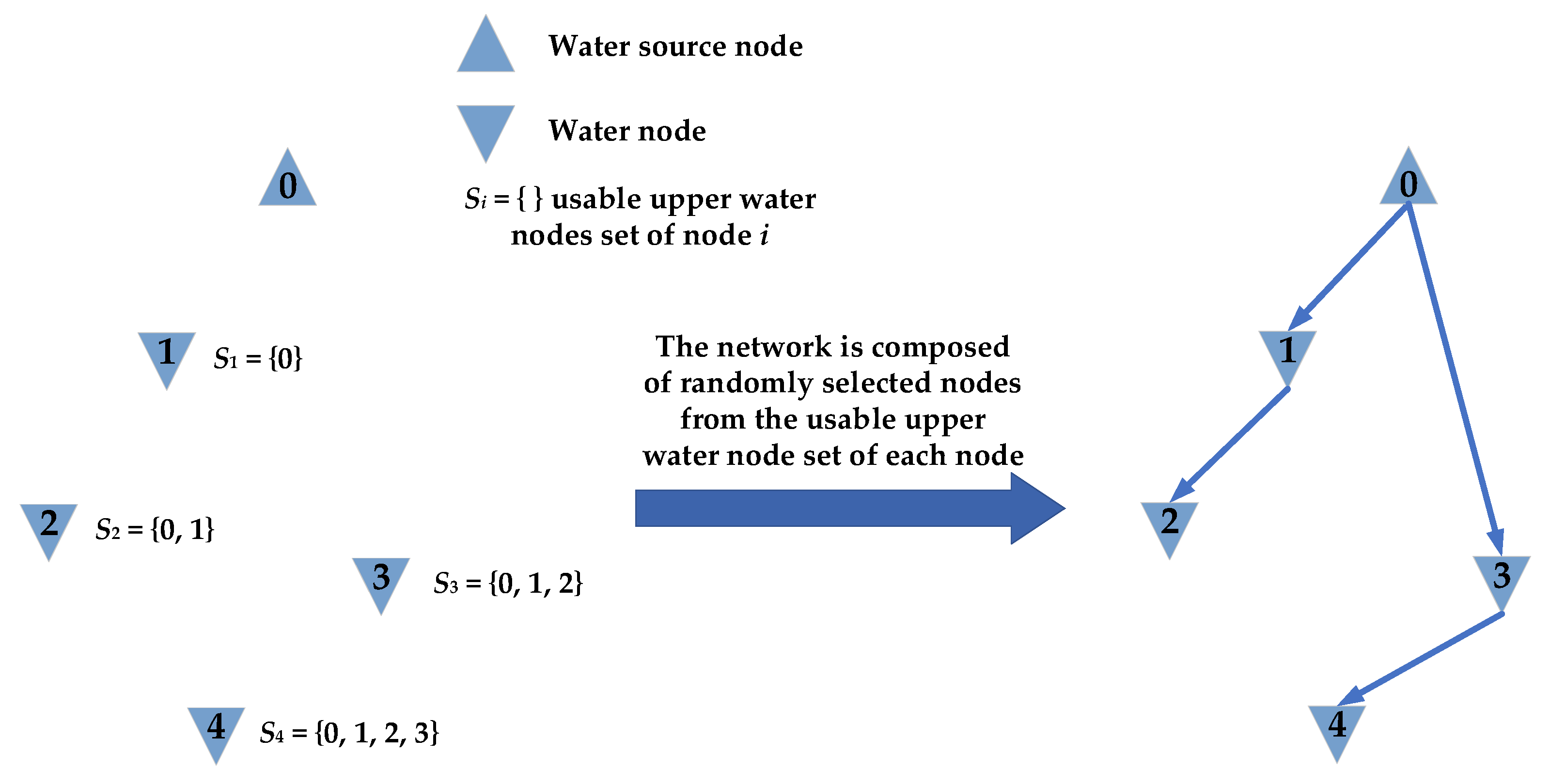
For the pipe network planning problem, current solutions require a preliminary connection diagram of the pipe network corresponding to the actual working conditions of the project and the experience of the design personnel to ensure the single-point water supply principle of a tree-type pipe network [3]. This study introduced the concept of an upper water node into the traditional pipe network planning model and transformed the pipe network deployment planning problem into the selection and combination of water-consuming nodes and their corresponding upper water nodes; this ensured the single-point water supply principle of the tree-type pipe network. Compared to the traditional pipe network deployment method, the improved pipe network planning model does not require the use of a preliminary connection diagram of the pipe network, thereby improving the versatility of the model. The improved pipe network planning model is described below.

The parameters of the water source point N₀ of the irrigation pipe network are denoted as (x₀, y₀, E_w), and the parameters of the water-consuming node N_i are denoted as (x_i, y_i, G_i) (i = 1, 2, …, N), where x_i and y_i indicate the ground coordinates of the node and G_i indicates the ground elevation of the node. For any water-consuming node N_i, its usable set of upper water nodes S_i is shown in Equation (5).

$$\begin{array}{c}{S}_i=\end{array}\left\{N_0,N_h|G_h\ge G_i\right\}\begin{array}{c}\end{array}\left(h=1,2,\dots ,N,h\ne i\right)$$

(5)

Then, for node N_i, there must exist one upper water node N_h ϵ S_i such that the pipe i connecting these two nodes have a length of L_ih, which can be obtained via Equation (6).

$$\begin{array}{c}{L}_{ih}=\end{array}\sqrt{{\left(x_i-x_h\right)}^2+{\left(y_i-y_h\right)}^2+{\left(G_i-G_h\right)}^2}$$

(6)

Denoting the diameter of pipe i as D_ih, the investment cost of the pipe network can be calculated using Equation (7).

$$\begin{array}{c}\min \begin{array}{c}Ic\end{array}=\end{array}{\displaystyle \sum _{i=1}^{N}f\left(D_{ih},L_{ih}\right)}={\displaystyle \sum _{i=1}^N\left(\alpha +\beta \times D_{ih}^{\gamma }\right)\times L_{ih}}$$

(7)

According to the single-point water supply principle of a tree-type irrigation pipe network, to ensure the connectivity of the pipe network, there is one and only one connection pipe i connected to any water-consuming node N_i (i = 1, 2, …, N) that supplies water to this node. In a self-pressure tree-type irrigation pipe network, the node connected to the other end of pipe i is specified as N_h (h ≠ i), where the node N_h is the upper water node of the node N_i, meaning that water flows through pipe i from node N_h to node N_i. This study introduced the upper water node concept to the improved pipe network planning model to ensure the water supply connectivity of the pipe network deployment. To further improve the robustness of the pipe network, the ground elevation G_i of the node N_i should not be lower than the ground elevation G_h of the node N_h. A schematic diagram of the calculation process for each upper water node of the improved pipe network planning model is shown in Figure 1. Note that, if there are multiple water-consuming nodes with the same ground elevation in the pipe network, then the average distance between each water-consuming node and its set of upper water nodes is calculated separately. The water-consuming node with the smallest average distance has priority over the other nodes and becomes the upper water node of the other water-consuming nodes.

3. The CSO and ICSO-ASV Algorithms

3.1. Traditional CSO Algorithm

The CSO algorithm simulates the hierarchy of a chicken swarm and the food-searching behavior of different individuals [14]. A chicken swarm consists of several groups, each of which is composed of one rooster, several hens, and several chicks. According to the functional fitness value of the problem-solving function, the chicken swarm is divided into three swarms: the rooster swarm, the hen swarm, and the chick swarm. From all the individuals, the set of individuals with the best fitness values is selected to be the rooster swarm, the set of individuals with the worst fitness values is selected to be the chick swarm, and the remainder of the individuals composes the hen swarm. The mother–child relationship between the chicks and hens is established randomly. The hierarchy, dominance, and mother–child relationships are updated at every generation.

The number of individuals in the chicken swarm is denoted as N. RN, HN, CN, and MN denote the numbers of roosters, hens, chicks, and mothers of chicks, respectively. In each group, the position of the rooster is updated, as shown in Equations (8) and (9).

$$x_{i,j}^{t+1}=x_{i,j}^t\times \left(1+Randn(0,{\sigma }^2)\right)$$

(8)

$${\sigma }^2=\{\begin{array}{cc}1,& f_i\le f_k\\ \exp \left(\frac{\left(f_k-f_i\right)}{\left|f_i\right|+\epsilon }\right),& f_i>f_k,\end{array}k\in \left[1,N\right],k\ne i.$$

(9)

Here, Randn(0, σ²) represents a random number generated using a Gaussian distribution with a mean of zero and a standard deviation of σ², t indicates the current number of iterations, ε is the smallest constant used to avoid zero-division errors, k is the index of a rooster randomly selected from another group, and f_i is the fitness value of the rooster i.

The hens follow the rooster in their group to search for food, and their positions are updated as shown in Equations (10)–(12).

$$\begin{array}{c}{x}_{i,j}^{t+1}=x_{i,j}^t+S_1\times Rand\times \left(x_{r_1,j}^t-x_{i,j}^t\right)+\\ S_2\times Rand\times \left(x_{r_2,j}^t-x_{i,j}^t\right)\end{array}$$

(10)

$$S_1=\exp \left(\left(f_i-f_{r_1}\right)/\left(abs\left(f_i\right)+\epsilon \right)\right)$$

(11)

$$S_2=\exp \left(f_{r_2}-f_i\right)$$

(12)

Here, Rand represents a uniform random number within the range of [0,1], r₁ is the index of the rooster in the same group as hen i, r₂ is the index of a randomly selected rooster or hen superior to hen i, and r₁ ≠ r₂.

Chicks follow their mothers in their group to search for food, and their positions are updated as shown in Equation (13).

$$x_{i,j}^{t+1}=x_{i,j}^t+FL\times \left(x_{m,j}^t-x_{i,j}^t\right)$$

(13)

Here, x^t_m,j indicates the position of the mother of chick i and FL ϵ [0,2], which represents the foraging and following coefficient of a chick following its mother.

3.2. ICSO-ASV Algorithm

3.2.1. Improved Control Coefficient Pair of the Hen Swarm

In the traditional CSO algorithm, the process of updating the position of a hen is primarily affected by factors such as the rooster in the hen’s group, another randomly selected rooster or hen, and the control coefficients S₁ and S₂ of the two previously mentioned individuals, as shown in Equation (10). In Equation (10), S₁ and S₂ represent the degree of closeness of the corresponding hen individual to the rooster individual in that hen’s group and the degree of competition with other individuals, respectively. In each iteration, the values of S₁ and S₂ are directly related to the fitness values of the rooster individual in the hen’s group and the other randomly selected individual, without including a comprehensive consideration of the impact of the current overall status of the swarm on the hen individual, as shown in Equations (11) and (12). However, the calculation processes of S₁ and S₂ are independent of each other, making it difficult to directly coordinate the impact of the rooster in the hen’s group and the other individual on the hen. Based on the above analysis, this study proposed an improved control coefficient pair C₁ and C₂ for the hen swarm, as shown in Equations (14) and (15).

$$C_1=\alpha \left(1-\exp \left(-|F_{avg}-F_{\mathit{best}}|\right)\right)+\beta (1-b)$$

(14)

$$C_2=R-C_1$$

(15)

Here, F_avg is the current average functional fitness value of the chicken swarm; F_best is the functional fitness value of the current optimal chicken swarm individual; |F_avg − F_best| is the difference between the average value of the population fitness value and the optimal individual value, indicating the proximity of individuals in the population to the optimal individual; b = t/T_max is the proportion coefficient of the algorithm iteration process, where T_max is the maximum number of iterations of the algorithm and b ϵ (0, 1); and the coefficient C₁ is primarily affected by the fitness value of the objective function and the iterative process of the algorithm. In the equations, the weight coefficients are the constants α and β, where α,β ϵ [1,1.5]. We denote the sum of C₁ and C₂ as the constant R; accordingly, C₂ = R − C₁.

As the iterative process of the algorithm changes, the value of the coefficient C₁ gradually decreases from α + β to zero and the value of the coefficient C₂ gradually increases from R − (α + β) to R. Considering that C₁ and C₂ characterize the impact of the rooster in the hen’s group and the competing individual on the hen individual, respectively, in the early stage of the algorithm’s execution, the difference between the average value of the chicken swarm and the optimal individual is relatively large and a larger C₁ can increase the proportion of learning of the hen individual from the rooster in the hen’s group and reduce the competition with other individuals; accordingly, the hen individual can quickly approach the rooster individual in its group in terms of its fitness value, thereby accelerating the convergence rate of the algorithm. In the later stage of the algorithm’s execution, the difference between the average value of the chicken swarm and the optimal individual is relatively small and a larger C₂ can increase the degree of competition between the hen individual and other individuals and reduce the proportion of learning from the rooster individual in the hen’s group; this allows the hen swarm to maintain good population diversity and avoids the premature convergence of the algorithm. Therefore, the improved control coefficient pair proposed in this study can adapt to the changes in the iterative process of the algorithm because it fully takes into consideration the impact of the current overall state of the chicken swarm on the hen individual and adaptively adjusts the impact of the rooster in the hen’s group and other individuals on the hen individual via mutually restrained cooperation.

3.2.2. Adaptive Mutation Factors

In this paper, the adaptive mutation factors V₁ and V₂ are introduced into the position update process for the rooster and chick swarms, as shown in Equation (16).

$$V_1=\frac{C_2}{\gamma },V_2=\frac{C_1}{\gamma }$$

(16)

Here, C₁ and C₂ are the improved control coefficient pair and γ is a constant used to ensure that the value ranges of V₁ and V₂ do not exceed 1. Because C₁ and C₂ can change adaptively according to the functional fitness value and the algorithm iteration process, the mutation factors V₁ and V₂ can also change adaptively to dynamically adjust the search operations of the rooster and chick swarms as the algorithm optimization process progresses.

After the position update of a rooster individual is completed, a random number β₁ ϵ [0,1] is generated. If β₁ < V₁ and f_i > P_i are satisfied, the rooster individual performs an adaptive mutation operation, as shown in Equation (17). After the position update of a chick individual is completed, a random number β₂ ϵ [0,1] is generated. If β₂ < V₂ is satisfied, then the chick individual is randomly reset.

$$x_{i,j}^{t+1}=x_{i,j}^t+F\times \left(x_{max}-x_{min}\right)$$

(17)

Here, P_i represents the optimal value of the rooster individual i, x_max − x_min represents the boundary distance of the feasible solution domain of the function, and F is the coefficient of mutation such that the rooster individual uses the pre-mutation position as a center to randomly generate a new feasible solution within a small range.

In the early stage of the algorithm, the control coefficients satisfy C₁ > C₂ and the mutation factors satisfy V₂ > V₁, meaning that the probability of the rooster swarm performing a mutation operation is relatively small, while the probability of the chick swarm performing a mutation operation is relatively large; this is conducive to expanding the global search range of the chicken swarm to avoid falling into a local optimum in the early stage of the algorithm while maintaining the normal optimization of the rooster swarm. In the later stage of the algorithm, the control coefficients satisfy C₂ > C₁ and the mutation factors satisfy V₁ > V₂, suggesting that the probability of the rooster swarm performing a mutation operation is relatively large, while the probability of the chick swarm performing a mutation operation is relatively small; this is conducive to leading the chicken swarm to search around the optimal solution of the function, thereby improving the accuracy of the algorithm.

The population size of the ICSO-ASV algorithm is denoted as N, the number of roosters is denoted as RN, the number of chicks is denoted as CN, and the probability of the mutation operation for a rooster individual and a chick individual are denoted as V₁ and V₂, respectively. Therefore, the time complexity of the calculation of a single iteration is O(N + V₁ × RN + V₂ × CN), where 0 < V₁ < 1 and 0 < V₂ < 1. If the maximum number of iterations of the algorithm is denoted by T_max, then the time complexity of the ICSO-ASV algorithm is O([N + V₁ × RN + V₂ × CN] × T_max). The flow of the ICSO-ASV algorithm is described as follows.

Step 1:

Initialize the chicken swarm. Set the population size N, the number of roosters RN, the number of hens HN, the number of chicks CN, the number of chick mothers MN, the update period G, and the maximum number of iterations T_max. Calculate the fitness values of all the individuals in the chicken swarm, initialize the individual optimal value and the global optimal value, and set the number of iterations to t = 1.

Step 2:

Update C₁, C₂, V₁, and V₂ according to Equations (14)–(16).

Step 3:

If t % G = 1, reorder all the individuals in the flock according to their fitness values, establish the corresponding hierarchical order, and divide the subgroups.

Step 4:

Update the rooster individual according to Equations (8) and (9). If β₁ < V₁ and f_i > P_i are satisfied, then perform the adaptive mutation operation on the rooster individual according to Equation (17); update the hen individuals according to Equation (10); and update the chick individuals according to Equation (13). If β₂ < V₂ is satisfied, then randomly reset the chick individual.

Step 5:

Update and save the individual and global optimal values of the chicken swarm.

Step 6:

If the algorithm satisfies the iteration stop condition, then stop the iteration and output the optimal feasible solution; otherwise, go back to step 2.

3.3. ICSO-ASV Algorithm Performance Analysis

In this study, the performance of the ICSO-ASV algorithm was analyzed using 12 benchmark test functions, the results of which were then compared to those of the following six algorithms: PSO (Particle Swarm Optimization) [24], BA (Bat Algorithm) [25], CSO [14], ADLCSO [18], ICSO-a [19], and ICSO-b [20]. The 12 benchmark test functions are shown in

Table 1. Benchmark test functions.

Test Functions	Equation	Scope
Shifted sphere	$\begin{array}{c}{f}_1\left(x_i\right)=\end{array}{\displaystyle {\sum }_{i=1}^D{\left(x_i-10\right)}^2-450}$	[−100,100]
Shifted schwefel 1.2	$\begin{array}{c}{f}_2\left(x_i\right)=\end{array}{\displaystyle {\sum }_{i=1}^D{\left[{\displaystyle {\sum }_{j=1}^i\left(x_j-20\right)}\right]}^2}-450$	[−100,100]
Shifted rotated elliptic	$f_3\left(x_i\right)={\displaystyle {\sum }_{i=1}^D[{\left({10}^6\right)}^{\frac{t-1}{D-1}}{\left(x_i-i\right)}^2]}-450$	[−100,100]
Shifted rosenbrock	$\begin{array}{c}{f}_4\left(x_i\right)=\end{array}{\displaystyle {\sum }_{i=1}^{D-1}\left[100{\left(x_i^2-x_{i+1}\right)}^2+{\left(x_i-1\right)}^2\right]}+390$	[−100,100]
Griewank	$f_5\left(x_i\right)=({\displaystyle {\sum }_{i=1}^D{x}_i^2})/4000-{\displaystyle {\prod }_{i=1}^D\cos (x_i/\sqrt{i})}+1$	[−600,600]
Rastrigin	$f_6\left(x_i\right)=10D+{\displaystyle {\sum }_{i=1}^D[x_i^2-10\cos \left(2\pi x_i\right)]}$	[−5.12,5.12]
Ackley N.4	$f_7\left(x_i\right)={\displaystyle {\sum }_{i=1}^{D-1}[\exp (-0.2)\sqrt{x_i^2+x_{i+1}^2}+3\left(\cos \left(2x_i\right)+\sin \left(2x_{i+1}\right)\right)]}$	[−35,35]
Periodic	$f_8\left(x_i\right)=1+{\displaystyle {\sum }_{i=1}^D{\sin }^2(x_i)}-0.1\exp (-{\displaystyle {\sum }_{i=1}^D{x}_i^2})$	[−10,10]
Schwefel 2.13	$\begin{array}{l}{f}_9\left(x_i\right)={\displaystyle \sum _{i=1}^D{\left[{\displaystyle \sum _{j=1}^D\left(a_{ij}\sin {\alpha }_j+b_{ij}\cos {\alpha }_j\right)}-{\displaystyle \sum _{j=1}^D\left(a_{ij}\sin x_j+b_{ij}\cos x_j\right)}\right]}^2}-460\\ a_{ij}=\mathrm{rand}(-100,100),b_{ij}=\mathrm{rand}(-100,100),{\alpha }_j=\mathrm{rand}(-\pi ,\pi )\end{array}$	[−π,π]
Levy	$\begin{array}{l}{f}_{10}\left(x_i\right)={\sin }^2\left(\pi y_1\right)+{\displaystyle \sum _{i=1}^{D-1}{\left(y_i-1\right)}^2}\left[1+10{\sin }^2\left(\pi y_i+1\right)\right]+\\ {\left(y_D-1\right)}^2\left[1+{\sin }^2\left(2\pi y_D\right)\right]y_i=1+\left(x_i-1\right)/4\end{array}$	[−10,10]
Generalized Penalized N.1	$\begin{array}{l}\begin{array}{c}{f}_{11}\left(x_i\right)=\end{array}\left\{10{\sin }^2\left(\pi y_1\right)+{\displaystyle {\sum }_{i=1}^{D-1}{\left(y_i-1\right)}^2\left[1+10{\sin }^2\left(\pi y_{i+1}\right)\right]+{\left(y_D-1\right)}^2}\right\}\times \\ \pi /D+{\displaystyle {\sum }_{i=1}^{D}u\left(x_i,10,100,4\right)}{y}_i=1+\left(x_i+1\right)/4\end{array}$	[−50,50]
Generalized Penalized N.2	$\begin{array}{l}\begin{array}{c}{f}_{12}\left(x_i\right)=\end{array}\left\{{\sin }^2\left(3\pi x_1\right)+{\displaystyle {\sum }_{i=1}^{D-1}{\left(x_i-1\right)}^2\left[1+{\sin }^2\left(3\pi x_{i+1}\right)\right]+{\left(x_D-1\right)}^2}\right\}\times \\ 0.1+{\displaystyle {\sum }_{i=1}^{D}u\left(x_i,5,100,4\right)}\end{array}$	[−50,50]

. The benchmark test functions f₁–f₃ are single-peak functions, while functions f₄–f₁₂ are multi-peak functions; the functions f₁–f₄ are shifted functions with minimum values depending on the shifted data in the equation; and functions f₅, f₆, and f₉–f₁₂ have a minimum value of 0, whereas the minimum value of f₇ is approximately −150 and the minimum value of f₈ is 0.9.

The algorithm test environment consisted of a Microsoft Windows 10 64-bit, Intel^® Core™ i5-7300HQ CPU @ 2.50 GHz and 8.0 GB RAM with MATLAB R2018a (source info: MathWorks, Natick, MA, USA). The parameter settings of each control algorithm are shown in

Table 2. Algorithm parameter settings.

Algorithm	Parameter Settings
PSO 1	Learning factor c1 = c2 = 2; inertia weight w = 0.4
BA 2	Pulse frequency Fmax = 0, Fmin = −2; the initial range of the pulse loudness A was (1,2); the initial range of the pulse emission frequency R was (0,0.5), Rmax = 0.9
CSO 3	RN = 0.15N, HN = 0.7N, CN = 0.15N, MN = 0.5HN, G = 10, FL ϵ [0.5,0.9]
ICSO-ASV 4	R = 3, α = 1, β = 1.5, γ = 3.5; the other parameters were kept consistent with the traditional CSO algorithm
ADLCSO 5	K = 20, a = 5; the other parameters were kept consistent with the traditional CSO algorithm
ICSO-a 6	A0 = 1, R0 = 0.9; the other parameters were kept consistent with the traditional CSO algorithm
ICSO-b 7	wmax = 0.9, wmin = 0.4; the other parameters were kept consistent with the traditional CSO algorithm

¹ Particle Swarm Optimization; ² Bat Algorithm; ³ Chicken Swarm Optimization; ⁴ Improved Chicken Swarm Optimization using Adaptive Search and Variation; ⁵ Adaptive Dynamic Learning Chicken Swarm Optimization; ⁶ Improved Chicken Swarm Optimization (Sun et al. [19]); ⁷ Improved Chicken Swarm Optimization (Fu et al. [20]).

. The population size of all algorithms was set to 100, the number of independent executions was 50, the maximum number of iterations was 500, and all other general parameters were kept consistent.

A comparative analysis was conducted for the ICSO-ASV algorithm, three standard algorithms (PSO, BA, and CSO), and three ICSOAs (ADLCSO, ICSO-a, and ICSO-b) based on the 30D and 50D benchmark test functions. The results of each algorithm based on the 30D benchmark test functions are shown in

Table 3. Solution results for the 30D benchmark test functions.

Function		PSO	BA	CSO	ADLCSO	ICSO-a	ICSO-b	ICSO-ASV
f1	best	−4.4198 × 102	−4.3082 × 102	−3.8003 × 102	−4.4603 × 102	1.1612 × 102	3.1889 × 103	−4.5000 × 102
	worst	5.3485 × 103	−3.3984 × 102	9.4911 × 102	1.1412 × 103	9.7823 × 102	4.6067 × 103	−4.5000 × 102
	mean	−9.5422 × 101	−3.9981 × 102	6.6306 × 101	−2.8940 × 102	6.1614 × 102	3.9134 × 103	−4.5000 × 102
	std	1.2912 × 103	2.3069 × 101	2.6787 × 102	3.0979 × 102	1.8367 × 102	3.7222 × 102	5.6809 × 10−4
f2	best	1.7770 × 104	1.7820 × 104	2.4538 × 104	1.7531 ×104	2.1433 × 104	8.5751 × 104	1.7530 × 104
	worst	2.4743 × 105	1.9323 × 104	6.6164 × 104	4.6608 × 104	2.8007 × 104	1.4533 × 105	1.7530 × 104
	mean	3.0376 × 104	1.8266 × 104	4.3612 × 104	2.0052 × 104	2.4034 × 104	1.2456 × 105	1.7530 × 104
	std	3.5114 × 104	3.0574 × 102	9.5788 × 103	4.7357 × 103	1.5189 × 103	1.3283 × 104	7.0028 × 10−3
f3	best	8.9319 × 105	4.6584 × 105	1.0036 × 106	8.3129 × 105	2.3226 × 106	6.3700 × 107	−4.4971 × 102
	worst	6.7774 × 107	1.5778 × 107	6.0109 × 107	3.3745 × 107	2.0906 × 107	2.1914 × 108	−4.4535 × 102
	mean	1.5552 × 107	3.5486 × 106	9.2439 × 106	7.0264 × 106	9.6165 × 106	1.3499 × 108	−4.4834 × 102
	std	1.9172 × 107	3.4124 × 106	8.6587 × 106	6.7121 × 106	4.0486 × 106	3.7299 × 107	1.1339
f4	best	2.6352 × 103	7.9102 × 103	4.3791 × 106	6.8771 × 102	8.9495 × 105	6.0103 × 107	4.8889 × 102
	worst	1.6422 × 106	2.8984 × 105	6.5733 × 107	6.6123 × 107	9.7748 × 106	1.4435 × 108	1.2563 × 103
	mean	1.9988 × 105	9.2552 × 104	1.9298 × 107	2.3041 × 106	4.6969 × 106	1.0252 × 108	6.1318 × 102
	std	4.3595 × 105	6.9864 × 104	1.3209 × 107	1.0592 × 107	2.1167 × 106	2.0457 × 107	1.7386 × 102
f5	best	0	1.4943 × 10−1	0	0	0	0	0
	worst	1.0648	1.0419	1.0284 × 10−1	2.8137 × 10−2	0	0	4.4409 × 10−16
	mean	2.3734 × 10−1	8.6525 × 10−1	2.0570 × 10−3	2.5520 × 10−3	0	0	8.8818 × 10−18
	std	3.6956 × 10−1	1.7333 × 10−1	1.4544 × 10−2	6.6883 × 10−3	0	0	6.2804 × 10−17
f6	best	0	1.6315 × 10−2	0	0	0	0	0
	worst	9.1447 × 101	1.0708 × 102	0	1.0870 × 102	0	0	0
	mean	2.8520 × 101	2.3136 × 101	0	1.2744 × 101	0	0	0
	std	2.6732 × 101	2.4829 × 101	0	2.2205 × 101	0	0	0
f7	best	−7.2522 × 101	−8.5097 × 101	−7.3559 × 101	−7.4302 × 101	−8.1469 × 101	−1.1934 × 101	−8.5308 × 101
	worst	7.5589 × 101	−3.1056 × 101	−4.8019 × 101	−4.3127 × 101	−2.6206 × 101	9.7808	−7.1335 × 101
	mean	−3.6711 × 101	−7.1083 × 101	−6.5206 × 101	−6.3945 × 101	−6.8844 × 101	1.1971	−7.9057 × 101
	std	3.0670 × 101	1.5813 × 101	5.1834	7.0511	1.3605 × 101	5.2720	3.2252
f8	best	9.0002 × 10−1	1.0044	9.0000 × 10−1	1.0384	9.0000 × 10−1	9.0000 × 10−1	9.0000 × 10−1
	worst	3.7276	3.2981	1.8424	7.5581	9.2725 × 10−1	2.0576	9.0104 × 10−1
	mean	2.0006	1.8181	1.0942	3.3441	9.0104 × 10−1	1.2782	9.0002 × 10−1
	std	8.0633 × 10−1	5.7238 × 10−1	2.6566 × 10−1	1.7095	3.8629 × 10−3	2.9270 × 10−1	1.4686 × 10−4
f9	best	1.0917 × 105	1.4679 × 105	7.7440 × 104	4.5150 × 104	4.0807 × 105	6.5180 × 105	4.6151 × 103
	worst	9.2474 × 105	1.7595 × 106	4.8612 × 105	3.8448 × 105	1.5760 × 106	1.2887 × 106	1.2667 × 105
	mean	4.2627 × 105	6.5295 × 105	2.5861 × 105	1.9235 × 105	8.6552 × 105	1.0290 × 106	3.9165 × 104
	std	1.9413 × 105	3.8037 × 105	8.0373 × 104	6.7142 × 104	2.2966 × 105	1.4234 × 105	2.7675 × 104
f10	best	3.1835 × 10−1	6.2016 × 10−6	6.5353 × 10−1	6.3698 × 10−1	1.1833 × 10−1	1.6612	3.0642 × 10−6
	worst	1.3363 × 101	1.2156 × 10−1	1.7498	1.9599 × 101	7.0435 × 10−1	2.4077	5.8098 × 10−5
	mean	2.2097	4.9715 × 10−3	1.1404	2.5014	2.5876 × 10−1	2.0564	1.6873 × 10−5
	std	2.8557	1.7282 × 10−2	2.6750 × 10−1	4.5769	1.0182 × 10−1	1.4906 × 10−1	1.1682 × 10−5
f11	best	4.9022 × 10−3	1.3304 × 10−5	3.4243 × 10−2	2.7791 × 10−2	4.8095 × 10−3	1.5586 × 10−1	3.4846 × 10−7
	worst	2.7097	2.5880 × 10−1	1.0322	3.2997 × 101	1.3432 × 10−1	4.8938 × 10−1	7.5615 × 10−6
	mean	2.4630 × 10−1	1.6127 × 10−2	1.7266 × 10−1	6.7224	1.5590 × 10−2	3.3875 × 10−1	1.5938 × 10−6
	std	5.3089 × 10−1	3.8480 × 10−2	1.7404 × 10−1	7.9878	1.7781 × 10−2	7.6893 × 10−2	1.4602 × 10−6
f12	best	3.6434 × 10−1	2.7695 × 10−4	5.7850 × 10−1	4.4193 × 10−1	2.1136 × 10−2	2.0960	7.2050 × 10−7
	worst	6.1921	8.7633 × 10−1	2.4046	4.6132 × 101	2.9589 × 10−1	2.7165	1.1992 × 10−4
	mean	2.1014	7.4953 × 10−2	1.1036	2.6501	1.2770 × 10−1	2.5493	1.8130 × 10−5
	std	1.2645	1.5000 × 10−1	2.9481 × 10−1	8.7195	5.1404 × 10−2	1.2976 × 10−1	2.0787 × 10−5

.

Table 3 indicates that, of the three standard algorithms, the BA algorithm had certain advantages in solving some of the test functions, whereas the CSO algorithm could find the global optimal value of the function f₆. Both of these algorithms were superior to the PSO algorithm; however, the results of the three standard algorithms for most of the test functions were within the same or similar order of magnitude. Of the three ICSOAs, the ADLCSO algorithm obtained the best single-peak function solution results and the ICSO-a algorithm obtained the best multi-peak function solution results. Overall, these two algorithms performed better than the ICSO-b algorithm.

Table 3 indicates that the results of the ICSO-ASV algorithm were better than those of the control algorithms overall. For the shifted functions f₁ and f₃ and the multi-peak functions f₆–f₈ and f₁₀–f₁₂, the ICSO-ASV algorithm could not only find the global optimal value but also had a standard deviation close to 0, indicating that it had a better solution accuracy and stability than the control algorithms. For the function f₅, the average value generated by the ICSO-ASV algorithm was slightly worse than those generated by the ICSO-a and ICSO-b algorithms, but the global optimal value could still be found. For the other benchmark functions, the solution results of the ICSO-ASV algorithm had obvious advantages. The accuracies of the solutions were improved by more than five orders of magnitude compared to those of the standard CSO algorithm for half of the test functions, especially for functions f₃, f₁₁, and f₁₂, and the solution accuracy of the ICSO-ASV algorithm was higher than that of the optimal control algorithm by more than three orders of magnitude.

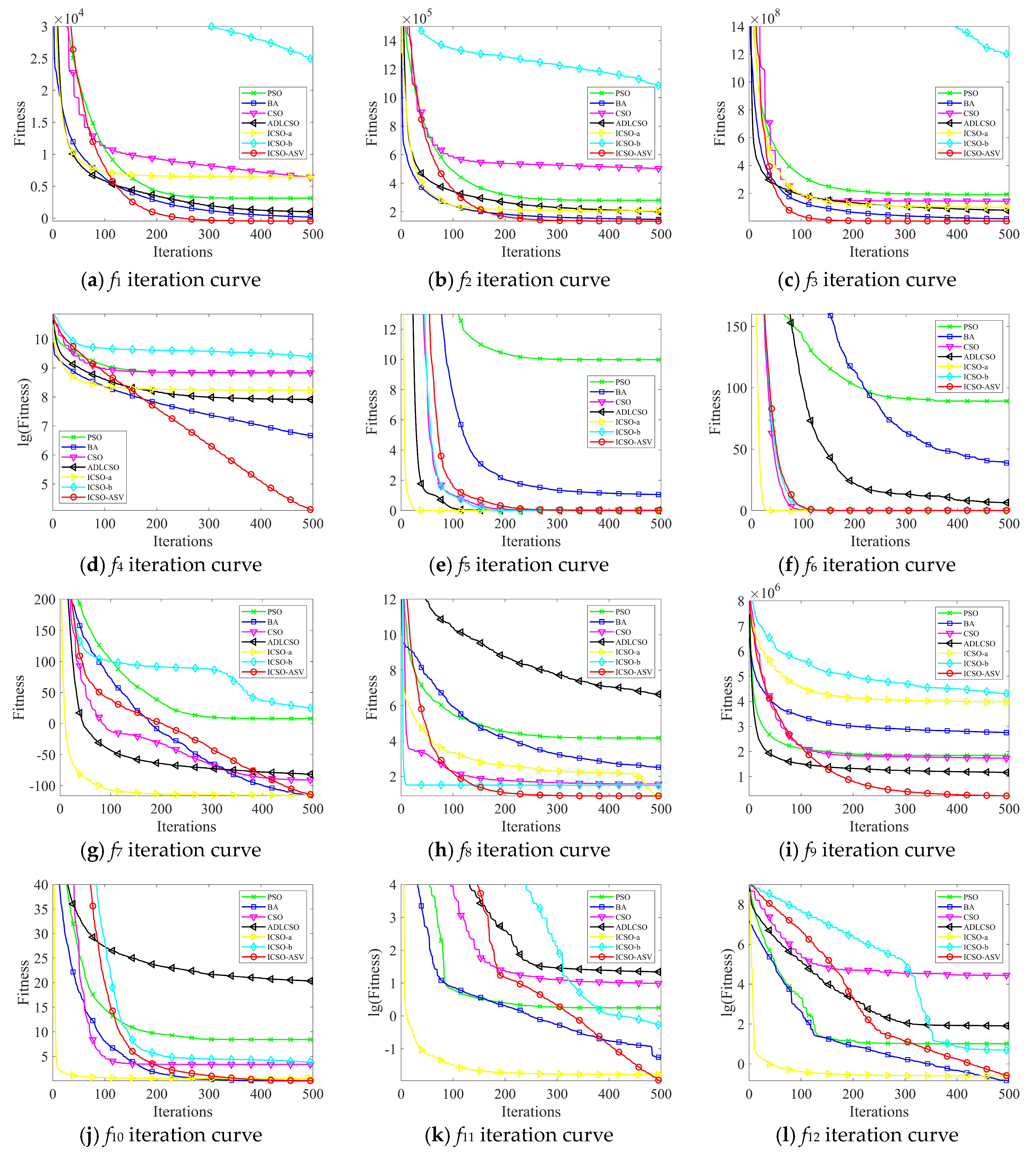
The iterative curves of the mean fitness values of each algorithm based on the 50D test functions are shown in Figure 2, where some results are logarithmic. Figure 2 indicates that, of the three standard algorithms, the CSO algorithm had certain advantages in terms of the convergence speed, but the BA algorithm could obtain better optimization results for multiple functions. When comparing the CSO algorithm to the ICSOAs, the ICSO-a algorithm had certain advantages in terms of the convergence speed and could obtain better optimization results for multiple functions. The ICSO-ASV algorithm had relatively obvious advantages in terms of the solution accuracy and avoiding local optima in comparison to the control algorithms. The optimization curves of the functions f₄, f₇, f₁₁, and f₁₂ show that, as the number of iterations increases, the ICSO-ASV algorithm did not fall into a local optimum and its solution accuracy could be further improved.

4. Design of an Irrigation Pipe Network Based on the ICSO-ASV Algorithm

4.1. Analysis of the Improved Pipe Network Planning Model

The decision variables of the improved pipe network planning model include the length L_ih and the diameter D_ih of the connecting pipe between the water-consuming node N_i (i = 1, 2, …, N) and its upper water node N_h (h = 1, 2, …, N, h ≠ i), meaning that the solution space of the planning model is {L_ih, D_ih}. If there are N water-consuming nodes in the pipe network, then the dimension of the solution space is 2N. Considering that the pipe length and the pipe diameter that meet market standards are both discrete variables, the solution space of the ICSO-ASV algorithm also needs to be discretized. Note that, for the water-consuming node N_i, there exists a continuous feasible solution {x_l, x_d} ϵ [0,1] in the solution space of the ICSO-ASV algorithm corresponding to the solution space of the planning model {L_ih, D_ih}. For the connection pipe length L_ih, the upper water node N_h needs to be selected from the set of upper water nodes S_i belonging to the water-consuming node N_i; the corresponding relationship between x_l and N_h indexed as T_L in the set S_i is shown in Equation (18). For the pipe diameter D_ih, the index of T_D in the pipe diameter set R can be determined according to Equation (18).

$$\{\begin{array}{ll}0\le x_l<{\displaystyle {\sum }_{m=1}^{T_L}1/\left|S_i\right|}\hfill & T_L=1\hfill \\ {\displaystyle {\sum }_{m=1}^{T_L-1}1/\left|S_i\right|}\le x_l<{\displaystyle {\sum }_{m=1}^{T_L}1/\left|S_i\right|}\hfill & T_L=2,3,\cdots ,\left|S_i\right|\hfill \\ 0\le x_d<{\displaystyle {\sum }_{m=1}^{T_D}1/\left|R\right|}\hfill & T_D=1\hfill \\ {\displaystyle {\sum }_{m=1}^{T_D-1}1/\left|R\right|}\le x_d<{\displaystyle {\sum }_{m=1}^{T_D}1/\left|R\right|}\hfill & T_D=2,3,\cdots ,\left|R\right|\hfill \end{array}$$

(18)

Here, |S_i| represents the number of elements in the set S_i and |R| represents the number of elements in the set R.

Because all water-consuming nodes in the pipe network need to meet the node pressure constraints, a penalty function is used to convert the pipe network planning model and the constraints into an unconstrained objective function, as shown in Equation (19).

$$\min F={\displaystyle \sum _{i=1}^N\left(\alpha +\beta \times D_{ih}^{\gamma }\right)\times L_{ih}+h\left(t\right)\times K}$$

(19)

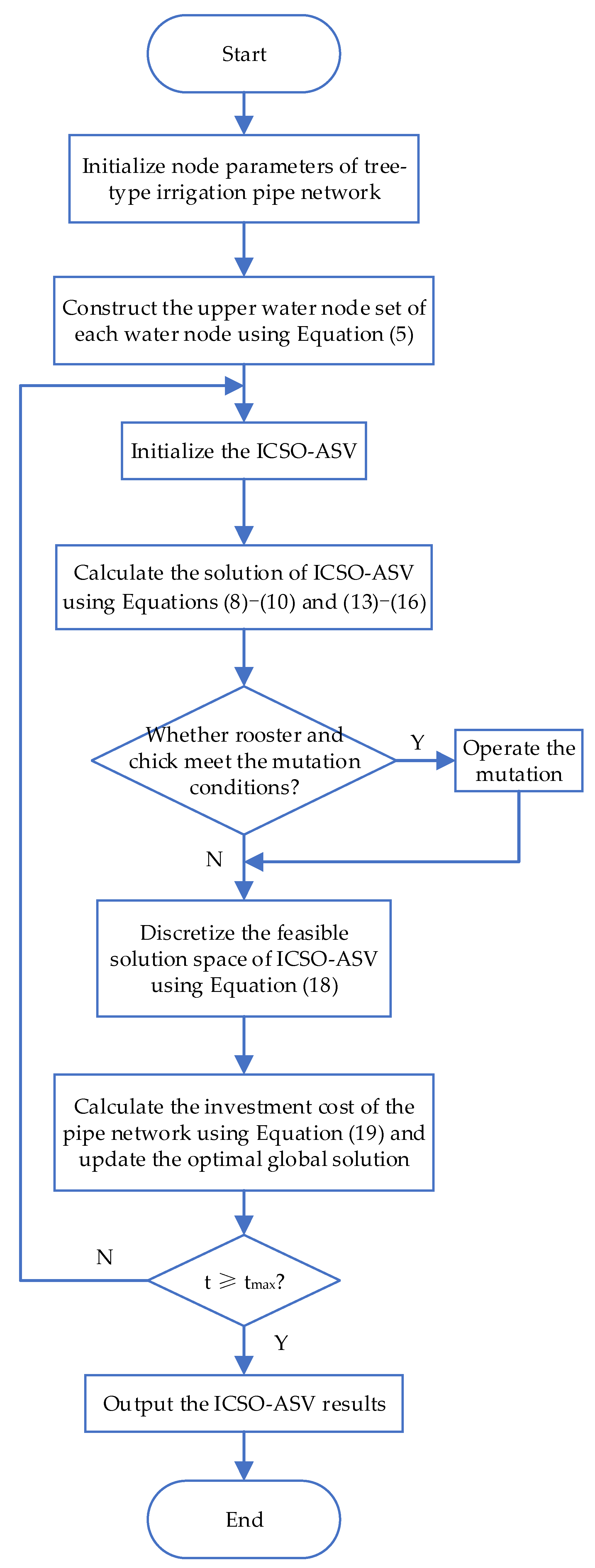
Here, h(t) = $\sqrt{t}$, where t indicates the current number of iterations, and K is the penalty function factor constructed according to the node pressure constraints, where the parameter settings are the same as those in Robinson and Rahmat-Samii [26]. A flow chart of a pipe network design based on the ICSO-ASV algorithm is shown in Figure 3.

4.2. Pipe Network Design Case I

This study used several algorithms, including GA (Genetic Algorithm) [27], BA [25], SABA (Self-Adaptive Bat Algorithm) [28], CSO [14], ADLCSO [18], ICSO-a [19], and ICSO-ASV to design pipe network cases. Pipe network design case I included one water source point and 14 water-consuming nodes. Note that the improved pipe network planning model proposed in this paper can ensure the water supply connectivity of the pipe network by selecting the upper water node of the water-consuming node and uses the node parameters to automatically calculate the lengths of all pipe connections; therefore, there is no need to use a preliminary connection diagram of the pipe network. The node parameters of the pipe network are shown in

Table 4. Pipe network parameters (15 nodes).

Sequence Number	Coordinate x (m)	Coordinate y (m)	Elevation Gi (m)	Water Flow Q (m3/h)	Sequence Number	Coordinate x (m)	Coordinate y (m)	Elevation Gi (m)	Water Flow Q (m3/h)
0	2085	1320	250	−295	8	2259	925	216	20
1	2681	377	220	20	9	1785	1098	216	20
2	2339	1652	220	20	10	1329	769	215	20
3	1121	1250	219	20	11	2018	421	214	20
4	1435	1359	219	25	12	562	2213	214	20
5	2071	1143	218	25	13	898	1212	212	20
6	2408	851	217	25	14	1314	2020	210	20
7	964	1637	216	20

, and the unit prices of the pipes are shown in

Table 5. Unit prices of pipes with different diameters.

Sequence Number	Pipe Diameter (mm)	Unit Price (Yuan)	Sequence Number	Pipe Diameter (mm)	Unit Price (Yuan)
0	50	2.5	5	140	8.6
1	75	3.6	6	160	11.0
2	90	4.5	7	180	13.0
3	110	6.2	8	200	15.6
4	125	7.0	9	225	19.2

. In the objective function, Equation (19), the pipe network cost parameters were calculated by fitting the data in Table 5, where the pipe network cost coefficients were α = 1.5 and β = 5.37 × 10⁻⁴ and the pipe network cost index was γ = 1.92 [3,9]. In the pressure-constrained equation, Equation (2), of the water-consuming nodes in the pipe network, the local head loss coefficient was ω = 1.1. Taking the rigid plastic pipe as the standard, the pipe head loss coefficients were θ = 9.48 × 10⁴, m = 1.77, and n = 4.77; the lowest water pressure of each node was P = 10 m; and in the pipe velocity constraint equation, Equation (3), V_max = 3 m/s and V_min = 0.5 m/s.

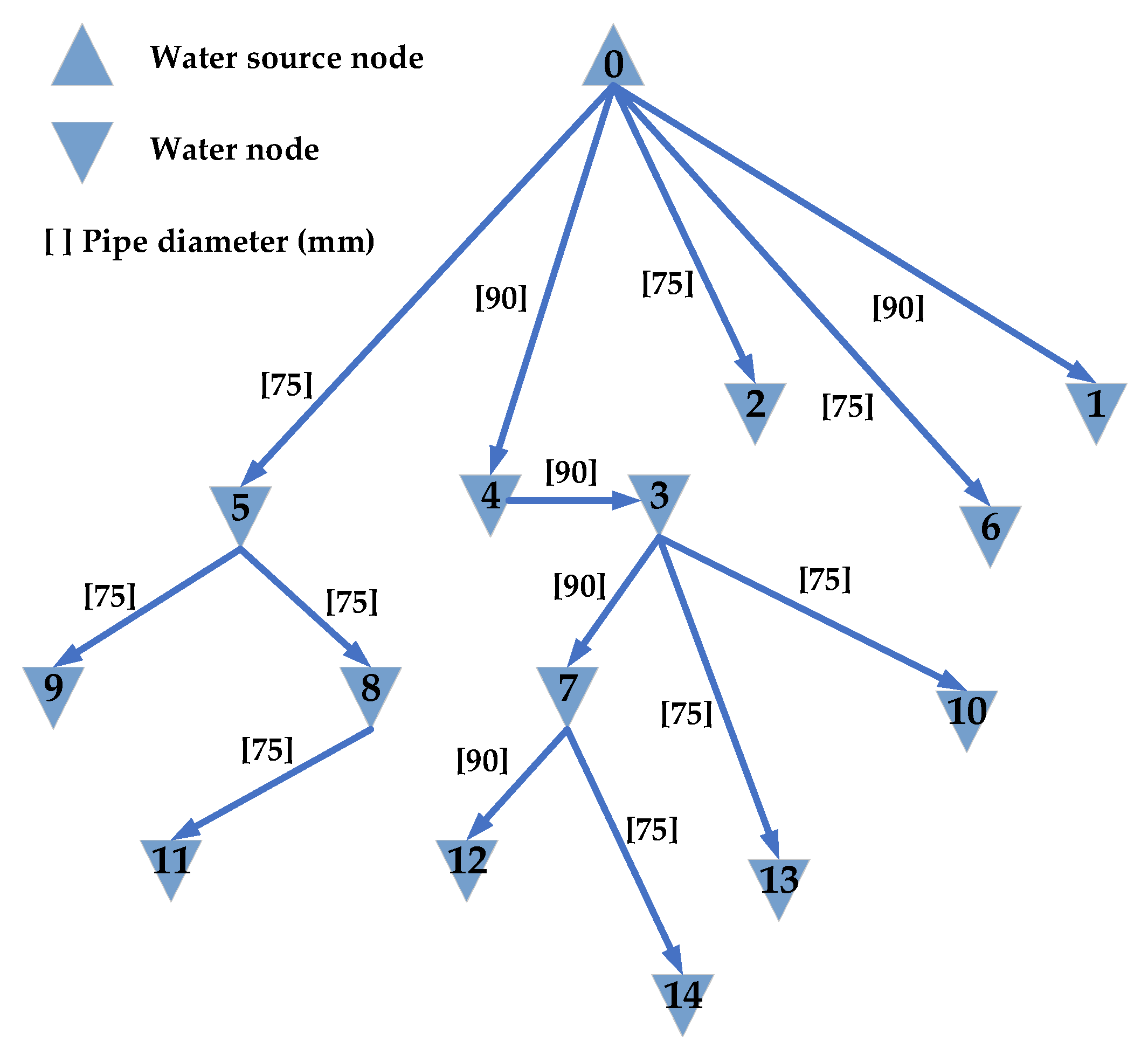
In this case, the population size of each algorithm was set to 40, the maximum number of iterations was 500, and the number of independent executions was 50. The design results of each algorithm based on the objective function, Equation (19), are shown in

Table 6. Design results of each algorithm (15 nodes).

Algorithms	Best (Yuan)	Mean (Yuan)	Worst (Yuan)
GA	31,114	36,734	46,053
BA	41,379	56,954	93,831
SABA	33,776	40,698	46,572
CSO	47,767	59,330	75,018
ADLCSO	30,109	38,227	50,528
ICSO-a	41,018	59,344	77,847
ICSO-ASV	27,611	32,338	41,937

, which details the optimal solution, mean value, and worst solution for the investment cost of the pipe network. The results show that, of the three standard algorithms, the design results based on the GA algorithm were superior overall compared to those of the traditional CSO algorithm in terms of the solution accuracy and stability, indicating that the traditional CSO algorithm was subject to falling into a local optimum when solving low-dimensional discrete combinatorial optimization problems. Compared to the traditional BA algorithm, the SABA algorithm showed a better performance. In terms of the optimal design results, all three ICSOAs obtained satisfactory design results. The design results based on the ICSO-ASV algorithm were superior overall compared to those of the other six algorithms in terms of the solution accuracy and stability. The ICSO-ASV algorithm yielded an optimal result of 27,611 yuan for the pipe network investment cost, and its mean design result was 42.20% lower than that of the traditional CSO algorithm. The design results indicate that the ICSO-ASV algorithm effectively reduced the probability of the algorithm falling into a local optimum, resulting in excellent algorithm performance. Therefore, the pipe network design method based on the ICSO-ASV algorithm proposed in this paper had relatively good accuracy.

The optimal design result of the pipe network based on the ICSO-ASV algorithm is shown in Figure 4.

4.3. Pipe Network Design Case II

With the expansion of the scale of the pipe network, that is, with an increase in the number of pipe network nodes, the solution space of the improved pipe network planning model increased exponentially and the difficulty of searching for the optimal solution of the model correspondingly increased. To further verify the scalability of the proposed design method, the second case investigated in this paper, pipe network design case II, included one water source point and 39 water-consuming nodes; the parameters of each node are shown in

Table 7. Pipe network parameters (40 nodes).

Sequence Number	Coordinate x (m)	Coordinate y (m)	Elevation Gi (m)	Water Flow Q (m3/h)	Sequence Number	Coordinate x (m)	Coordinate y (m)	Elevation Gi (m)	Water Flow Q (m3/h)
0	2085	1320	250	−930	20	2184	521	224	25
1	1810	1470	238	30	21	1904	816	223	25
2	2586	1510	237	30	22	575	734	223	20
3	1535	431	236	25	23	2420	1150	221	25
4	2210	1165	235	30	24	611	1335	221	25
5	1570	689	235	25	25	1363	1511	221	25
6	2681	1570	235	30	26	2681	377	220	20
7	1727	920	234	20	27	2339	1652	220	20
8	427	1765	234	25	28	1121	1250	219	20
9	1738	1526	233	30	29	1435	1359	219	25
10	1649	1389	232	30	30	2071	1143	218	25
11	1906	899	231	25	31	2408	851	217	25
12	373	1209	231	25	32	964	1637	216	20
13	976	1455	230	25	33	2259	925	216	20
14	1321	1169	228	25	34	1785	1098	216	20
15	1008	725	227	25	35	1329	769	215	20
16	2190	1031	227	20	36	2018	421	214	20
17	1230	1373	226	20	37	562	2213	214	20
18	870	1922	225	20	38	898	1212	212	20
19	1411	1703	225	30	39	1314	2020	210	20

.

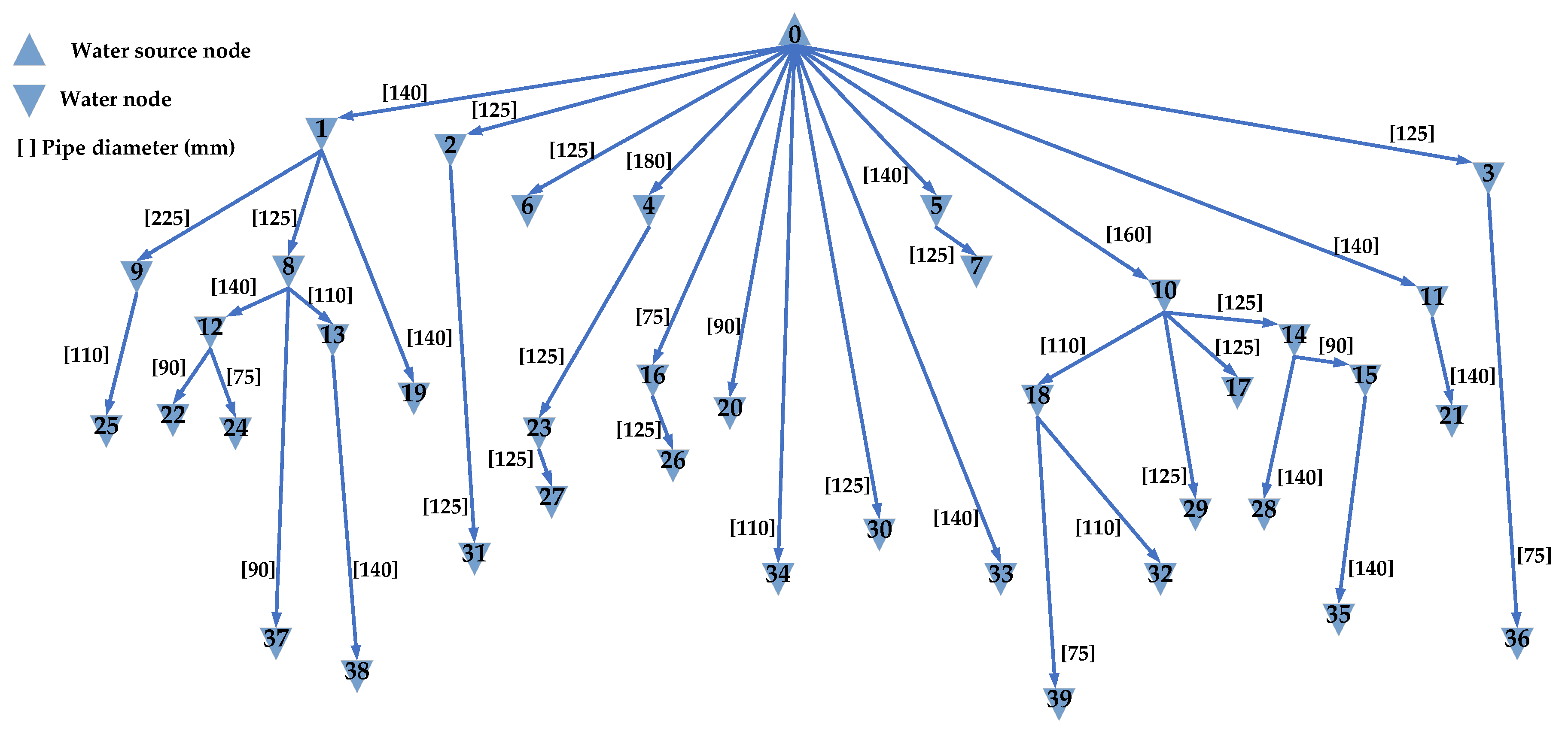
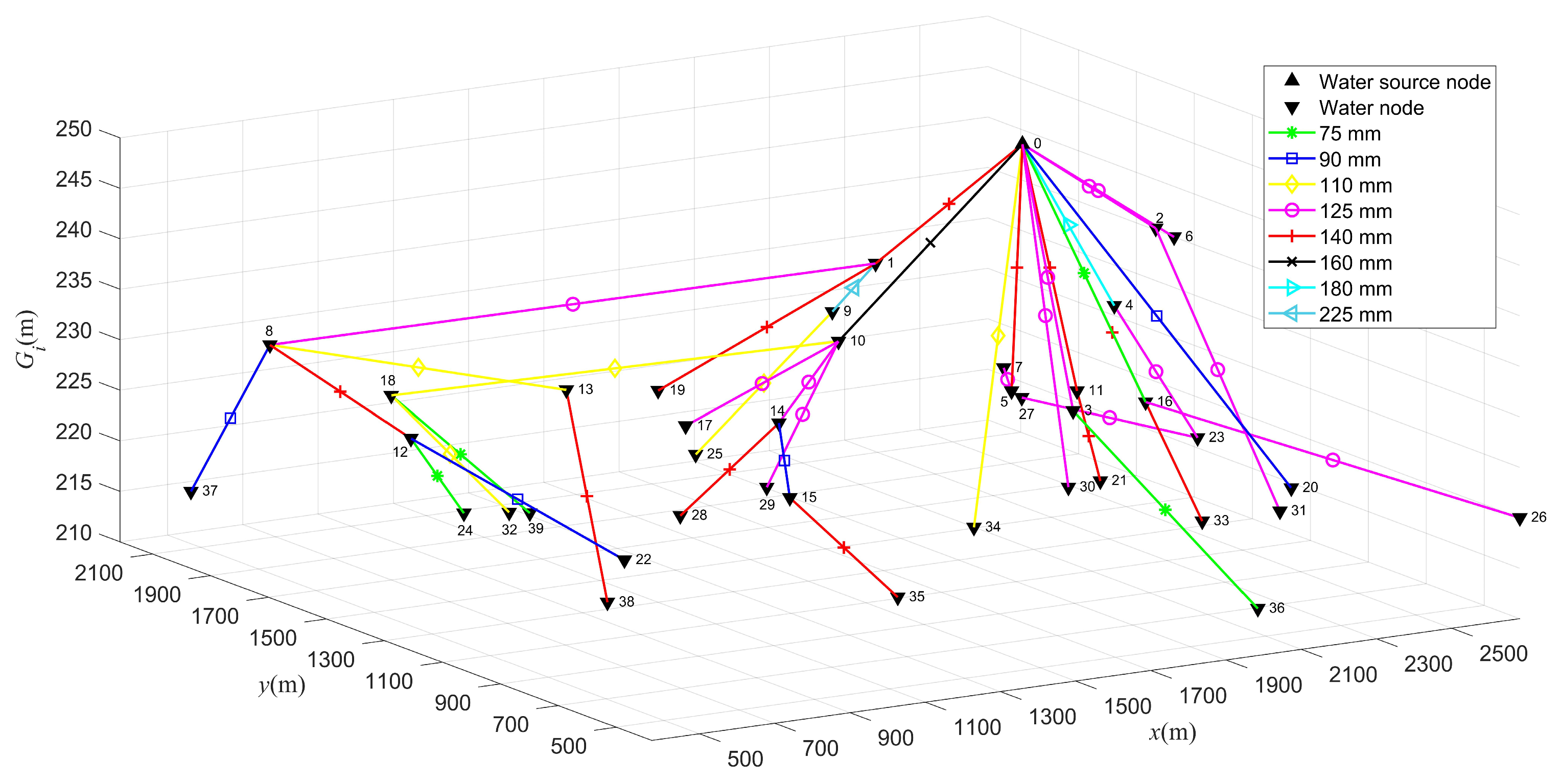
The results of the pipe network design based on each algorithm are shown in

Table 8. Design results of each algorithm (40 nodes).

Algorithms	Best (Yuan)	Mean (Yuan)	Worst (Yuan)
GA	174,720	2,144,100	9,183,900
BA	210,540	253,180	325,060
SABA	146,910	175,000	195,800
CSO	184,880	218,500	278,870
ADLCSO	161,030	237,440	418,740
ICSO	186,860	226,730	268,130
ICSO-ASV	127,410	160,900	200,550

. According to the result analysis, the design result based on the traditional CSO algorithm was superior to that based on the GA algorithm, indicating that the CSO algorithm had certain advantages over the GA algorithm when solving high-dimensional optimization problems. Compared to the traditional BA algorithm, the SABA algorithm could still obtain better design results. Compared to the control algorithms, the pipe network design based on the ICSO-ASV algorithm could still obtain relatively more stable optimal results. The ICSO-ASV algorithm yielded an optimal solution of 127,410 yuan as the pipe network investment cost, and its mean design result was 31.09% lower than that of the traditional CSO algorithm. Therefore, the pipe network design method based on the ICSO-ASV algorithm proposed in this paper had good scalability. To further improve the practicality of this pipe network design method, we designed a software system to enable the intelligent design of tree-type irrigation pipe networks (See details in Supplementary Materials). After entering the node parameters of the pipe network and setting the relevant algorithm parameters, the system automatically completes the pipe network design process and outputs the results. The 2D and 3D results that were given by the ICSO-ASV algorithm for pipe network design case II are shown in Figure 5 and Figure 6, respectively.

5. Conclusions

This paper proposed an improved planning model for tree-type irrigation pipe networks and verified the effectiveness of the pipe network design method based on the ICSO-ASV algorithm using two pipe network cases with different topologies. The results indicated that the improved pipe network planning model could ensure the pipe connectivity of tree-type irrigation pipe networks via different combinations of water-consuming nodes and upper water nodes. The use of a preliminary connection diagram of the pipe network was not required, and the developed model had relatively good versatility and scalability.

A test function experiment demonstrated that the ICSO-ASV algorithm based on the improved control coefficient pair and adaptive mutation factors had a better global search ability and optimal solution accuracy than the control algorithms. The two pipe network test cases demonstrated that the pipe network design method based on the ICSO-ASV algorithm could effectively reduce the investment cost of a pipe network, and therefore has better practicability than the control algorithms.

The planning and design problem of tree-type irrigation pipe networks is relatively complex, making it difficult to describe the variability of a network with a single model. In future studies, the instructive research on the optimal design of irrigation pipe networks is as follows: (1) In the design process of irrigation pipe networks, the minimization of investment cost should not be the only issue that designers need to consider; the other issues that also need to be considered, include terrain conditions, operation management, and reliability. (2) To enhance the computational efficiency and accuracy, other new swarm intelligence optimization algorithms will be explored in the field of irrigation pipe network optimization.

References

- Alexiou, D.; Tsouros, C. Design of an irrigation network system in terms of canal capacity using graph theory. J. Irrig. Drain. Eng. 2017, 143, 06017002. [Google Scholar] [CrossRef]
- Bai, D. Optimal Design of Water Transmission Conduits and Water Distribution Network. Ph.D. Thesis, Xi’an University of Technology, Xi’an, China, 2003. [Google Scholar]
- Ma, X.Y.; Fan, X.Y.; Zhao, W.J.; Kang, Y.H. Tree-type pipe network optimization design method based on integer coding genetic algorithm. J. Hydraul. Eng. 2008, 39, 373–379. [Google Scholar]
- Hu, J.H.; Ma, X.Y.; Yao, W.W.; Wang, Z.; Yin, J.C. The design of irrigation networks based on Kruskal Algorithm. China Rural Water Hydropower 2012, 2, 1–3. [Google Scholar]
- Lin, X.C.; Zhang, X.P. The optimal designing principle and method for gravititional low pressured pipe irrigation using the orthogonal scheme. J. Irrig. Drain. 1993, 4, 25–29. [Google Scholar]
- Wei, Y.Y. Using differential method to calculate the economic diameter of each pipe section of tree-type pipe network. Water Sav. Irrig. 1983, 3, 38–42, 60. [Google Scholar]
- Wang, X.K.; Cheng, D.L.; Lin, X.C. Optimum design of main pipe net for single well. Trans. Chin. Soc. Agric. Eng. 2001, 3, 41–44. [Google Scholar]
- Design and Optimization of Irrigation Pipe Networks. FAO Irrigation and Drainage Collection 44, 2nd ed.; China Agricultural Science and Technology Press: Beijing, China, 1992. [Google Scholar]
- Alomari, A.; Phillips, W.; Aslam, N.; Comeau, F. Swarm intelligence optimization techniques for obstacle-avoidance mobility-assisted localization in wireless sensor networks. IEEE Access 2018, 6, 22368–22385. [Google Scholar] [CrossRef]
- Li, H.B.; Ma, X.Y.; Zhao, W.J.; Sun, X.J. Layout and diameter simultaneous optimization method of tree pipe network. J. Syst. Simul. 2009, 11, 3180–3183. [Google Scholar]
- Zhou, R.M.; Lei, Y.F. Optimal layout of tree pipe networks based on improved single parent genetic algorithm. J. Hydraul. Eng. 2012, 43, 1243–1247. [Google Scholar]
- Ma, P.H.; Li, Y.N.; Hu, Y.J.; Cui, K.; Qu, Q. Optimal design of gravity tree-type pipe network based on Harmony Search Algorithm. China Rural Water Hydropower 2016, 6, 14–18. [Google Scholar]
- Chen, J.X.; Xu, S.Q.; Zhou, H. Optimal design of drip irrigation pipe network using the Firefly Algorithm. J. Irrig. Drain. 2018, 37, 48–55. [Google Scholar]
- Meng, X.B.; Liu, Y.; Gao, X.Z.; Zhang, H.Z. A New Bio-Inspired Algorithm: Chicken Swarm Optimization, International Conference in Swarm Intelligence; Springer: Cham, Switzerland, 2014; pp. 86–94. [Google Scholar]
- Qu, C.W.; Zhao, S.A.; Fu, Y.M.; He, W. Chicken swarm optimization based on elite opposition-based learning. Math. Probl. Eng. 2017, 2017. [Google Scholar] [CrossRef]
- Li, Y.C.; Wang, S.W.; Han, M.X. Truss Structure Optimization Based on Improved Chicken Swarm Optimization Algorithm. Adv. Civ. Eng. 2019, 2019. [Google Scholar] [CrossRef]
- Wang, J.Q.; Cheng, Z.W.; Ersoy, O.K.; Zhang, M.X.; Sun, K.X.; Bi, Y.S. Improvement and application of chicken swarm optimization for constrained optimization. IEEE Access 2019, 7, 58053–58072. [Google Scholar] [CrossRef]
- Gu, Y.C.; Lu, H.Y.; Xiang, L.; Shen, W.Q. Adaptive dynamic learning chicken swarm optimization algorithm. Comput. Eng. Appl. 2020, 1–12. [Google Scholar] [CrossRef]
- Sun, G.; Zhao, X.H.; Liang, S.; Liu, Y.H.; Zhou, X.; Zhang, Y. A modified chicken swarm optimization algorithm for synthesizing linear, circular and random antenna arrays. In Proceedings of the 2019 IEEE 90th Vehicular Technology Conference (VTC2019-Fall), Honolulu, HI, USA, 22–25 September 2019; pp. 1–7. [Google Scholar]
- Fu, C.; Li, G.Q.; Lin, K.P.; Zhang, H.J. Short-term wind power prediction based on improved chicken algorithm optimization support vector machine. Sustainability 2019, 11, 512. [Google Scholar] [CrossRef] [Green Version]
- Niu, P.F.; Ding, X.; Liu, N.; Chang, L.F.; Zhang, X.C. Prediction of boiler NOx emission based on mixed chicken swarm algorithm and kernel extreme learning. Acta Metrol. Sin. 2019, 40, 929–936. [Google Scholar]
- Li, P.; Chen, G.F.; Hu, W.T. Research on wireless sensor network location based on chicken swarm optimization. Chin. J. Sens. Actuators 2019, 32, 866–871, 891. [Google Scholar]
- Lyu, S.L.; Wu, B.L.; Li, Z.; Hong, T.S.; Wang, J.H.; Huang, Y.L. Tree-Type irrigation pipe network planning using an improved bat algorithm. Trans. ASABE 2019, 62, 447–459. [Google Scholar] [CrossRef]
- Kennedy, J.; Eberhart, R. Particle swarm optimization. In Proceedings of the ICNN’95-International Conference on Neural Networks, Perth, Australia, 27 November–1 December 1995; Volume 4, pp. 1942–1948. [Google Scholar]
- Yang, X. A new metaheuristic bat-inspired algorithm. In Nature Inspired Cooperative Strategies for Optimization (NICSO 2010), 2nd ed.; Springer: Berlin/Heidelberg, Germany, 2010; pp. 65–74. [Google Scholar]
- Robinson, J.; Rahmat-Samii, Y. Particle swarm optimization in electromagnetics. IEEE Trans. Antennas Propag. 2004, 52, 397–407. [Google Scholar] [CrossRef]
- Damousis, I.G.; Bakirtzis, A.G.; Dokopoulos, P.S. Network-constrained economic dispatch using real-coded genetic algorithm. IEEE Trans. Power Syst. 2003, 18, 198–205. [Google Scholar] [CrossRef]
- Lyu, S.L.; Huang, Y.L.; Chen, H.Q.; Li, Z.; Wang, W.X. Improved bat algorithm using self-adaptive step. Control Decis. 2018, 33, 557–564. [Google Scholar]
Figure 1.
Schematic diagram of the calculation process of the improved pipe network planning model.
Figure 2.
Iteration curves of the 50D benchmark test functions.
Figure 3.
Flowchart of an irrigation pipe network design based on the ICSO-ASV algorithm.
Figure 4.
Optimal design result of the pipe network based on the ICSO-ASV algorithm (15 nodes).
Figure 5.
Optimal design results for the pipe network based on the ICSO-ASV algorithm (40 nodes, 2D).
Figure 6.
Optimal design results for the pipe network based on the ICSO-ASV algorithm (40 nodes, 3D). Different colors represent different pipe diameters, as shown in the key.