How Can We Represent Seasonal Land Use Dynamics in SWAT and SWAT+ Models for African Cultivated Catchments?

Abstract

In SWAT and SWAT+ models, the variations in hydrological processes are represented by Hydrological Response Units (HRUs). In the default models, agricultural land cover is represented by a single growing cycle. However, agricultural land use, especially in African cultivated catchments, typically consists of several cropping seasons, following dry and wet seasonal patterns, and are hence incorrectly represented in SWAT and SWAT+ default models. In this paper, we propose a procedure to incorporate agricultural seasonal land-use dynamics by (1) mapping land-use trajectories instead of static land-cover maps and (2) linking these trajectories to agricultural management settings. This approach was tested in SWAT and SWAT+ models of Usa catchment in Tanzania that is intensively cultivated by implementing dominant dynamic trajectories. Our results were evaluated with remote-sensing observations for Leaf Area Index (LAI), which showed that a single growing cycle did not well represent vegetation dynamics. A better agreement was obtained after implementing seasonal land-use dynamics for cultivated HRUs. It was concluded that the representation of seasonal land-use dynamics through trajectory implementation can lead to improved temporal patterns of LAI in default models. The SWAT+ model had higher flexibility in representing agricultural practices, using decision tables, and by being able to represent mixed cropping cultivations.

1. Introduction

Agricultural land-use area and production has more than trebled around the globe since 1961 [1]. In Sub-Saharan African countries like Tanzania, intensive agriculture that depends on the alternation between rainfed and irrigation serves as the main land use for both food security and economic growth [2]. The alternations in land use throughout the year, usually relying on the weather conditions, is referred to as land-use dynamics [3]. Land-use dynamics in agriculture often occur as multiple cropping cycles accompanied by different management practices, such as irrigation and fertilization. In African cultivated catchments, agricultural land-use dynamics are usually attributed to the high variability in seasonal weather patterns (wet and dry seasons) throughout the year [3].

Agricultural land-use dynamics impact watershed hydrology; hence, knowledge about these land-use dynamics is essential for sustainable watershed management and land-use planning [4]. According to [5,6], agricultural land-use dynamics influence the hydrological water-balance components such as evapotranspiration (ET) and infiltration by affecting water entry and retention in the soil. Munish and Sawere, [7] also underlined the importance of understanding agricultural land-use dynamics that have contributed to a consistent decline of water from the Kikuletwa river within the Kikuletwa catchment in Pangani Basin, Tanzania. Dakhlalla et al., [8] further recognized the impact of agricultural land-use dynamics, specifically crop rotations, on the ET and groundwater storage within an agricultural watershed.

Hydrological models are often employed to understand and quantify the hydrological processes under the influence of different agricultural land-use dynamics. Lambin et al., [9] points out that process-based (dynamic) models like the Soil and Water Assessment Tool (SWAT; [10]) and an improved version of SWAT (SWAT+; [11]), which were selected for this research are best suited for agricultural land-use studies at the catchment scale. Gassman et al., [12] further highlights that the major advantage of SWAT is its versatile structure that allows for the simulation of a wide variety of agricultural-management practices, such as fertilizer application, irrigation management, and conservation tillage. However, it is worth noting that the general applicability of SWAT all over the globe has been questioned in some catchments outside the US, since some processes have an empirical background derived from large datasets in the US [13,14]. Nevertheless, users need to redefine some of these processes for regional needs (e.g., [15,16]). One may also wonder whether agricultural land-use processes in default model setups are applicable for African cultivated catchments.

Representation of agricultural land use in SWAT has been applied only in the form of crop rotations [17,18,19] outside African catchments. These studies concluded that the inclusion of crop rotations improved the representation of hydrological processes in the catchment. However, for African cultivated catchments, representation of agricultural land-use dynamics in SWAT has attracted little attention. Griensven et al., [14] concluded that SWAT applications in the upper Nile basin countries did not report any vegetation or agricultural processes or associated output, such as yield, biomass and LAI. They further concluded that this made it challenging to ascertain whether the models used gave a proper representation of the land-use management and crop parameters.

According to Neitsch et al., [20], SWAT by default simulates agricultural land covers with a single growing cycle every year. Only a limited number of SWAT applications in agricultural catchments have represented land-use dynamics in a yearly or multi-yearly crop rotation pattern, and no attention has been given to seasonal agricultural land-use dynamics within a year in tropical areas. Single growing cycles are not realistic in African cultivated catchments that typically have multiple cropping seasons throughout the year, such as the Kikuletwa catchment [3]. There has also been no linkage of representing land-use dynamics to the land-use classes during the model set ups in previous studies. This has created a gap in representing multiple cropping seasons by the default SWAT model. Studies such as that by Strauch and Volk, [21] attributed this gap to the focus on only discharge (i.e., not plant growth) during model calibration and validation. In contrast, White et al., [22] attributed this gap to the lack of agricultural data to generate more accurate inputs. However, both studies stressed that SWAT models can achieve a good calibration, but this does not mean that there is an accurate representation of internal catchment processes such as vegetation dynamics.

Vegetation is a vital factor in estimating ET, which is a key component of the catchment water balance [23]. Wegehenkel, [24] urges the inclusion of temporal dynamics of vegetation in hydrological models if the models are to be used for water-balance studies. The most commonly used vegetation attribute in hydrological models is the LAI, which accounts for temporal variations in vegetation characteristics [15,25,26]. Several studies have emphasized the integration of temporal land-use dynamics and spatial resolution to precisely represent the interactions within a catchment [27,28,29,30]. However, all these studies have focused on land-use/land-cover (LULC) changes after several years, and not seasonal land-use dynamics within a year. Pai and Saraswat, [31] further developed a tool to incorporate multiple land uses within model simulation in SWAT, yet with limitations in introducing new land uses after model delineation.

This study proposes an approach to represent the agricultural seasonal land-use dynamics in the SWAT and SWAT+ models by linking land-use maps with land-use dynamics through land-use trajectories, as opposed to land-cover classes. Land-use trajectories can be used in the identification of temporal paths of land-use changes through sequential transitions over an observation period [32]. The concept of trajectory has been applied in several studies, to analyze spatial and temporal shifts in land use [33,34].

Consequently, the land-use-trajectory approach is used to represent different cropping seasons, using the SWAT and SWAT+ models, for the Usa catchment in Tanzania. Precisely, the dominant dynamic trajectories are initially generated then manually incorporated into SWAT and SWAT+ models. The model outputs are evaluated with remote-sensing LAI products.

2. Materials and Methods

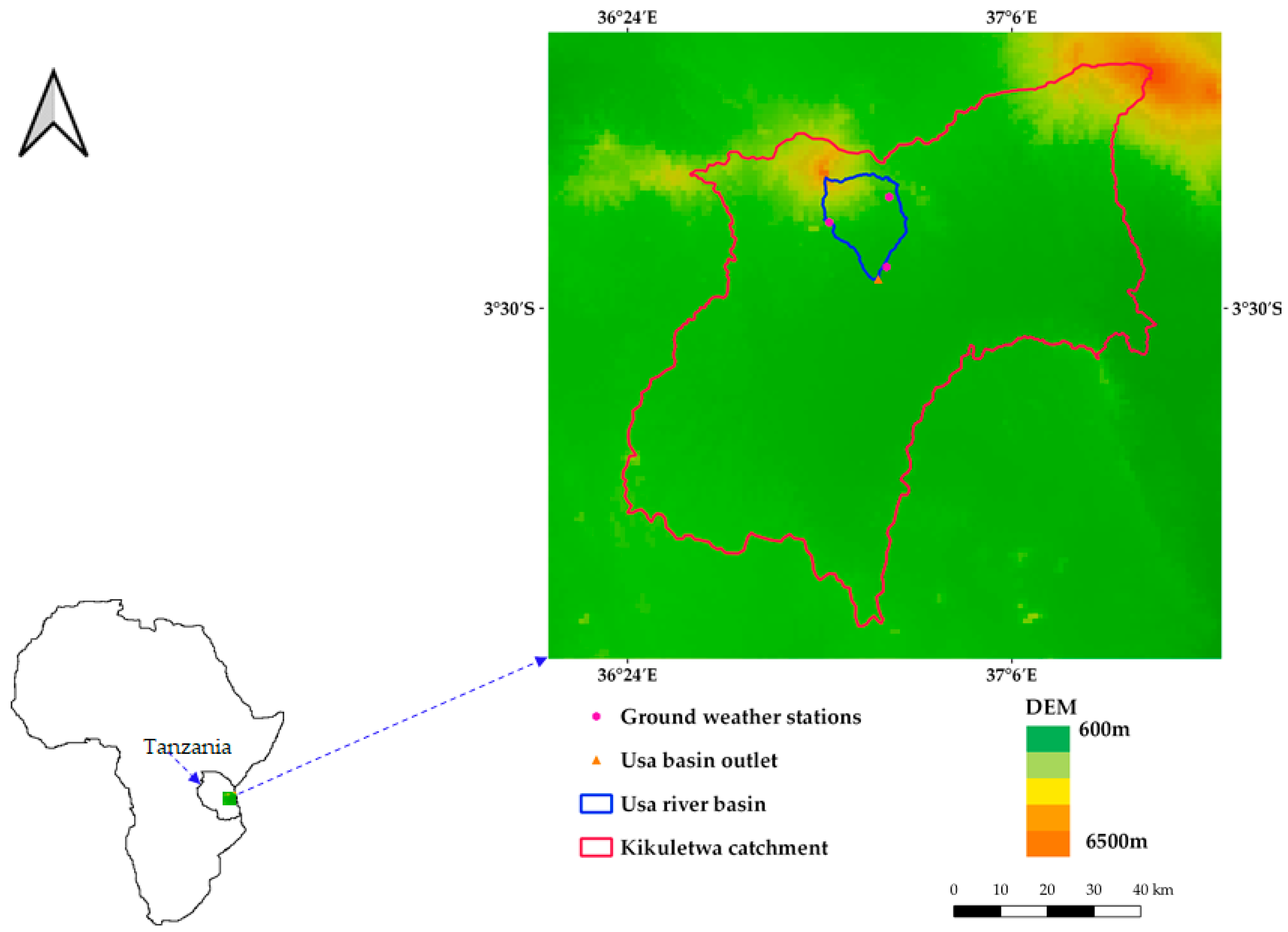
2.1. Case Study Description

The Kikuletwa river basin is in the western headwaters of the River Pangani and covers an area of 6765 km² with elevation ranging from 700 to 6000 m a.s.l. The Usa catchment, shown in Figure 1, within the Kikuletwa river basin was selected for this study. The Usa catchment covers an area of 240 km². The average rainfall within the basin ranges from 300 to 800 mm/year in the lower basin areas and 1200 to 2000 mm/year in the upper basin areas of the Meru and Kilimanjaro mountains [3]. Rainfall has a bimodal pattern, with rains occurring from March to May (Masika season) and rains occurring from November to December (Vuli season) [35]. The short rains in the Vuli season and the dry season are complemented with irrigation, using a traditional furrow system [36]. The maximum and minimum temperature ranges are 15 to 30 °C and 12 to 18 °C, respectively.

Land uses in the catchment include agricultural land, urban land, dense forests, grazed land, and shrubland. The dominant land-use types are rainfed and supplementary irrigated croplands, shrubland, and grassland [35]. The selection of the Usa catchment was based on the intensive agricultural activities taking place and the availability of seasonal land-use maps for March, August, and October 2016 [3].

2.2. Input Data

Data used for this study were obtained from different sources (local, national, and global datasets) and preprocessed, to make them usable for this study. Rainfall and temperature data from ground observation stations were collected from the Tanzania Meteorological Agency (TMA) for the period of 2006 through 2016. Three seasonal land-use maps for March, August, and October 2016 were obtained from [3]. However, the March and August maps had some unclassified pixels in the uplands which corresponded to the dense forest land-use pixels in the October map. These unclassified pixels were replaced with corresponding pixels from the October map, assuming that the dense forest land-use remains constant throughout the year. The soil map for the Usa catchment was obtained from FAO, SOTER (Soil and Terrain) database for Africa, at a coarse resolution of 1 km. The types of soils classified within the catchment were loam soil and clay loam soil. A Digital Elevation Model (DEM) that provides the physical characteristics of the study area was obtained from SRTM (Shuttle Radar Topography Mission), at a 30 m resolution.

2.3. SWAT and SWAT+ Models

SWAT is a semi-distributed river basin scale model that relies on the physical characteristics of a catchment. The model assesses impacts of different management decisions on water resources in watersheds with diverse land-use, soil, and management applications [37]. SWAT requires soil, weather, land-use, management, and topographic data for input irrespective of the application. However, management data, such as irrigation schedules, planting and harvesting dates, fertilization-application timings, and amounts, are the most challenging and difficult SWAT data to acquire and process [22].

SWAT+ is a revised version of SWAT that offers extra flexibility in connecting spatial units in the representation of management operations [11]. SWAT+ provides an improved simulation of landscape locations, overland routing, and floodplain processes. Land-use and management operations (e.g., irrigation, fertilization, and reservoir regulation) can be scheduled by using decision tables in SWAT+. This enables the user to add complex conditions during management scheduling, such as crop types or water availability in reservoirs, which is not possible in present models [38].

In both SWAT and SWAT+ models, the hydrological processes are represented by the variations in the HRUs consisting of unique land-use, slope, soil and management applications linked through a Geographic Information System (GIS) interface. In both models, a watershed is delineated into several sub-basins that are further subdivided into HRUs, using a GIS interface [39]. The models apply the water-balance concept as the basic driver of all hydrological processes in the catchment, as represented by Equation (1).

$${\mathrm{SW}}_{\mathrm{t}}={\mathrm{SW}}_{\mathrm{o}}+{{\displaystyle \sum }}^{}\left({\mathrm{V}}_{\mathrm{i}}-{\mathrm{Q}}_{\mathrm{i}}-{\mathrm{E}}_{\mathrm{i}}-{\mathrm{P}}_{\mathrm{i}}-{\mathrm{QR}}_{\mathrm{i}}\right)\times \mathsf{\Delta }\mathrm{t}$$

(1)

where ${\mathrm{SW}}_{\mathrm{t}}$ and ${\mathrm{SW}}_{\mathrm{o}}$ are the final and initial soil water content, respectively (mm/day); ${\mathrm{V}}_{\mathrm{i}}$ is the amount of precipitation (mm/day); ${\mathrm{Q}}_{\mathrm{i}}$ is the amount of surface runoff (mm/day); ${\mathrm{E}}_{\mathrm{i}}$ is the amount of ET (mm/day); ${\mathrm{P}}_{\mathrm{i}}$ is the amount of percolation (mm/day); ${\mathrm{QR}}_{\mathrm{i}}$ is the amount of return flow (mm/day); and Δt is change in time (day) and i is the index.

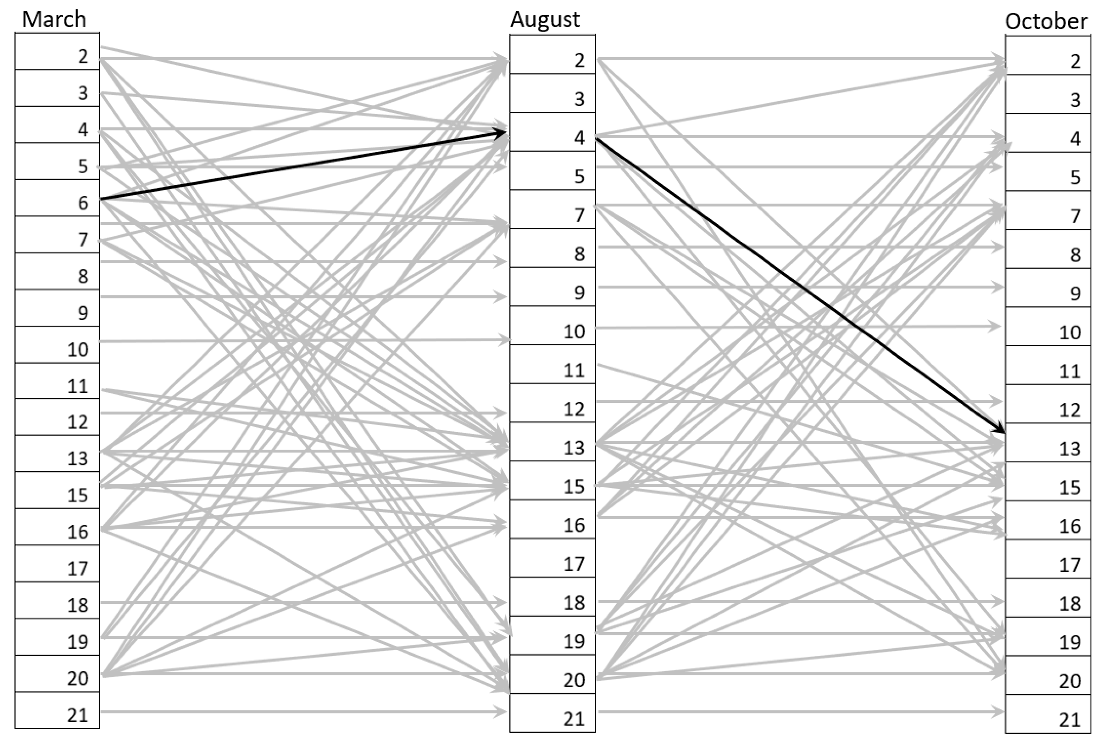
2.4. Land-Use Trajectory

All seasonal land-use maps were integrated in GIS, in a raster format, and land-use-trajectory change in Usa catchment was analyzed pixel by pixel, using the overlay analysis, as applied in [32]. Trajectories from the three land-use maps (March, August, and October) of Usa catchment were generated with the corresponding land-use codes described in

Table 1. Land use and the corresponding trajectory codes.

Land Use	Land-Use Code	Land Use	Land-Use Code
Water	1	grazed woodland	11
grazed shrubland	2	protected woodland	12
grazed grassland	3	irrigated mixed crops	13
bare land	4	irrigated banana and coffee	15
spare vegetation	5	irrigated banana, coffee and maize	16
rainfed maize	6	waterweed	17
irrigated sugarcane	7	urban buildings	18
afro-alpine forest	8	sparse vegetation or bare land	19
sub-alpine forest	9	shrubland or/and thickets	20
sub-alpine bushland	10	dense forest	21

and Figure 2. For example, as highlighted in Figure 2, a trajectory can be identified as 6 → 4→ 13, which means land-use changes from rainfed maize to bare land to irrigated mixed crops in March, August, and October maps, respectively. A total of 1160 trajectories were generated. However, some trajectories were unrealistic, such as a change from irrigated mixed crops land use in March to dense forest land use in August and to rainfed maize land use in October. These unrealistic trajectories, as well as the trajectories that took a small percentage of the overall trajectories, were excluded. Of the 1160 trajectories, the top 130 trajectories, covering about 90% of the whole catchment, were considered.

A distinction between static and dynamic trajectories was made, to characterize the seasonal changes in the land-use maps. The static trajectories are the continuous trajectories that remained constant in all the seasonal land-use maps, such as 21 → 21 → 21, corresponding to dense forest throughout the land-use maps, while the dynamic trajectories are the discontinuous trajectories that changed in the different seasonal land-use maps. There were 9 static trajectories that constituted 36.9% of the catchment and 121 dynamic trajectories that covered 53.4% of the catchment of the top 130 trajectories, indicating an intensive agricultural seasonal cycle throughout the year. The dominant static and dynamic trajectories are shown in

Table 2. The major static trajectories.

Dominant Static Trajectories	% Area to Static Trajectories
21 → 21 → 21	58.58
12 → 12 → 12	33.51
8 → 8 → 8	2.24
9 → 9 → 9	1.67
20 → 20 → 20	1.33

The numbers in the trajectories represent the land-use codes described in Table 1. The arrows signify a change from one land use to another.

and

Table 3. The major dynamic trajectories.

Dominant Dynamic Trajectories	% Area to Dynamic Trajectories
6 → 13 → 13	31.1
16 → 15 → 16	27.9
15 → 15 → 16	5.94
7 → 13 → 13	2.34
13 → 4→ 13	1.85

The numbers in the trajectories represent the land-use codes described in Table 1.

, respectively. Since the study’s focus was on the seasonal land-use dynamics, the top two dynamic trajectories in Table 3, 6 → 13 → 13 (rainfed maize to irrigated mixed crops to irrigated mixed crops) and 16 → 15 → 16 (irrigated banana, coffee and maize to irrigated banana and coffee to irrigated banana, coffee and maize), were selected for representation in the SWAT and SWAT+ models.

2.5. Model Configuration

Both SWAT and SWAT+ models were set up using the DEM, soil map, land-use map created for March 2016, and ground observation weather data of rainfall and temperature. Other weather parameters (wind speed, solar radiation, and humidity) were simulated by using an inbuilt weather generator in SWAT and SWAT+ models. The Climate Forecast System Reanalysis (CFSR) data [40,41], at a horizontal resolution of about 38 km, from 1979 to 2013, at a daily time step, were used in the SWAT weather generator, which has proved to be a valuable dataset in African data-scarce basins [42]. Due to the unavailability of several observed climate parameters, the Hargreaves method [43], which is temperature based, was selected to calculate the potential evapotranspiration. Within data-scarce East African catchments, the Hargreaves method has proved to give realistic estimations of PET [44]. The USDA Soil Conservation Service (SCS) curve number method was used to estimate surface runoff and variable storage method selected for flow routing in the channel.

No threshold was set for land use, soil, and slope during the HRU definition, so that all information about the catchment landscape could be captured. For the SWAT model, 9 sub-basins and 130 HRUs were generated, while for the SWAT+ model, 9 sub-basins, 9 landscape units, and 127 HRUs were generated in the default model setups. The differences in the number of HRUs could be attributed to the creation of HRUs through the sub-basins for the SWAT model, while the SWAT+ uses the landscape units to create the HRUs. However, both models generated 10 HRUs for the rainfed maize land use (Figure 3a) and 11 HRUs for the irrigated banana, coffee, and maize land use (Figure 3b), which were the HRUs of interest.

Both models (SWAT and SWAT+) were not calibrated but checked for water-balance estimations, as the study was not focusing on the simulation of flow but rather on improved representation of the crop and agricultural land-use dynamics in default model setups, which should in fact precede any calibration efforts. However, the BLAI (potential maximum leaf area index) for maize was adjusted to correspond with the field measurements made in the catchment.

2.6. Land-Use-Trajectory Implementation in the Models

2.6.1. Management Schedule Overview in Usa Catchment

In the Usa catchment, agricultural land uses follow different cropping patterns. The cropping calendar developed by Msigwa et al., [3] was adopted to aid the trajectory implementation by extracting the start and end periods of planting and harvesting for rainfed and irrigated crops.

2.6.2. Use of the Management File in SWAT

The SWAT management file was used to schedule the seasonal land-use trajectories, together with the corresponding management operations of irrigation and fertilization at the HRU level. Scheduling was done in calendar days, as opposed to heat units, since the cropping calendar was available.

For the rainfed maize to irrigated mixed crops to irrigated mixed crops (6 → 13 → 13) trajectory, a simplification of a generic agricultural land cover in SWAT with the plant code “AGRR” was used to represent the irrigated mixed crops, since the SWAT model only allows one crop at a time in an HRU [39,45]. Maize was represented by “CORN” plant code in the model.

Table 4. Operations schedule for the rainfed maize to irrigated mixed crops to irrigated mixed crops trajectory in SWAT.

Month	Day	Operation	Crop
1	22	Harvest and kill
3	15	Plant/begin growing season	CORN
3	17	Auto fertilization initialization
6	30	Harvest and kill
7	15	Plant/begin growing season	AGRR
7	17	Auto fertilization initialization
7	18	Auto irrigation initialization
9	30	Harvest and kill
10	7	Plant/begin growing season	AGRR
10	10	Auto fertilization initialization
10	11	Auto irrigation initialization

shows the implemented trajectory with the corresponding management schedule in the model. The irrigated banana, coffee, and maize to irrigated banana and coffee to irrigated banana, coffee, and maize (16 → 15 → 16) trajectory could not be represented in SWAT, because it had a cropping mixture of perennial crops (banana and coffee) and an annual crop (maize). Perennial crops keep a constant root structure during the year and do not need to be replanted every year, while the annual crops follow a single cropping season, from the plant date to the harvest date, within a year [20].

Both irrigation and fertilization operations were specified in the management file. Irrigation application in both the dry season and short rainy season was implemented through the auto-irrigation function in SWAT, using the soil-water-content method. This closely represents the actual field irrigation, where water is applied according to the water stress in the plant root zone [46]. Fertilization in SWAT was implemented through auto-fertilization, which applies nutrients when there is a level of nitrogen stress encountered by the plant. Urea fertilizer (Ammonium Nitrates) was specified, since it is the most used fertilizer in the Pangani basin [47], where the Usa catchment is located.

2.6.3. Use of Management Schedule and Decision Tables in SWAT+

Decision tables are a way of organizing and documenting complex events in a logical way that is easy to interpret [48]. In SWAT+, decision tables provide a specific way to model intricate sets of rules and their subsequent actions by allowing the user to add conditions for scheduling management actions [38]. In SWAT+, it was possible to implement both trajectories, including mixed cropping, because it is possible to simulate planting and harvesting of more than one crop in an HRU at a time if the crops are specified in the same plant community.

The planting and harvesting schedules for the rainfed maize to irrigated mixed crops to irrigated mixed crops trajectory and irrigated banana, coffee, and maize to irrigated banana and coffee to irrigated banana, coffee, and maize trajectory are presented in Appendix A,

Table A1. Planting and harvesting schedule for the rainfed maize to irrigated mixed crops to irrigated mixed crops trajectory in SWAT+ decision table.

Month	Day	Operation	Crop
1	20	Harvest and kill	CORN 1
3	15	Plant	CORN
6	29	Harvest and kill	CORN
7	14	Plant	TOMA 2
7	14	Plant	EGGP 3
9	29	Harvest and kill	TOMA
9	29	Harvest and kill	EGGP
10	6	Plant	CORN
10	6	Plant	TOMA
10	6	Plant	EGGP
12	16	Harvest and kill	TOMA
12	16	Harvest and kill	EGGP

¹ Plant code for maize; ² plant code for tomatoes; ³ plant code for eggplants.

and

Table A2. Planting and harvesting schedule for the irrigated banana, coffee, and maize to irrigated banana and coffee to irrigated banana, coffee, and maize trajectory in SWAT+ decision table.

Month	Day	Operation	Crop
1	22	Harvest and kill	CORN
3	15	Plant/begin growing season	CORN
6	30	Harvest and kill	CORN
7	7	Harvest	BANA 1
9	25	Harvest	BANA
9	30	Harvest	COFF 2
10	7	Plant/begin growing season	CORN
12	31	Harvest	BANA

¹ Plant code for bananas; ² plant code for coffee.

, respectively. The same parameters for auto-fertilization and auto-irrigation as applied in SWAT were applied in SWAT+, using decision tables in

Table 5. Decision table for irrigation application in SWAT+ for the rainfed maize to irrigated mixed crops to irrigated mixed crops trajectory.

Name	Conds	Alts	Acts
irr_corn 1	5	2	1
var	obj	obj_num	lim_var	lim_op	lim_const		alt1	alt2
w_stress	hru	0	null	−	0.8		<	<
jday	hru	0	null	−	195		>	−
jday	hru	0	null	−	272		<	−
jday	hru	0	null	−	279		−	>
jday	hru	0	null	−	365		−	<
act_typ	obj	obj_num	name	option	const	const2	fp	outcome
irr_demand 2	hru	0	furrow_irr 3	furrow 4	20.0	0.0	unlim 5	y y

Where; name = name of decision table, conds = number of conditions, alts = condition alternatives, acts = number of actions, var = variables, obj = objects, obj_num = object number, lim_var = limit variable, lim_op = limit operator, lim_const = limit constant, alt1 and alt2 = alternatives, w_stress = water stress variable, jday = Julian day, hru = HRU object, option = action option specific to type of action, const and const2 = constants used for amounts, fp = pointer for option, outcome = action outcomes, ¹ name assigned to decision table, ² name of the action type, ³ name of action, ⁴ name of option (furrow irrigation), ⁵ water from unlimited source.

,

Table 6. Decision table for irrigation application in SWAT+ for the irrigated banana, coffee, and maize to irrigated banana and coffee to irrigated banana, coffee, and maize trajectory.

Name	Conds	Alts	Acts
irr_bana 1	7	3	1
var	obj	obj_num	lim_var	lim_op	lim_const		alt1	alt2	alt3
w_stress	hru	0	null	−	0.8		<	<	<
jday	hru	0	null	−	73		>	-	−
jday	hru	0	null	−	180		<	>	−
jday	hru	0	null	−	195		−	<	−
jday	hru	0	null	−	272		−	−	−
jday	hru	0	null	−	279		−	−	>
jday	hru	0	null	−	365		−	−	<
act_typ	obj	obj_num	name	option	const	const2	fp	outcome
irr_demand	hru	0	furrow_irr	furrow	20.0	0.0	unlim	y y y

¹ name assigned to the decision table, for the other variable meanings, refer to Table 5 above.

and

Table 7. Decision table for fertilization application in SWAT+ for both trajectories.

Name	Conds	Alts	Acts
fert_mixed 1	7	3	1
var	obj	obj_num	lim_var	lim_op	lim_const		alt1	alt2	alt3
jday	hru	0	null	−	73		>	-	−
jday	hru	0	null	−	180		<	-	−
jday	hru	0	null	−	195		−	>	−
jday	hru	0	null	−	272		−	<	−
jday	hru	0	null	−	279		−	−	>
jday	hru	0	null	−	365		−	−	<
n_stress	hru	0	null	−	0.8		<	<	<
act_typ	obj	obj_num	name	type	const	const2	application outcome
fertilize 2	hru	0	Urea_fert 3	urea 4	40.0	0.0	broadcast 5 y y y

¹ name of the decision table, ² name of the action type (fertilize), ³ name of the action, ⁴ type of option (urea fertilizer), ⁵ broadcast application mode of fertilizer, for other variable meanings, refer to Table 5.

, for both trajectories to maintain consistency in both models. The conditional variables used in the decision tables, currently coded in SWAT+, are well defined and elaborated by Arnold et al., [38].

In Table 5, an irrigation application of 20 mm for the rainfed maize to irrigated mixed crops to irrigated mixed crops trajectory was triggered when the water stress was less that 0.8 of the soil Field Capacity (FC) in the dry season (between day 195 and 272) and the short rainy season (between day 279 and 365). For the irrigated banana, coffee, and maize to irrigated banana and coffee to irrigated banana, coffee, and maize trajectory in Table 6, the same conditions were set, in addition to the irrigation application in the first planting season (between day 73 and 180). In Table 7, the nitrogen stress threshold was set at 0.8, and fertilizer was applied by the model to the HRU, when actual plant growth fell below the threshold. A maximum amount of 40 kg/ha of Urea fertilizer was specified in any one application within the growing seasons (i.e., day 73 to 180; day 195 to 272; and day 279 to 365).

2.7. SWAT and SWAT+ Model Evaluation

It is worth keeping in mind that the overall aim of these simulations is to show inconsistences in the default simulations of agricultural land-use dynamics in African catchments. Hence, the focus was on how representation of temporal dynamics (seasonal trends) of LAI vegetative growth correlate with the seasonal weather patterns in default model setups. LAI model outputs were compared with remote-sensing LAI products, to evaluate the performance of the SWAT and SWAT+ models in simulating land-use trajectories. Alemayehu et al., [15] has expressed the importance of using remote-sensing LAI products for evaluating SWAT model outputs, especially in cases with limited data availability. TREX (Tool for Raster data Exploration) (https://github.com/VUB-HYDR/TREX) [49] was used to process daily PROBA-V satellite images (http://proba-v.vgt.vito.be/en) [50] of the Normalized Differential Vegetation Index (NDVI) at 1 km resolution into LAI images and monthly time series. TREX uses the following universal equation by [51], to calculate the LAI:

$$\mathrm{LAI}=\sqrt{\mathrm{NDVI}\frac{\left(1+\mathrm{NDVI}\right)}{\left(1-\mathrm{NDVI}\right)}}$$

(2)

The Spearman correlation coefficient analysis that has been applied in previous studies [52] was done between the models’ LAI outputs and the LAI from TREX, to measure the extent to which the variables change together (significance of relationship) in both the default and trajectory models. The Spearman rank correlation is a non-parametric rank that measures the association between two variable sequences [53]. This monotonic function is as follows:

$$R=1-\frac{6{{\displaystyle \sum }}^{}{d}^2}{n\left(n^2-1\right)}$$

(3)

where R denotes the Spearman rank correlation coefficient, d is the difference between the sequences, and n is the number of sequences. The Spearman rank correlation, R, will always be between 1.0 (perfect positive correlation) and −1.0 (perfect negative correlation). Furthermore, the measure of how likely or probable it is that any observed correlation is due to chance (p-value) was also calculated based on the R value and sample size. This value ranges between 0 and 1. A p-value close to 1 suggests that the correlation is most likely due to chance, while a p-value close to 0 suggests that the observed correlation is unlikely to be due to chance [54].

3. Results and Discussion

3.1. Water-Balance Check

Comparison of the water-balance components was carried out at the HRU level for both the default SWAT and SWAT+ models, as well as the implemented trajectories in the models, as shown in

Table 8. Comparison of the water-balance components in SWAT, at the HRU level.

Water Balance Component (mm)	Default Model	Rainfed Maize Trajectory Model
Precipitation	744.2	744.2
Irrigation	-	209.0
Evaporation	492.8	688.8
Lateral flow	5.9	2.5
Surface runoff	183.7	185.4
Percolation	90.0	66.4
Mass balance	−28.2	10.1

and

Table 9. Comparison of the water-balance components in SWAT+ at HRU level.

Water Balance Components (mm)	Irrigated Banana, Coffee, and Maize HRUs		Rainfed Maize HRUs
	Default Model	Trajectory Model	Default Model	Trajectory Model
Precipitation	811.0	811.0	811.0	811.0
Irrigation	-	235.2	-	293.5
Evaporation	589.1	690.5	479.0	700.4
Lateral flow	4.8	12.9	4.8	11.8
Surface runoff	20.8	28.9	30.8	21.3
Percolation	201.8	311.2	296.9	372.4
Mass balance	−5.5	−2.7	−0.5	−1.4

, respectively. The precipitation in the SWAT+ model in Table 9 was slightly different from the precipitation in the SWAT model in Table 8, even though the same parameters were used during the different model setups. This can be attributed to the way precipitation stations are allocated in the different models. In SWAT, precipitation stations are allocated based on the sub-basins, while in SWAT+, this is done based on the landscape units. There was also a difference of 83% in surface runoff and 67% in deep percolation between the SWAT and SWAT+ default models, highlighting the uncertainties in the two model structures.

Except for precipitation, all water-balance components in Table 8 and Table 9 changed after the implementation of the trajectories. Notably, ET increased significantly in both models, as observed in Figure 4. In the SWAT model, ET increased by 40% for the rainfed maize to irrigated mixed crops to irrigated mixed crops trajectory, while in the SWAT+ model, ET increased by 17% and 46% after the implementation of the irrigated banana, coffee, and maize to irrigated banana and coffee to irrigate banana, coffee, and maize trajectory and the rainfed maize to irrigated mixed crops to irrigated mixed crops trajectory, respectively. The increase in ET highlights the impact of including agricultural seasonal land-use dynamics in the model on the water balance.

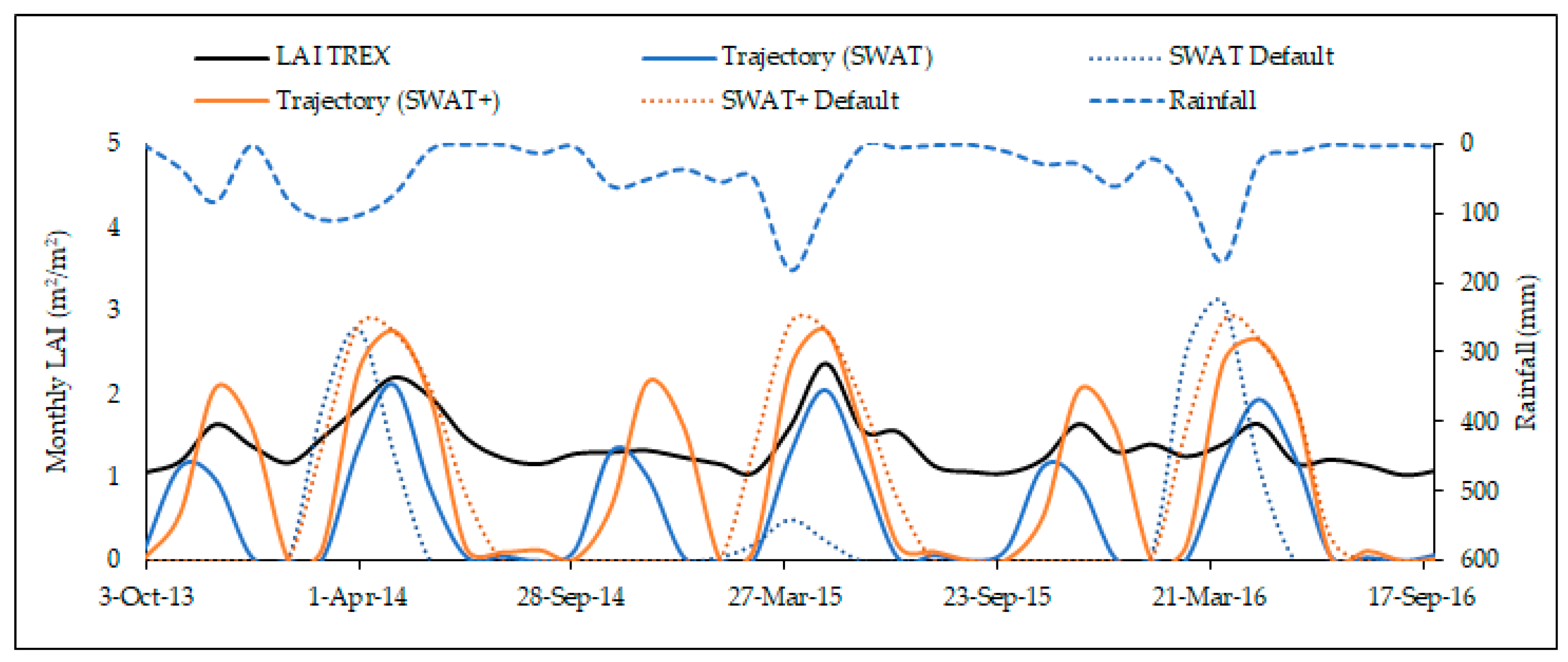
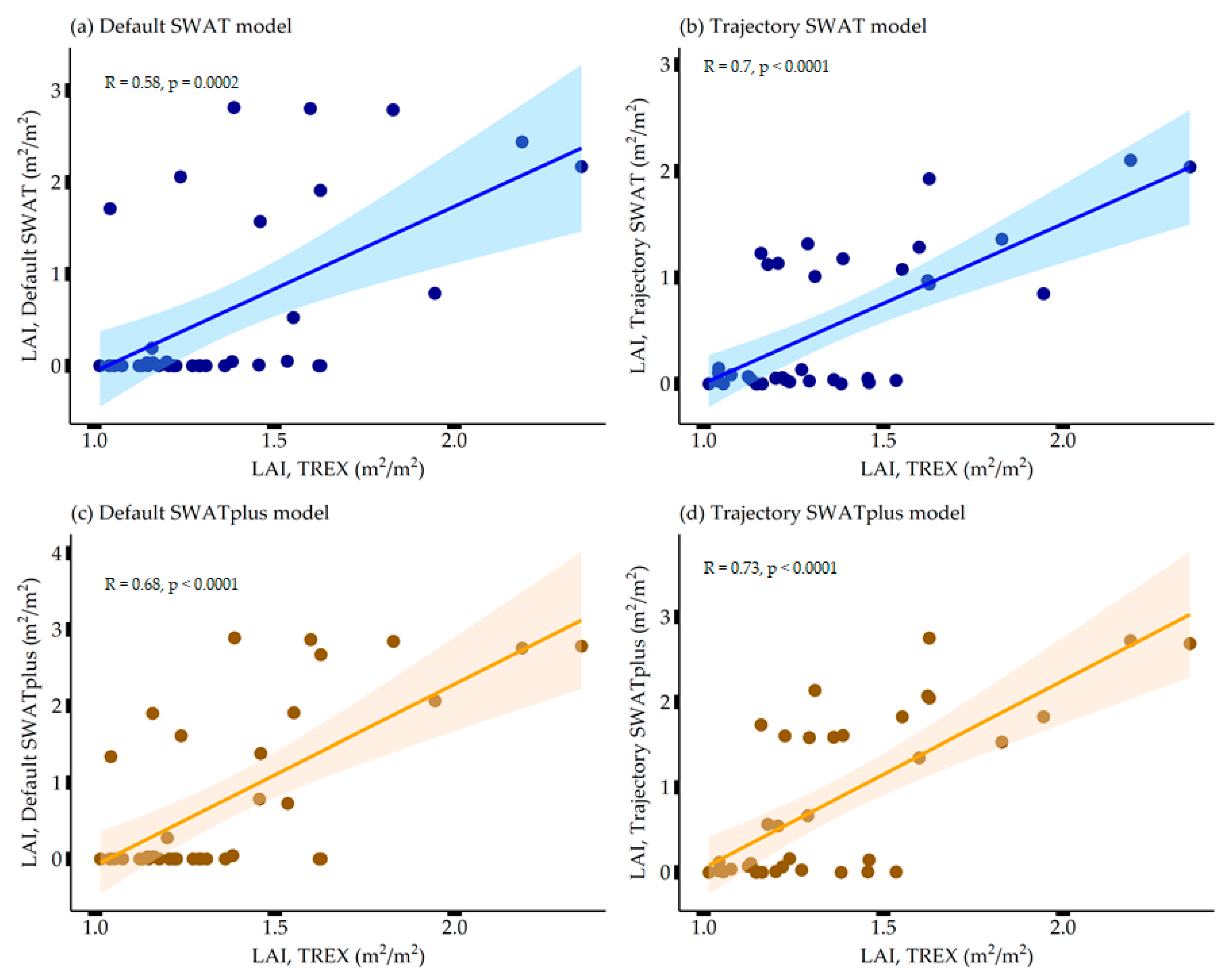
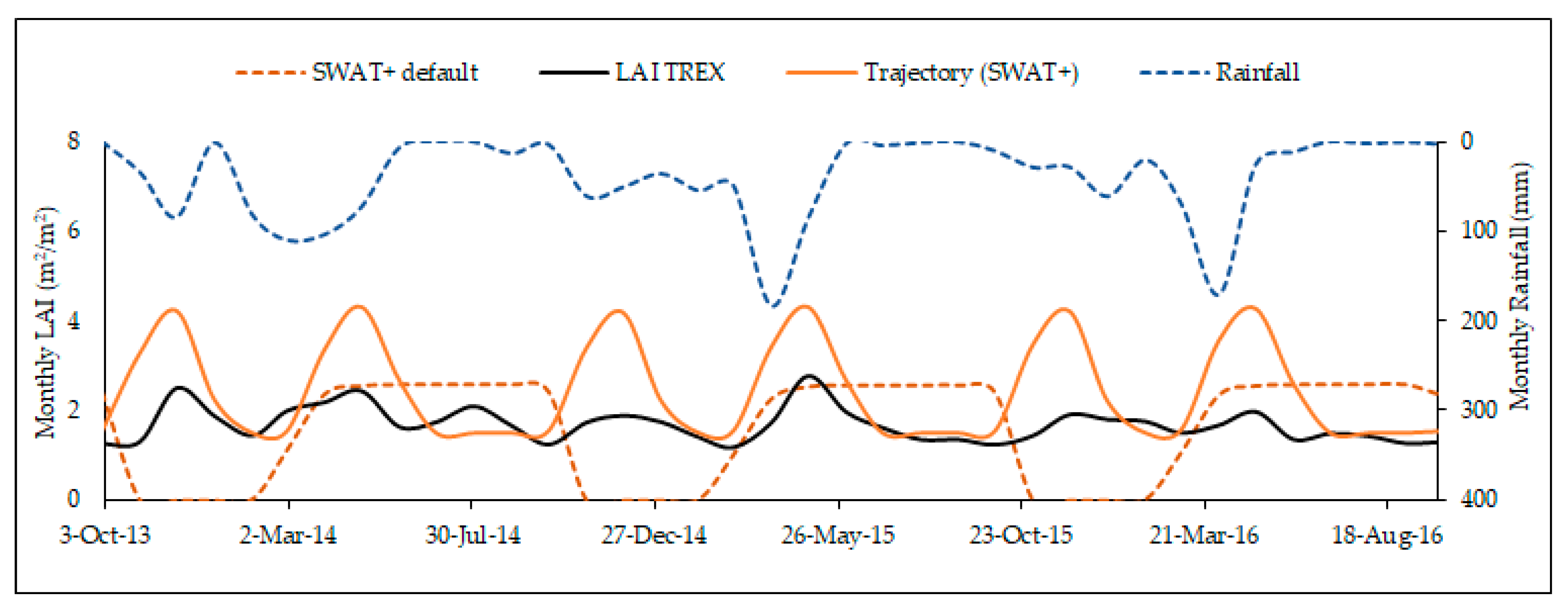
3.2. Leaf Area Index Comparison

It should be noted that the remote-sensing LAI values were obtained at a 1 km resolution, meaning that they capture different vegetation and cannot be treated as a pure signal of a single crop. However, they provide an insight on the temporal crop-growth relationship to dry and wet seasonal patterns, and catchment management practices, which provides a way for identifying model simulation inaccuracies in crop phenology.

3.2.1. Rainfed Maize to Irrigated Mixed Crops to Irrigated Mixed Crops Trajectory

In Figure 5, both the default SWAT and SWAT+ model LAI values for rainfed maize land use depict only one growing season (March to July) throughout the year. This contradicts the remote-sensing LAI values that depict two major growing seasons corresponding with the two rainy seasons of March to May and November to December. Furthermore, the remote-sensing LAI values do not drop to zero throughout the year, while in SWAT and SWAT+ models, the values drop to zero after the first growing season. In SWAT and SWAT+ models, the crop LAI drops to zero because of the ‘harvest and kill’ operation, but in reality, there is more vegetation, such as shrubs or trees, surrounding the fields, which may remain green after harvesting the crops. For that reason, a remote-sensing LAI signal will not go to zero, as compared to the LAI from the crop HRU simulated in SWAT and SWAT+ models between the growing seasons.

During the first growing season, the default SWAT and SWAT+ models LAI values were higher than the remote-sensing LAI by TREX in Figure 5, since the default models simulate LAI of one single crop, while remote-sensing products average all vegetation, and possibly bare land, in a pixel, due to a coarse resolution. In addition, auto-fertilization is applied during the default simulation, and the model applies enough fertilizer to meet harvest removal, as well as an additional amount to compensate for any nitrogen losses to surface runoff or leaching [39]. However, this does not reflect real fertilization practices. Van Griensven et al., [55] also highlighted an overestimation of LAI by a SWAT model in comparison with remote-sensing data.

Both trajectory implementations in SWAT and SWAT+ models capture the two major growing seasons within the two rainy seasons, as the LAI increases between the seasons, following the TREX LAI pattern in Figure 5. The correlation between the trajectory LAI and TREX LAI slightly increased in Figure 6b,d for both model implementations, signifying an improved relationship. The slight increase in correlation can be attributed to the implementation of the seasonal land-use trajectories in the model, giving LAI patterns that captures the two growing seasons corresponding to the TREX LAI vegetative growth patterns. However, the LAI of the trajectory simulations dropped to zero in February and September, which are dry months in the catchment [7], unlike the TREX LAI that does not drop to zero. This reflects the inclusion of other vegetation within the TREX LAI pixel that are averaged together rather than representing a single crop as simulated by the SWAT and SWAT+ models. This shows the complexity and scaling issues when using remote-sensing products in model evaluation at the HRU level.

3.2.2. Irrigated Banana, Coffee, and Maize to Irrigated Banana and Coffee to Irrigated Banana, Coffee, and Maize Trajectory

The default SWAT+ LAI was at a maximum constant for seven months, every year, throughout the simulated growing period (Figure 7), which does not reflect real crop practices in Usa catchment. The constant LAI can be attributed to using a perennial land cover (banana) in SWAT+ to represent the irrigated banana, coffee, and maize land use during the default model set up. The LAI of the default SWAT+ model falls to zero in November until January, following dormancy, whereby the default growing season in the model goes from January until October, which is not realistic for agricultural crops in Usa catchment.

From Figure 8a, there is no existing relationship between the default SWAT+ model LAI output and the remote-sensing reference LAI. However, there is a strong correlation between the trajectory model LAI and the remote-sensing LAI (Figure 8b). This result is consistent with the irrigated banana, coffee, and maize to irrigated banana and coffee to irrigated banana, coffee, and maize trajectory capturing the major growing seasons corresponding with the rainy seasons. It is also good to note that the trajectory LAI does not fall to zero, which is representative of perennial crops.

4. Conclusions

In this study, we present an innovative approach of representing the seasonal land-use dynamics of the Usa catchment in the Kikuletwa basin in SWAT and SWAT+ models, based on land-use trajectories. The impact of these representations was assessed by comparing the SWAT and SWAT+ model outputs with remote-sensing LAI products. The results indicated an improved vegetation simulation by the models in cultivated catchments following clear dry and wet seasons. The LAI dynamics of the trajectory implementations showed more realistic temporal advancement patterns that corresponded to the seasonal rainfall within the catchment and in agreement with the remote sensing products, as compared to the default model setups.

The principal change to the default models that use land-use and land-cover (LULC) maps was the manual implementation of the seasonal land-use dynamics, which was done by linking the land-use trajectories to the LULC maps. The dominant dynamic trajectories were implemented in SWAT and SWAT+, using a management file and decision tables, respectively. The decision tables in SWAT+ provided more flexibility, as mixed cropping in the same HRU at the same time was possible, unlike in SWAT.

Although the representation of the seasonal land-use dynamics through land-use trajectories can be challenging, involving numerous manual edits as compared to a static representation through land cover classes, representing land-use dynamics improves the model representation of LAI. Especially for regions that are intensively cultivated with several cropping seasons, the model is able to reflect the seasonal patterns of vegetative growth simulations in correspondence to the seasonal weather. This is the first study dealing with dynamic land-use representation by using land-use trajectories for cultivated tropical catchments in hydrological models. Hence, this is a critical step toward more realistic hydrological modeling applications of SWAT and SWAT+ default models in African cultivated catchments with multiple growing seasons within a year.

References

1. Maletta, H.E. Land and farm production: Availability, use, and productivity of agricultural land in the world. SSRN Electron. J. 2014. [Google Scholar] [CrossRef] [Green Version]
2. Barrios, S.; Ouattara, B.; Strobl, E. The impact of climatic change on agricultural production: Is it different for Africa? Food Policy 2008, 33, 287–298. [Google Scholar] [CrossRef] [Green Version]
3. Msigwa, A.; Komakech, H.C.; Verbeiren, B.; Salvadore, E.; Hessels, T.; Weerasinghe, I.; van Griensven, A. Accounting for seasonal land use dynamics to improve estimation of agricultural irrigation water withdrawals. Water 2019, 11, 2471. [Google Scholar] [CrossRef] [Green Version]
4. Verburg, P.H.; Schot, P.P.; Dijst, M.J.; Veldkamp, A. Land use change modelling: Current practice and research priorities. Geo J. 2004, 61, 309–324. [Google Scholar] [CrossRef]
5. Boddy, P.L.; Baker, J.L. Conservation Tillage Effects on Nitrate and Atrazine Leaching; Paper 90-2503; American Society of Agricultural Engineers: St. Joseph, MI, USA, 1990; pp. 90–2503. [Google Scholar]
6. Weed, D.A.J.; Kanwar, R.S. Nitrate and water present in and flowing from root-zone soil. J. Environ. Qual. 1996, 25, 709–719. [Google Scholar] [CrossRef]
7. Munishi, L.K.; Sawere, P.C. Climate change and decline in water resources in Kikuletwa Catchment, Pangani, northern Tanzania. Afr. J. Environ. Sci. Technol. 2014, 8, 58–65. [Google Scholar] [CrossRef] [Green Version]
8. Dakhlalla, A.O.; Parajuli, P.B.; Ouyang, Y.; Schmitz, D.W. Evaluating the impacts of crop rotations on groundwater storage and recharge in an agricultural watershed. Agric. Water Manag. 2016, 163, 332–343. [Google Scholar] [CrossRef] [Green Version]
9. Lambin, E.F.; Rounsevell, M.D.A.; Geist, H.J. Are agricultural land-use models able to predict changes in land-use intensity? Agric. Ecosyst. Environ. 2000, 82, 321–331. [Google Scholar] [CrossRef]
10. Arnold, J.G.; Srinivasan, R.; Muttiah, R.S.; Williams, J.R. Large area hydrologic modeling and assessment part I: Model development1. JAWRA J. Am. Water Resour. Assoc. 1998, 34, 73–89. [Google Scholar] [CrossRef]
11. Bieger, K.; Arnold, J.G.; Rathjens, H.; White, M.J.; Bosch, D.D.; Allen, P.M.; Volk, M.; Srinivasan, R. Introduction to SWAT+, a completely restructured version of the soil and water assessment tool. JAWRA J. Am. Water Resour. Assoc. 2017, 53, 115–130. [Google Scholar] [CrossRef]
12. Gassman, P.; Reyes, M.; Green, C.; Arnold, J. The soil and water assessment tool: Historical development, applications, and future research directions. Trans. ASABE 2007, 1211–1250. [Google Scholar] [CrossRef] [Green Version]
13. Farjad, B.; Gupta, A.; Razavi, S.; Faramarzi, M.; Marceau, D.J. An integrated modelling system to predict hydrological processes under climate and land-use/cover change scenarios. Water 2017, 9, 767. [Google Scholar] [CrossRef] [Green Version]
14. Van Griensven, A.; Ndomba, P.; Yalew, S.; Kilonzo, F. Critical review of SWAT applications in the upper Nile basin countries. Hydrol. Earth Syst. Sci. 2012, 16, 3371–3381. [Google Scholar] [CrossRef] [Green Version]
15. Alemayehu, T.; van Griensven, A.; Woldegiorgis, B.T.; Bauwens, W. An improved SWAT vegetation growth module and its evaluation for four tropical ecosystems. Hydrol. Earth Syst. Sci. 2017, 21, 4449–4467. [Google Scholar] [CrossRef] [Green Version]
16. Easton, Z.M.; Fuka, D.R.; White, E.D.; Collick, A.S.; Biruk Ashagre, B.; McCartney, M.; Awulachew, S.B.; Ahmed, A.A.; Steenhuis, T.S. A multi basin SWAT model analysis of runoff and sedimentation in the Blue Nile, Ethiopia. Hydrol. Earth Syst. Sci. 2010, 14, 1827–1841. [Google Scholar] [CrossRef] [Green Version]
17. Parajuli, P.B.; Jayakody, P.; Sassenrath, G.F.; Ouyang, Y.; Pote, J.W. Assessing the impacts of crop-rotation and tillage on crop yields and sediment yield using a modeling approach. Agric. Water Manag. 2013, 119, 32–42. [Google Scholar] [CrossRef]
18. Gao, J.; Sheshukov, A.Y.; Yen, H.; Kastens, J.H.; Peterson, D.L. Impacts of incorporating dominant crop rotation patterns as primary land use change on hydrologic model performance. Agric. Ecosyst. Environ. 2017, 247, 33–42. [Google Scholar] [CrossRef]
19. Karcher, S.C.; VanBriesen, J.M.; Nietch, C.T. Alternative land-use method for spatially informed watershed management decision making using SWAT. J. Environ. Eng. 2013, 139, 1413–1423. [Google Scholar] [CrossRef]
20. Neitsch, S.L.; Arnold, J.G.; Kiniry, J.R.; Williams, J.R. Soil and Water Assessment Tool Theoretical Documentation Version 2009; Texas Water Resources Institute: College Station, TX, USA, 2011. [Google Scholar]
21. Strauch, M.; Volk, M. SWAT plant growth modification for improved modeling of perennial vegetation in the tropics. Ecol. Model. 2013, 269, 98–112. [Google Scholar] [CrossRef]
22. White, M.; Gambone, M.; Yen, H.; Daggupati, P.; Bieger, K.; Deb, D.; Arnold, J. Development of a cropland management dataset to support U.S. swat assessments. JAWRA J. Am. Water Resour. Assoc. 2016, 52, 269–274. [Google Scholar] [CrossRef]
23. Donohue, R.J.; Roderick, M.L.; McVicar, T.R. On the importance of including vegetation dynamics in Budyko’s hydrological model. Hydrol. Earth Syst. Sci. Discuss. 2006, 3, 1517–1551. [Google Scholar] [CrossRef] [Green Version]
24. Wegehenkel, M. Modeling of vegetation dynamics in hydrological models for the assessment of the effects of climate change on evapotranspiration and groundwater recharge. Adv. Geosci. 2009, 21, 109–115. [Google Scholar] [CrossRef] [Green Version]
25. Zhang, X.; Friedl, M.A.; Schaaf, C.B.; Strahler, A.H.; Liu, Z. Monitoring the response of vegetation phenology to precipitation in Africa by coupling MODIS and TRMM instruments. J. Geophys. Res. Atmos. 2005, 110. [Google Scholar] [CrossRef]
26. Castillo, C.R.; Güneralp, İ.; Güneralp, B. Influence of changes in developed land and precipitation on hydrology of a coastal Texas watershed. Appl. Geogr. 2014, 47, 154–167. [Google Scholar] [CrossRef]
27. Ruiz, J.; Domon, G. Analysis of landscape pattern change trajectories within areas of intensive agricultural use: Case study in a watershed of southern Québec, Canada. Landsc. Ecol. 2009, 24, 419–432. [Google Scholar] [CrossRef]
28. Wagner, P.D.; Bhallamudi, S.M.; Narasimhan, B.; Kumar, S.; Fohrer, N.; Fiener, P. Comparing the effects of dynamic versus static representations of land use change in hydrologic impact assessments. Environ. Model. Softw. 2017. [Google Scholar] [CrossRef]
29. Wang, Q.; Liu, R.; Men, C.; Guo, L.; Miao, Y. Effects of dynamic land use inputs on improvement of SWAT model performance and uncertainty analysis of outputs. J. Hydrol. 2018, 563, 874–886. [Google Scholar] [CrossRef]
30. Kumar, E.; Saraswat, D.; Singh, G. Comparative analysis of bioenergy crop impacts on water quality using static and dynamic land use change modeling approach. Water 2020, 12, 410. [Google Scholar] [CrossRef] [Green Version]
31. Pai, N.; Saraswat, D. SWAT2009_LUC: A tool to activate the land use change module in SWAT 2009. Trans. ASABE 2011, 54, 1649–1658. [Google Scholar] [CrossRef]
32. Mertens, B.; Lambin, E.F. Land-cover-change trajectories in southern Cameroon. Ann. Assoc. Am. Geogr. 2000, 90, 467–494. [Google Scholar] [CrossRef]
33. Zhou, Q.; Li, B.; Kurban, A. Trajectory analysis of land cover change in arid environment of China. Int. J. Remote Sens. 2008, 29, 1093–1107. [Google Scholar] [CrossRef]
34. Wang, D.; Gong, J.; Chen, L.; Zhang, L.; Song, Y.; Yue, Y. Spatio-temporal pattern analysis of land use/cover change trajectories in Xihe watershed. Int. J. Appl. Earth Obs. Geoinf. 2012, 14, 12–21. [Google Scholar] [CrossRef]
35. Kiptala, J.K.; Mul, M.L.; Mohamed, Y.; Van der Zaag, P. Modelling stream flow and quantifying blue water using modified STREAM model in the Upper Pangani river basin, Eastern Africa. Hydrol. Earth Sys. Sci. Discuss. 2013, 10. [Google Scholar] [CrossRef]
36. Munishi, P.K.T.; Hermegast, A.M.; Mbilinyi, B.P. The impacts of changes in vegetation cover on dry season flow in the Kikuletwa River, northern Tanzania. Afr. J. Ecol. 2009, 47, 84–92. [Google Scholar] [CrossRef]
37. Arnold, J.G.; Moriasi, D.N.; Gassman, P.W.; Abbaspour, K.C.; White, M.J.; Srinivasan, R.; Santhi, C.; Harmel, R.D.; Van Griensven, A.; Van Liew, M.W. SWAT: Model use, calibration, and validation. Trans. ASABE 2012, 55, 1491–1508. [Google Scholar] [CrossRef]
38. Arnold, J.; Bieger, K.; White, M.; Srinivasan, R.; Dunbar, J.; Allen, P. Use of decision tables to simulate management in SWAT+. Water 2018, 10, 713. [Google Scholar] [CrossRef] [Green Version]
39. Arnold, J.G.; Kiniry, J.R.; Srinivasan, R.; Williams, J.R.; Haney, E.B.; Neitsch, S.L. SWAT 2012 Input/Output Documentation; Texas Water Resources Institute: College Station, TX, USA, 2013. [Google Scholar]
40. Dile, Y.T.; Srinivasan, R. Evaluation of CFSR climate data for hydrologic prediction in data-scarce watersheds: An application in the Blue Nile river basin. JAWRA J. Am. Water Resour. Assoc. 2014, 50, 1226–1241. [Google Scholar] [CrossRef]
41. Fuka, D.R.; Walter, M.T.; MacAlister, C.; Degaetano, A.T.; Steenhuis, T.S.; Easton, Z.M. Using the climate forecast system reanalysis as weather input data for watershed models. Hydrol. Process. 2014, 28, 5613–5623. [Google Scholar] [CrossRef]
42. Tolera, M.B.; Chung, I.-M.; Chang, S.W. Evaluation of the climate forecast system reanalysis weather data for watershed modeling in upper Awash basin, Ethiopia. Water 2018, 10, 725. [Google Scholar] [CrossRef] [Green Version]
43. Hargreaves, G.H.; Samani, Z.A. Reference crop evapotranspiration from temperature. Appl. Eng. Agric. 1985, 1, 96–99. [Google Scholar] [CrossRef]
44. Alemayehu, T.; van Griensven, A.; Bauwens, W. Evaluating CFSR and WATCH data as input to SWAT for the estimation of the potential evapotranspiration in a data-scarce eastern-African catchment. J. Hydrol. Eng. 2016, 21. [Google Scholar] [CrossRef]
45. Kiniry, J.R.; Macdonald, J.D.; Kemanian, A.R.; Watson, B.; Putz, G.; Prepas, E.E. Plant growth simulation for landscape-scale hydrological modelling. Hydrol. Sci. J. 2008, 53, 1030–1042. [Google Scholar] [CrossRef] [Green Version]
46. Chen, Y.; Marek, G.; Marek, T.; Brauer, D.; Srinivasan, R. Assessing the efficacy of the SWAT auto-irrigation function to simulate irrigation, evapotranspiration, and crop response to management strategies of the Texas high plains. Water 2017, 9, 509. [Google Scholar] [CrossRef]
47. Benson, T.; Kirama, S.L.; Selejio, O. The Supply of Inorganic Fertilizers to Smallholder Farmers in Tanzania: Evidence for Fertilizer Policy Development; International Food Policy Research Institute (IFPRI): Washington, DC, USA, 2012. [Google Scholar] [CrossRef] [Green Version]
48. Metzner, J.R.; Barnes, B.H. Decision Table Languages and Systems; Academic Press: Cambridge, MA, USA, 2014. [Google Scholar]
49. Suliga, J.; Bhattacharjee, J.; Chormański, J.; van Griensven, A.; Verbeiren, B. Automatic proba-V processor: TREX—Tool for Raster Data Exploration. Remote Sens. 2019, 11, 2538. [Google Scholar] [CrossRef] [Green Version]
50. Wolters, E.; Dierckx, W.; Dries, J.; Swinnen, E. PROBA-V Products User Manual. 2014. Available online: http://proba-v.vgt.vito.be/sites/proba-v.vgt.vito.be/files/products_user_manual.pdf (accessed on 20 March 2019).
51. Su, Z. Remote Sensing Applied to Hydrology: The Sauer River Basin Study. Ph.D. Thesis, Faculty of Civil Engineering, Ruhr University Bochum, Bochum, Germany, 1996. [Google Scholar]
52. Coutu, G.; Vega Orozco, C. Impacts of landuse changes on runoff generation in the east branch of the Brandywine creek watershed using a GIS-based hydrologic model. Middle States Geogr. 2007, 40, 142–149. [Google Scholar]
53. Liu, D.; Cho, S.-Y.; Sun, D.-M.; Qiu, Z.-D. A Spearman correlation coefficient ranking for matching-score fusion on speaker recognition. In Proceedings of the TENCON 2010–2010 IEEE Region 10 Conference, Fukuoka, Japan, 21–24 November 2010; pp. 736–741. [Google Scholar] [CrossRef]
54. Akoglu, H. User’s guide to correlation coefficients. Turk J. Emerg. Med. 2018, 18, 91–93. [Google Scholar] [CrossRef]
55. Van Griensven, A.; Maskey, S.; Stefanova, A. The use of satellite images for evaluating a SWAT model: Application on the Vit Basin, Bulgaria. In Proceedings of the 6th International Congress on Environmental Modeling and Software, Leipzig, Germany, 1–5 July 2012. [Google Scholar]
Figure 1. Location of Usa catchment within Kikuletwa river basin.
Water 12 01541 g001
Figure 2. Land-use trajectories in the Usa catchment, Tanzania.
Water 12 01541 g002
Figure 3. (a) HRUs for implementation of rainfed maize to irrigated mixed crops to irrigated mixed crops trajectory and (b) HRUs for the implementation of irrigated banana, coffee, and maize to irrigated banana and coffee to irrigated banana, coffee, and maize trajectory.
Water 12 01541 g003
Figure 4. (a) ET at HRU level in default SWAT model; (b) ET at HRU level in default SWAT+ model; (c) ET at HRU level after implementation of trajectories in the SWAT model; (d) ET at HRU level after implementation of trajectories in SWAT+ model.
Water 12 01541 g004
Figure 5. LAI comparison of the rainfed-maize land use for default and trajectory implementation.
Water 12 01541 g005
Figure 6. Correlation analysis between TREX LAI and SWAT and SWAT+ default models and rainfed maize to irrigated mixed crops to irrigated mixed crops trajectory outputs.
Water 12 01541 g006
Figure 7. LAI comparison of the irrigated banana, coffee, and maize land use, default and trajectory implementation in SWAT+.
Water 12 01541 g007
Figure 8. Correlation analysis between TREX LAI and SWAT+ default models and irrigated banana, coffee, and maize to irrigated banana and coffee to irrigated banana, coffee, and maize trajectory outputs.
Water 12 01541 g008