New Pond—Indicator Bacteria to Complement Routine Monitoring in a Wet/Dry Tropical Wastewater Stabilization System

Abstract

Bacteria monitoring is a critical part of wastewater management. At tropical wastewater stabilization ponds (WSPs) in north Australia, sanitation is assessed using the standard fecal indicator bacteria (FIB) Escherichia coli and Enterococci. However, these bacteria are poor surrogates for enteric pathogens. A focus on FIB misses the majority of pond-bacteria and how they respond to the tropical environment. Therefore, we aimed to identify the unknown pond bacteria and indicators that can complement E. coli to improve monitoring. Over two years, we measured the bacterial community in 288 wastewater samples during the wet and dry seasons. The WSP community was spatially and temporally dynamic. Standard pond-water physicochemical measures like conductivity poorly explained these community shifts. Cyanobacteria represented >6% of the WSP bacterial population, regardless of sample timing and location. Fecal bacteria were abundant in the first pond. However, in downstream ponds, these bacteria were less abundant, and instead, environmental taxa were common. For each pond, we identified a bacterial fingerprint that included new candidate bacterial indicators of fecal waste and processes like nitrogen removal. Combining the new indicators with standard FIB monitoring represents a locally relevant approach to wastewater monitoring that facilitates new tests for human fecal pollution within tropical climates.

1. Introduction

A key goal for a wastewater utility is efficient and cost-effective sanitation. In the tropics, wastewater stabilization ponds (WSPs) are favored because they remove enteric pathogens using a simple hydraulic design without chemical intervention [1]. These systems rely on natural processes like sunlight disinfection, coupled with long hydraulic retention times to treat raw influent [2]. In essence, WSPs have few financial overheads, are low maintenance and do not require specialist staff for operation [3]. However, before the construction of a WSP, utilities need to consider whether the site can accommodate the system’s large spatial footprint and mitigate undesirable cyanobacterial blooms and sludge build-up in the ponds [1,4]. Sludge-filled ponds are inefficient because they are prone to ‘dead zones’ (pockets of stagnant/anoxic water) and treatment short-circuiting when exposed to wind shear [5].

The presence of Cyanobacteria in these systems also contributes to increased suspended solids in treated effluent and additional expenditure for the removal of these unwanted bacteria [4].

Fecal indicator bacteria (FIB) such as Escherichia coli, Enterococci and total coliforms are common surrogates for human pathogens, and are used to assess water quality and fecal disinfection in WSPs [6]. With our expanding knowledge of bacterial communities in diverse environments like WSPs, it is now possible to refocus our attention from a purely fecal-bacterial disinfection perspective, to include how the ponds function in other roles like nutrient cycling in the assessment of the performance of WSPs.

Applying a whole community approach (WCA) to identify complementary bacteria can ultimately lead to a diverse set of monitoring tools. Using the WCA, we can examine the entire wastewater community, which will improve our understanding of wastewater bacterial communities, their dynamics and how they interact with biotic and abiotic factors [7]. Expanding our bacterial inventory for sewage using the WCA would inform utilities of which bacteria were significantly changing throughout the pond system. Also, this method could show how climatic conditions influence sewage bacteria, and what that means for sanitation, nutrient removal and monitoring frequency [8]. For example, utilities could answer whether or not the number of ponds is sufficient to cope with storm water [9]. Furthermore, information from a WCA can identify alternative indicators for WSPs, improve the understanding of the pond function (e.g., nitrogen removal) and determine whether including key WCA-informed pathogenic and non-pathogenic bacteria with routine E. coli die-off can strengthen WSP monitoring. Moreover, there is growing evidence which suggests that suitable indicator species could also be included from multiple non-fecal origins, since these ‘environmental’ bacteria significantly contribute to sewage microbiomes [8,10,11]. Thus, while E. coli bacteria are the current monitoring tool, there is a need to find complementary bacteria that reflect the pond function.

Cyanobacteria in WSPs can reduce effluent water quality in tropical regions [4] and should be considered as part of a robust monitoring plan. Cyanobacterial blooms can release toxins that create public health concerns and kill aquatic animals, therefore utilities need to identify the correct wastewater retention time for safe sanitation before ponds become a reservoir for Cyanobacteria [12,13]. Warm, calm waters coupled with high solar radiation and nitrogen and phosphorus nutrient concentrations present ideal conditions for Cyanobacteria [14]. Since Cyanobacteria are abundant in calm waters, it is likely these bacteria will be more common in ponds that are downstream of other ponds receiving raw influent [4]. Studies in temperate regions show significant seasonal influences on cyanobacterial numbers, but in the tropics the seasonal effect may be subtle due to year-round warm temperatures and high solar radiation [9,14].

Pond systems in the wet-dry tropics including north Australia may have accelerated sludge build-up, water stagnation, short-circuiting and high cyanobacterial populations [1,4,15]. These WSPs experience high seasonal rainfall in the wet season, high rates of evaporation in the dry season along with high solar radiation (UV) and warm air temperatures year-round [4]. In particular, the dry season conditions of warm air temperatures and constant UV exposure promote Cyanobacteria, the presence of suspended particles and sludge build-up [15]. Therefore, monitoring tools need to account for the array of year-round climatic and biological challenges that can affect bacterial and chemical levels.

In this study we focused on a suburban WSP (Sanderson WSP), a multi-pond system in the wet-dry tropics. Routine microbiological monitoring of this Sanderson WSP is FIB enumeration (Escherichia coli, Enterococci and total coliforms) [4], which means that other resident WSP bacteria represent a ‘black box’ [3,16]. Previous studies on this system indicate that the pond-water chemistry and bacteria fluctuate both spatially and seasonally [4,17,18]. E. coli decay data from chamber studies in the WSP indicate log removal [17], but this does not shed light on the other bacteria that are performing nutrient removal services or the overall performance of the system [16].

Because the bacterial ecology of the Sanderson wastewater treatment plant is virtually unknown, this study will address two aims: to describe the bacterial composition throughout the WSP and identify new indicators to complement E. coli to improve monitoring.

In addition, we will test if routinely measured physicochemical parameters are reflective of bacterial community change. As indicated above, space and time are likely drivers of bacterial change in this wet-dry tropical WSP system. Therefore, we expect the bacterial community to significantly change between the wet and dry seasons and between the ponds.

2. Materials and Methods

2.1. Study Site

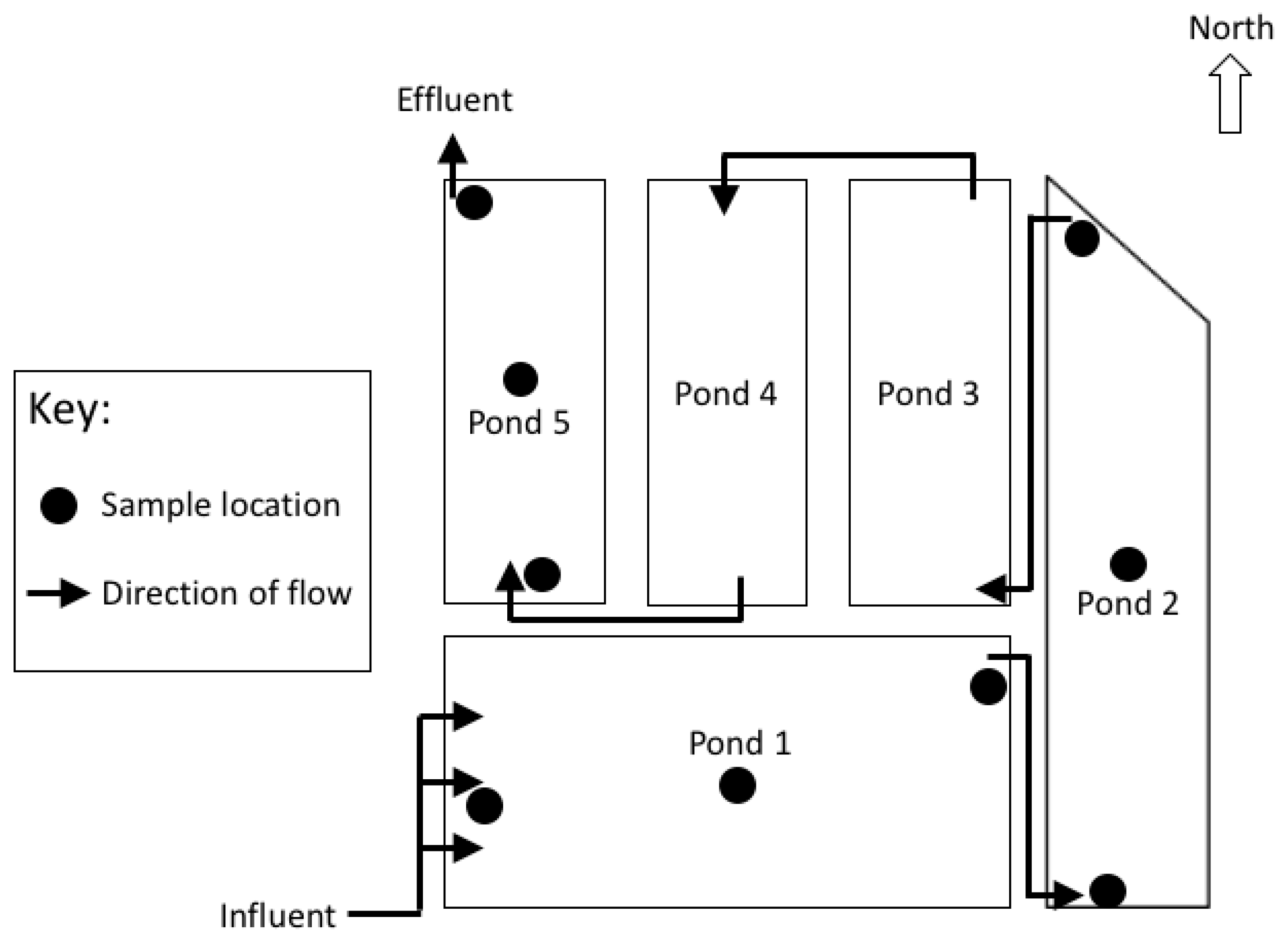
The Sanderson wastewater stabilization ponds (WSP) system comprises five ponds (Figure 1). Pond 1 is a 2.4 m deep facultative pond which receives raw influent. The remaining four ponds are shallow maturation ponds (Figure 1). Wastewater entering the Sanderson WSP is retained for an estimated 23 days before the treated effluent is released from the Pond 5 outlet. During the wet season (November to April, Southern Hemisphere), the system is expected to treat approximately 105 ML/day. In peak wet season (Summer, January to March) there is monsoonal rainfall (total rainfall ~1024 mm), high humidity, mean temperatures between 24.7–32 °C, and the highest wind speeds of the year (~134 km/hr) [19]. The WSPs are managed to cope with flooding and sewage dilution [4]. The dry season (May to October), is characterized by lower humidity and rainfall (total rainfall ~270 mm), warm, sunny days and cooler nights (mean temperatures between 21.6–31.8 °C). Both the low rainfall and high evaporation (~7.1 mm/d) [19] concentrate this WSP sewage.

2.2. Wastewater Collection

Wastewater samples (288) were collected in duplicate from ponds 1, 2 and 5 during the early wet (November and December) and dry (Winter, August and July) seasons in 2012 and 2013 (total of four occasions). In a pilot study using total bacterial fingerprinting (denaturing gradient gel electrophoresis), bacterial diversity was at its greatest in ponds 1, 2 and 5 (data not shown), so we focused on these ponds. At each site, surface and benthic water depths were sampled to target aerobes in the oxic top 10 cm of the water column and anaerobic bacteria in the bottom 10 cm from each pond’s inlet, middle and outlet. For each field campaign, samples were collected twice, once in the morning (6–10 am) and again in the afternoon (1–5 pm). In situ measurements of dissolved oxygen (DO), temperature and pH were collected during sampling using a HYDROLAB^® Quanta^® water quality instrument (Hydrolab Corporation^®, Austin, TX, USA).

2.3. Water Physicochemistry and Routine Fecal Indicator Bacteria (FIB) Culture Measurements

To determine if changes in standard water chemistry are associated with changes in microbial communities, we measured the same physicochemical variables that are routinely measured by the WSP operators. Wastewater samples of 1 L, 500 mL, 250 mL, 250 mL and 100 mL were collected for nutrients, biological oxygen demand (BOD), total organic carbon (TOC), total suspended solids (TSS)/total volatile solids (VSS), and alkalinity, respectively. One liter of water was also collected for bacterial community analysis. All samples were kept on ice during sampling. BOD was analyzed using the standard method 5210* [20] by the Water Chemistry Laboratory, Department of Primary Industry and Fisheries, Northern Territory (NT). TSS and VSS were measured and calculated according to ‘Standard Methods for the examination of water and wastewater’ [21]. Alkalinity was measured using an in-house Gran method with burette-titration (0.1 N Hydrochloric acid). Alkalinity species were determined using the USGS web-based alkalinity http://or.water.usgs.gov/alk/calculator. TOC analysis was according to the American Public Health Association method, APHA 5310B Total Organic Carbon [22] LabMark Pty Ltd. (Melbourne, VIC, Australia). Nutrient water chemistry was also analyzed by LabMark using unfiltered 1 L wastewater samples stored at −20 °C before analysis. Flow injection analysis (FIA) was used to determine ammonia, nitrate, nitrite and orthophosphate [23]. Prior to analysis, 15 mL of sample were filtered through polyethersulfone (PES), 0.45 µm Minisart^® high flow syringe filters (Sartorius Stedim, Biotech, Göttingen, Germany). For total Kjeldahl nitrogen (TN) and total phosphorus (TP), 10 mL of the remaining unfiltered sample was digested with alkaline potassium persulfate in the autoclave for 1 h at 121 °C, and also analyzed by FIA (Queensland Health Scientific Services, Coopers Plains, QLD, Australia).

E. coli and Enterococci were measured at the Pond 1 inlet and outlet, Pond 2 outlet and Pond 5 outlet by the Water Microbiology Laboratory (Dept. Primary Industry and Fisheries, Darwin, NT, Australia). E. coli were measured using Idexx Colilert AS4276.21-2005 and Enterococci were measured by Idexx Enterolert ASTM D6503-14 (2014) (IDEXX Laboratories Pty Ltd., Rydalmere, NSW, Australia). The detection limit for E. coli and Enterococci was one colony-forming unit (CFU) per 100 mL.

2.4. Bacterial Community Sequencing

To avoid clogging filter papers with algae, water samples (1 L) were left to settle overnight at 4 °C before filtering 100 mL through 0.45 µm filters (Pall Corporation, New York, NY, USA). DNA was extracted using the PowerWater DNA Isolation Kit (MoBio Laboratories, Carlsbad, CA, USA), following the manufacturer’s protocol.

Extracted DNA was sent to Molecular Research LP (MR DNA, Shallowater, TX, USA) for amplicon sequencing on the Illumina MiSeq platform targeting the V4V5 variable 16S rRNA region. Sequences were edited and classified using the MR DNA proprietary analysis pipeline (www.mrdnalab.com, Shallowater, TX, USA). Briefly, sequences were depleted of barcodes, and sequences were removed if < 200 bp (base pairs), or they had ambiguous base calls or homopolymer runs exceeding 6 bp. Remaining sequence data was denoized, chimeras and singleton sequences were removed and operational taxonomic units (OTUs) generated using clustering at 3% divergence or 97% similarity [24,25,26,27,28,29]. MR DNA then taxonomically classified the remaining OTUs with BLASTn against the curated GreenGenes database [30]. OTU sequence data (Table S1) and OTU metadata (Table S2) are available at Supplementaly Materials.

2.5. Statistical Analysis of Physicochemistry and Bacterial Community Sequences

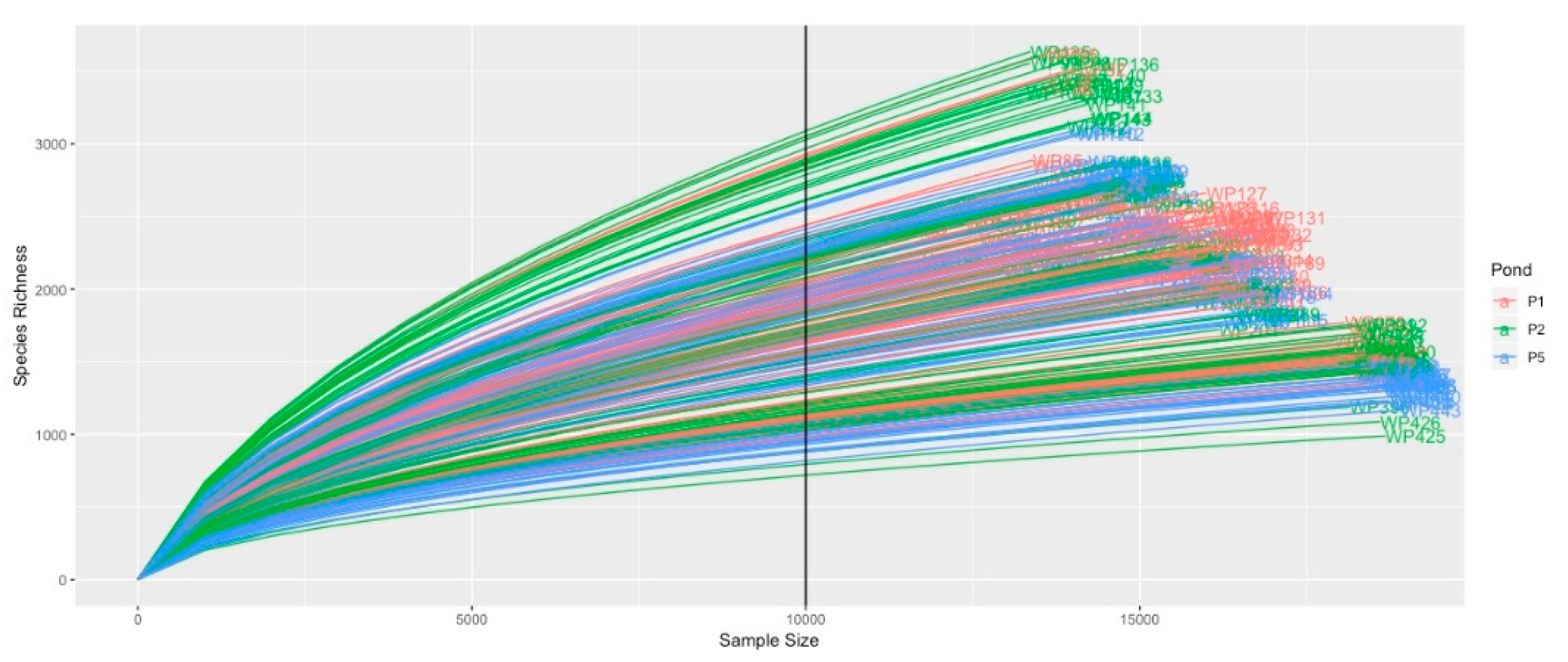
Subsequent filtering of sequences included comparing the sequence number between samples and excluding those with an outlying low sequence number (<10,532). However, initial filtering did not exclude any samples, because all were above the 10,000-sequence number threshold. OTUs found in only one sample were also excluded and data rarefied to 10,000 reads in phyloseq (Bioconductor, Bioconductor, Buffalo, NY). Before rarefying to 10,000 reads, each sample was assessed using rarefaction curves for potential loss of diversity (Figure A1 and Figure A2). Sequence data were square root transformed and a resemblance matrix was generated based on Bray-Curtis similarity. Physicochemical data were prepared for analysis by normalizing, removing co-linear variables (VSS, bicarbonate, PO₄⁺) and generating a resemblance matrix based on Euclidean distance.

Data were analyzed in R (version 1.1.423) using the packages phyloseq in Bioconductor [31] and IndVal [32]; in Primer-7 (Primer-E, Plymouth, UK), GenGIS version 2.4.1 [33], Stata-14 IC (STATA Corp, TX, USA), Cytoscape (version 3.4.0, www.cytoscape.org) and CoNet [34].

Differences in the bacteria between groups of samples were analyzed by permutational analysis of variance (PERMANOVA) with 9999 permutations. A cross design was used for the PERMANOVAs with six fixed factors: Year (2 levels), Season (2 levels), Pond (3 levels), Location (3 levels), Time (2 levels) and Depth (2 levels). A P value of < 0.05 (two-sided) was considered significant. For multiple comparisons, the Bonferroni correction was applied to P-values to counteract the chance of incorrectly rejecting the null hypothesis. PermDISP (Primer-E Ltd., Plymouth, UK) was used to check for homogeneity of variance between groups. Significant differences between levels of factors were identified using non-parametric pairwise testing.

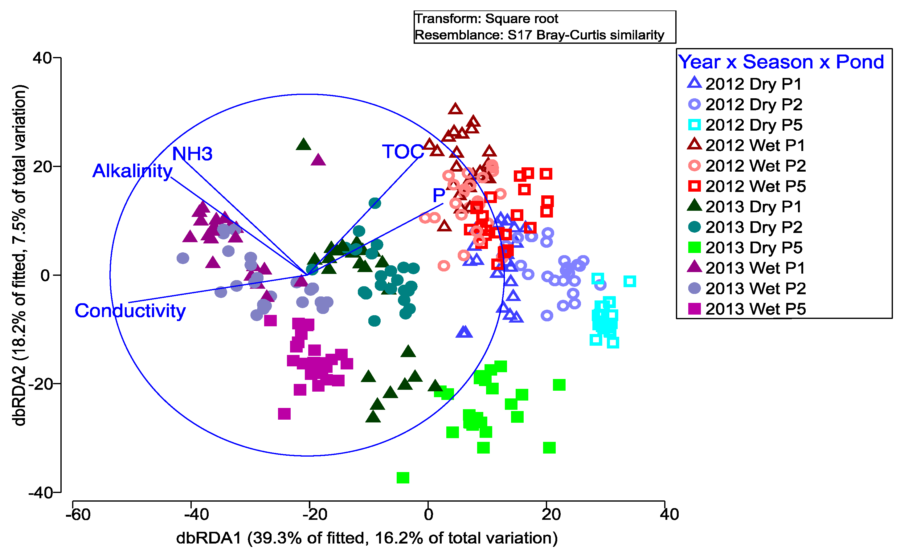
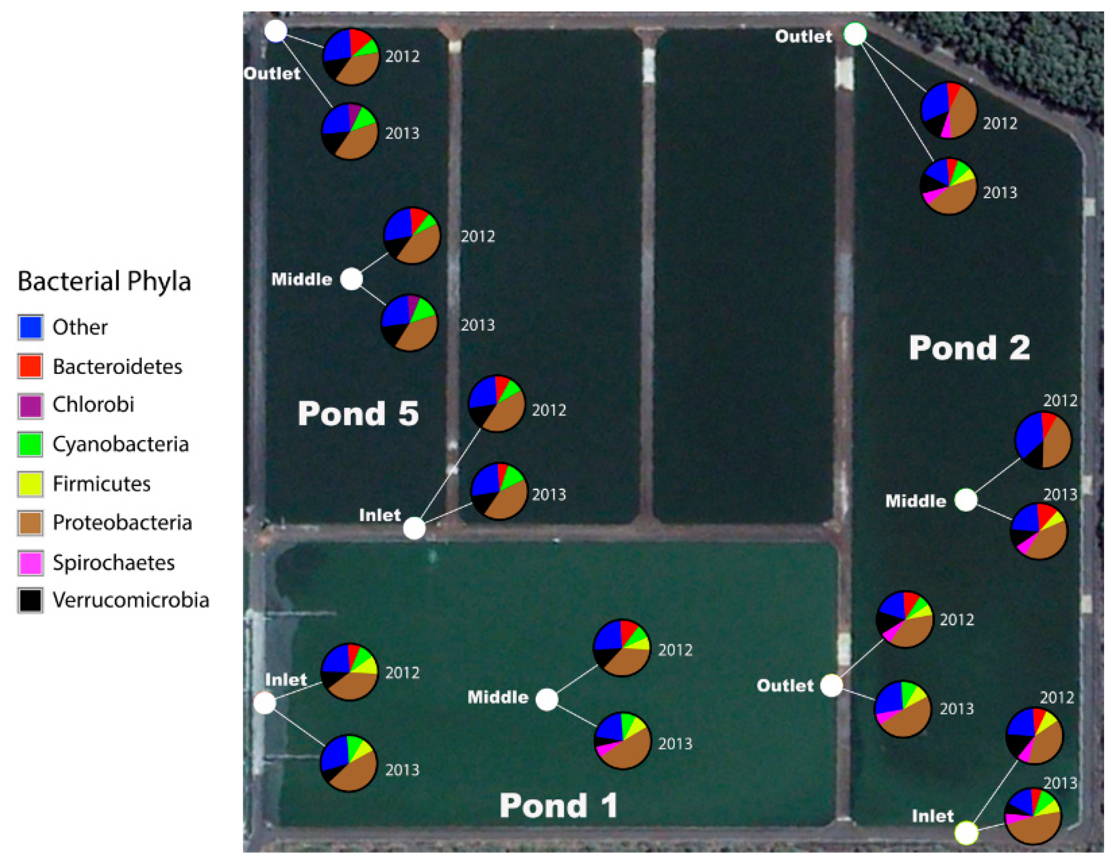
The relationship between the bacteria and physicochemical data was tested using a Distance-based Linear Model (DistLM) and distance-based redundancy analysis (dbRDA). Collinearity between physicochemical variables was checked, and VSS, bicarbonate and orthophosphate excluded from the analysis. Model selection for dbRDA was based on the lowest AIC and BEST elimination. Taxa sampled from each pond location in 2012–2013 were overlaid onto a georeferenced 2013 Google Earth© image using GenGIS. Differences between the phyla were analyzed by PERMANOVA using 9999 permutations and the same six fixed factor cross design described above (

Table A1. PERMANOVA analysis testing the differences in bacterial Phyla between year (2012, 2013), season (early wet and dry), pond number (P1, P2 and P5), location within the ponds (inlet, middle and outlet), time of day (6 am and 1 pm) and depth of the water sampled (surface and benthic). The term “df” indicates degrees of freedom, “ECV” square root of estimates of components of variation indicating the effect size as average% SV dissimilarity due to that factor (residual ECV 32.7). P value is based on >9978 unique permutations; “PermDISP” permutational distance-based test for homogeneity of multivariate dispersions for main factors. *** P value = 0.001; ** P value < 0.01; * P value < 0.05.

Factor PERMANOVA	Pseudo-F (df)	ECV	P Value	PermDISP P Value
Year	147.6 (1)	60.3	0.001 ***	0.001 ***
Season	48.2 (1)	19.4	0.001 ***	0.001 ***
Pond	82.4 (2)	50.2	0.001 ***	0.07
Location	5.2 (2)	2.6	0.001 ***	0.8
Time of day	8.7 (1)	3.2	0.001 ***	0.6
Depth	6.8 (1)	2.4	0.001 ***	0.7

). Key dominant WSP phyla were examined by calculating their family-level relative abundances with phyloseq and visualizing with ggplot2. Taxa patterns within the Firmicutes, Bacteroidetes and Cyanobacteria phyla were also examined by sub-setting each phyla with phyloseq and calculating the family-level relative abundances. We chose family-level analyses because the 16S region cannot accurately differentiate between closely-related species (Vêtrovský and Baldrian, 2013). For each phyla subset, the family-level change was assessed by PERMANOVA and the percent contribution of families were analyzed by Similarity Percentages (SIMPER) with a 50% contribution cut off (

Table A2. A. PERMANOVA analysis testing the differences in the Firmicutes phylum between year (2012, 2013), season (early wet and dry), pond number (P1, P2 and P5), location within the ponds (inlet, middle and outlet), time of day (6 am and 1 pm) and depth of the water sampled (surface and benthic). The term “df” refers to degrees of freedom, “ECV” square root of estimates of components of variation indicating the effect size as average% SV dissimilarity due to that factor (residual ECV 39.7). P value is based on >9804 unique permutations; “PermDISP” permutational distance-based test for homogeneity of multivariate dispersions for main factors. *** P value = 0.001; ** P value < 0.01; * P value < 0.05. B. Similarity percentages (SIMPER) analysis identifying species contributions to the change between ponds 1 and 5 for Firmicutes families: Thermoanaerobacteraceae, Lachnospiraceae, Clostridiaceae, Erysipelotrichaceae, Veillonellaceae, Bacillaceae, Ruminococcaceae, Peptococcaceae and Syntrophomonadaceae. Average dissimilarity between ponds 1 and 5 = 82.0%. Bray-Curtis similarity cut off = 50%.

(A)
Factor PERMANOVA	Pseudo-F (df)	ECV	P Value	PermDISP P Value
Year	47.1 (1)	22.4	0.001 ***	0.6
Season	37.3 (1)	19.9	0.001 ***	0.01 ***
Pond	30.7 (2)	22.1	0.001 ***	0.06
Location	3.3 (2)	6.1	0.001 ***	0.6
Time of day	1.6 (1)	2.6	0.01 **	0.3
Depth	1.3 (1)	1.9	0.05 *	0.1
(B)
Family	Pond 1 Average Abundance	Pond 5 Average Abundance	Family Contribution (%)	Cumulative Contribution (%)
Thermoanaerobacteraceae	1.7	3.9	2.0	2.0
Lachnospiraceae	3.9	2.0	1.6	3.6
Clostridiaceae	1.1	2.3	1.4	5.0
Erysipelotrichaceae	1.2	2.0	1.3	8.8
Veillonellaceae	1.6	0.1	1.1	13.4
Bacillaceae	0.7	1.6	1.0	14.4
Ruminococcaceae	1.4	0.2	0.9	17.2
Peptococcaceae	0.1	1.1	0.8	18.9
Syntrophomonadaceae	0.2	1.0	0.7	23.6

,

Table A3. A. PERMANOVA analysis testing the differences in the Bacteroidetes phylum between year (2012, 2013), season (early wet and dry), pond number (P1, P2 and P5), location within the ponds (inlet, middle and outlet), time of day (6 am and 1 pm) and depth of the water sampled (surface and benthic). The term “df” represents degrees of freedom, “ECV” square root of estimates of components of variation indicating the effect size as average% SV dissimilarity due to that factor (residual ECV 36.0). P value is based on >9912 unique permutations; “PermDISP” permutational distance-based test for homogeneity of multivariate dispersions for main factors. *** P value = 0.001; ** P value < 0.01; * P value < 0.05. B. Similarity percentages (SIMPER) analysis identifying species contributions to the change between ponds 1 and 5 for Bacteroidetes indicator families: Chitinophagaceae, Porphyromonadaceae, Cytophagaceae and Cryomorphaceae. Average dissimilarity between ponds 1 and 5 = 79.5%. Bray-Curtis similarity cut off = 50%.

(A)
Factor PERMANOVA	Pseudo-F (df)	ECV	P Value	PermDISP P Value
Year	85.2 (1)	27.6	0.001 ***	0.001 ***
Season	70.9 (1)	25.1	0.001 ***	0.3
Pond	28.2 (2)	19.2	0.001 ***	0.001 ***
Location	2.6 (2)	4.7	0.001 ***	0.6
Time of day	2.0 (1)	3.0	0.001 ***	0.4
Depth	1.9 (1)	2.8	0.001 ***	0.7
(B)
Family	Pond 1 Average Abundance	Pond 5 Average Abundance	Family Contribution (%)	Cumulative Contribution (%)
Chitinophagaceae	3.7	0.8	2.0	2.0
Porphyromonadaceae	2.7	0.5	1.5	5.0
Cytophagaceae	1.7	0.8	1.0	13.0
Cryomorphaceae	0.2	0.8	0.8	38.8

and

Table A4. A. PERMANOVA analysis testing the differences in the Cyanobacteria phylum between year (2012, 2013), season (early wet and dry), pond number (P1, P2 and P5), location within the ponds (inlet, middle and outlet), time of day (6 am and 1 pm) and depth of the water sampled (surface and benthic). The term “df” means degrees of freedom, “ECV” square root of estimates of components of variation indicating the effect size as average% SV dissimilarity due to that factor (residual ECV 39.7). P value is based on >9912 unique permutations; “PermDISP” permutational distance-based test for homogeneity of multivariate dispersions for main factors. *** P value = 0.001; ** P value < 0.01; * P value < 0.05. B. Similarity percentages (SIMPER) analysis identifying species contributions to the change between ponds 1 and 5 for Cyanobacteria families: Synechococcaceae and Phormidiaceae. Average dissimilarity between ponds 1 and 5 = 19.4%. Bray-Curtis similarity cut off = 50%.

(A)
Factor PERMANOVA	Pseudo-F (df)	ECV	P Value	PermDISP P Value
Year	47.1 (1)	22.4	0.001 ***	0.6
Season	37.3 (1)	19.9	0.001 ***	0.01 **
Pond	30.7 (2)	22.1	0.001 ***	0.1
Location	3.3 (2)	6.1	0.001 ***	0.6
Time of day	1.6 (1)	2.6	0.01 **	0.2
Depth	1.3 (1)	1.9	0.04 *	0.1
(B)
Family	Pond 1 Average Abundance	Pond 5 Average Abundance	Family Contribution (%)	Cumulative Contribution (%)
Synechococcaceae	0.8	0.7	16.0	16.0
Phormidiaceae	0.4	0.5	15.6	31.5

). Indicator bacteria were defined as those taxa that were present in 100% of samples (n = 96) from a particular pond. IndVal [32] was used to identify indicator taxa, and Cytoscape was used to show their relative abundance across the different ponds. Because these indicator bacteria are not currently used for WSP monitoring, we refer to them as ‘new’ or ‘indicator candidates’, because they are not yet validated. 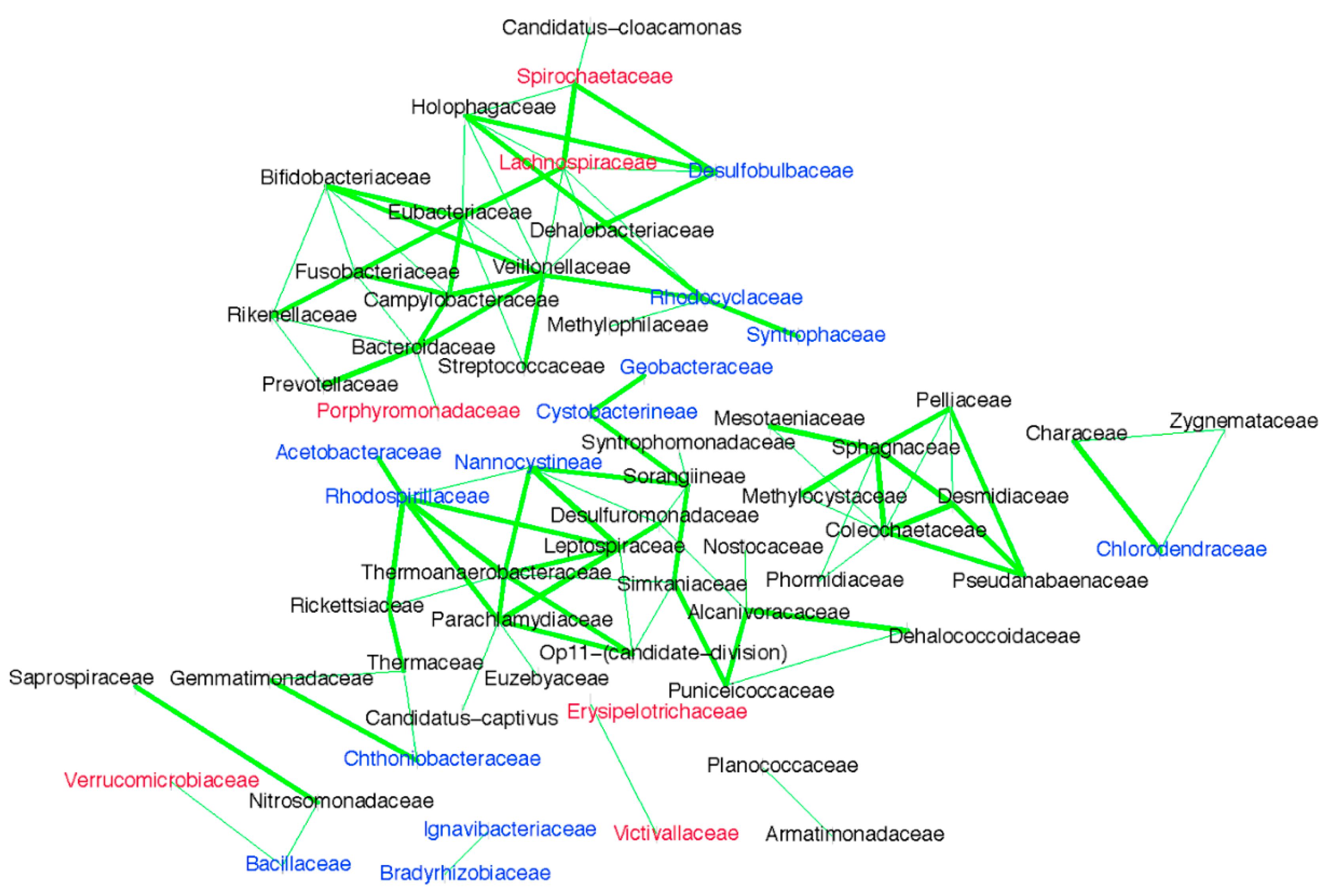The core microbiome was taken to be taxa present in 90% of all samples [35] to distinguish between bacteria that were consistently found in wastewater (hereafter referred to as the ‘core microbiome’) with bacteria that are transient and opportunistic [35,36,37,38].The co-occurrence of core bacteria was determined by CoNet analysis [34]. To calculate co-occurrence, we set a minimum of 20% occurrences among replicates and transformed (log-2) the data values. An automatic threshold was used to include only the top and bottom 100 edges. Kendall rank correlations (threshold = 0.05) were calculated after generating a Bray Curtis distance matrix (threshold = 0.05), and we tested the strength of the correlations between taxa with Fisher’s Z-test, while accounting for multiple testing using Bonferroni to include only those taxa that significantly (P < 0.05) co-occurred.

3. Results

3.1. Comparing Whole Bacterial Community Changes in Ponds 1, 2 and 5

Bacterial composition in the WSP changed over years, wet and dry seasons and between ponds 1, 2 and 5 (Figure 2). Of the factors measured, the year had the greatest influence on bacterial composition (

Table 1. Permutational analysis of variance (PERMANOVA) analysis, testing the differences in taxa between year (2012, 2013), season (early wet and dry), pond number (P1, P2 and P5), location within the ponds (inlet, middle and outlet), time of day (6 am and 1 pm) and depth of the water sampled (surface and benthic). The designation “df” refers to degrees of freedom, “ECV” to the square root of estimates of components of variation indicating the effect size as average% SV dissimilarity due to that factor (residual ECV 32.7). The P value is based on >9700 unique permutations; “PermDISP” permutational distance-based test for homogeneity of multivariate dispersions for main factors. *** P value = 0.001; ** P value < 0.01; * P value < 0.05.

Factor PERMANOVA	Pseudo-F (df)	ECV	P Value	PermDISP P Value
Year	84.1 (1)	24.9	0.001 ***	0.02 *
Season	57.6 (1)	20.5	0.001 ***	0.1
Pond	28.4 (2)	17.5	0.001 ***	0.001 ***
Location	2.6 (2)	4.2	0.001 ***	0.5
Time of day	2.4 (1)	3.2	0.001 ***	1.0
Depth	1.9 (1)	2.6	0.006 **	0.5
Year × Season	39.3 (1)	23.9	0.001 ***	0.001 ***
Year × Pond	8 (2)	12.5	0.001 ***	0.001 ***
Year × Location	2.1 (2)	4.9	0.001 ***	0.006 **
Year × Season × Pond	5.5 (2)	14.2	0.001 ***	0.001 ***
Year × Pond × Location	2.5 (4)	10.1	0.001 ***	0.001 ***
Year × Season × Pond × Time	3.9 (2)	16.0	0.001 ***	0.001 ***

). On average, only 27.7% of the OTUs detected in 2012 were also found in 2013. Bacteria also loosely grouped by season and pond number (Figure 2), with distinct communities between ponds 1, 2 and 5 in 2013 (

Table 2. Summary details for measured physicochemical variables and standard cultured fecal indicator bacteria (FIB) (averages and standard deviations (SDs)) for 2012 and 2013, the wet and dry season, and ponds 1, 2 and 5. A. Average wastewater stabilization ponds (WSP) physicochemical and FIB levels according to year, season and pond number. B. Average E. coli and Enterococci colony counts between the Pond 1 inlet and the Pond 5 outlet for 2012 and 2013 and the wet and dry seasons. n = sample number, SD = standard deviation, mg/L = milligrams per liter, S/m = siemens per meter, BOD = biological oxygen demand, TOC = total organic carbon, TSS = total suspended solids, VSS = total volatile solids, NH₃ = ammonia, NO₃ = nitrate, NO₃ nitrite, TN = nitrogen, PO₄ = orthophosphate, TP = total phosphorus, CFU = colony forming units.

(A)
Variable	2012 (n= 144)	2013 (n= 144)	Dry Season (n = 144)		Wet Season (n = 144)	Pond 1 (n = 96)	Pond 2 (n = 96)	Pond 5 (n = 96)
	Mean ± SD	Mean ± SD	Mean ± SD		Mean ± SD	Mean ± SD	Mean ± SD	Mean ± SD
DO (mg/L)	5.6 ± 5.9	5.1 ± 5.6	6.5 ± 6.1		4.1 ± 5.1	5.2 ± 5.3	4.5 ± 5.1	6.4 ± 6.6
Conductivity (S/m)	540.0 ± 44.5	670.3 ± 81.1	553.0 ± 54.9		657.4 ± 92.8	611.9 ± 86.1	604.3 ± 91.4	599.3 ± 99.6
Temperature (oC)	31.6 ± 2.9	28.0 ± 4.7	26.9 ± 3.8		32.7 ± 2.2	30.1 ± 4.0	29.9 ± 4.0	29.3 ± 4.7
pH	7.8 ± 0.8	7.6 ± 0.6	7.7 ± 0.8		7.8 ± 0.6	7.4 ± 0.6	7.6 ± 0.6	8.2 ± 0.8
TSS (mg/L)	207.9 ± 35.4	154.4 ± 36.6	203.0 ± 42.4		159.3 ± 35.8	196.9 ± 47.3	184.8 ± 39.0	161.8 ± 41.0
VSS (mg/L)	191.5 ± 29.5	148.0 ± 27.7	182.5 ± 39.1		156.9 ± 27.2	183.3 ± 36.9	171.0 ± 31.7	154.9 ± 33.6
BOD (mg/L)	121.2 ± 38.4	73.0 ± 20.0	111.6 ± 48.0		82.7 ± 17.8	104.3 ± 41.8	98.8 ± 45.5	88.2 ± 25.3
TOC (mg/L)	92.0 ± 11.7	62.0 ± 20.3	81.0 ± 17.9		73.0 ± 25.4	79.8 ± 20.2	82.0 ± 21.0	69.3 ± 23.6
Alkalinity (mg/L)	130.7 ± 24.4	144.8 ± 20.7	126.0 ± 23.3		149.5 ± 17.4	152.5 ± 18.4	139.8 ± 19.5	121.0 ± 21.6
Carbonate (mg/L)	0.2 ± 0.1	0.3 ± 0.2	0.3 ± 0.3		0.2 ± 0.1	0.2 ± 0.1	0.2 ± 0.2	0.3 ± 0.3
Bicarbonate (mg/L)	159.1 ± 29.6	175.4 ± 26.0	153.2 ± 28.3		181.4 ± 22.0	185.5 ± 22.5	169.4 ± 24.1	146.9 ± 26.4
NH3 (mg/L)	17.2 ± 5.3	19.4 ± 6.5	16.0 ± 6.7		20.7 ± 4.2	22.5 ± 4.8	20.2 ± 3.1	12.3 ± 4.5
NO2 (mg/L)	0.0 ± 0.0	0.5 ± 0.7	0.4 ± 0.8		0.1 ± 0.1	0.2 ± 0.3	0.1 ± 0.2	0.5 ± 0.9
NO3 (mg/L)	0.0 ± 0.0	0.2 ± 0.2	0.1 ± 0.2		0.1 ± 0.1	0.1 ± 0.1	0.1 ± 0.1	0.2 ± 0.2
TN (mg/L)	34.8 ± 4.9	36.8 ± 13.8	37.2 ± 13.6		34.4 ± 5.4	40.5 ± 14.7	37.3 ± 5.5	29.7 ± 4.4
PO4 (mg/L)	4.8 ± 0.6	1.6 ± 0.8	3.4 ± 2.0		3.0 ± 1.4	3.0 ± 1.9	3.1 ± 1.7	3.6 ± 1.6
TP (mg/L)	6.9 ± 0.7	4.1 ± 0.5	5.6 ± 2.0		5.4 ± 1.0	5.5 ± 1.5	5.4 ± 1.5	5.5 ± 1.7
E. coli (Log CFU /mL)	6.57 ± 6.78	6.59 ± 6.80	6.52 ± 6.72		6.63 ± 6.84	6.88 ± 6.83	5.19 ± 4.93	3.25 ± 3.18
Enterococci (Log CFU /mL)	5.37 ± 5.60	5.62 ± 5.75	5.42 ± 5.65		5.57 ± 5.72	5.75 ± 5.71	3.46 ± 3.48	2.94 ± 2.63
(B)
FIB	2012 (n = 16)		2013 (n = 16)		Dry Season (n = 16)		Wet Season (n = 16)
	Pond 1 Inlet	Pond 5 Outlet	Pond 1 Inlet	Pond 5 Outlet	Pond 1 Inlet	Pond 5 Outlet	Pond 1 Inlet	Pond 5 Outlet
	Mean ± SD	Mean ± SD	Mean ± SD	Mean ± SD	Mean ± SD	Mean ± SD	Mean ± SD	Mean ± SD
E. coli (Log CFU /mL)	7.12 ± 6.57	3.35 ± 3.34	7.15 ± 6.58	3.12 ± 2.57	7.08 ± 6.41	3.07 ± 2.57	7.19 ± 6.58	3.38 ± 3.31
Enterococci (Log CFU /mL)	5.96 ± 4.66	2.93 ± 2.15	6.00 ± 5.66	2.96 ± 2.96	5.99 ± 5.32	2.92 ± 2.73	5.96 ± 5.61	2.97 ± 2.16

and Figure 2). Differences in the pond-bacterial community was also greatest between the first (Pond 1) and last pond (Pond 5) with 29.2% of OTUs the same between these ponds. Small, yet statistically significant (p < 0.01), changes to the bacterial community were also measured between the morning and afternoon, and between the surface and benthic water samples (Table 1).

3.2. Physicochemical Variables, the Bacterial Community and FIB

Patterns in the wastewater bacterial community composition were most correlated with conductivity, TOC and phosphorus (P) (Figure 3). The first two axes of the dbRDA with standard water chemistry explained 23.7% of the bacterial community change (Figure 3). Conductivity was the greatest physicochemical driver correlating with large bacterial community change between 2012 and 2013 (Figure 3). In 2012 the wastewater conductivity was lower than in 2013 (Table 2 and Figure 3). In 2013, conductivity was also higher in the wet compared to the dry season (Table 2 and Figure 3). TOC and P had an inverse relationship with conductivity, with the highest average TOC and P concentrations measured for 2012 and the lowest for 2013 (Table 2A and Figure 3). Bacteria composition changed between ponds 1, 2 and 5 along an alkalinity and NH3 gradient, with highest average alkalinity and NH3 concentrations measured in the Pond 1 wastewater and the lowest in Pond 5 (Table 2 and Figure 3). E. coli and Enterococci concentrations decreased between ponds (Table 2). The 99.99% E. coli and 99.9% Enterococci removal did not change throughout the study (Table 2B).

3.3. Bacterial Taxa that Characterize Ponds 1, 2 and 5

The abundance of several bacterial phyla changed across the ponds and between the years 2012–2013 (Table A1 and Figure 4). The Proteobacteria were dominant in all samples. However, E. coli (Family: Enterobacteriaceae), which belong to the Proteobacteria phylum, were not detected. Another dominant phylum was the Firmicutes. The abundance of this phylum decreased from 11.1% (2012) and 8.4% (2013) in Pond 1 to below 6% of the sampled population in Pond 5 (Figure 4). In contrast, in 2012 the Bacteroidetes phylum was abundant in all ponds and contributed to 7.3–14.7% of bacteria measured in each sample, regardless of location. However, in 2013, the abundance of Bacteroidetes often decreased below 6% at each sampled site, and were only dominant at the Pond 2 inlet (6.2%), middle (12.7%) and outlet (6.4%), and the Pond 5 inlet (6.2%) (Figure 4). With the exception of Pond 2 in 2012, regardless of the sample location, Cyanobacteria contributed to greater than 6% of the total population, even at the Pond 1 inlet. The Phyla known as Chlorobi, Spirochaetes and Verrucomicrobia formed a small portion of the dominant bacteria (Figure 4).

3.4. Potential Pond-Indicators and Gut vs. Environmental Bacteria

Indicator bacteria were defined as those taxa that were present in 100% of samples (n = 96) from a particular pond. Forty-eight bacterial families were tested using Indicator Value (IndVal, [32]) to find indicator candidates specific for ponds 1, 2 or 5. The Enterococcaceae was not selected because they were only measured in 11 of 288 samples. Bacterial indicators for pond 1 were gut-associated such as Clostridiaceae, Ruminococcaceae, Lachnospiraceae, Porphyromonadaceae, Erysipelotrichaceae, Pseudomonadaceae and Victivallaceae (Figure 5). In contrast, indicators for Pond 5 were environmental bacteria, including Geobacteraceae, Synechococcaceae (ponds 1 and 5), Solibacteraceae (ponds 1, 2 and 5), Hyphomicrobiaceae (ponds 2 and 5), Oxalobacteraceae (Pond 5) and Planctomycetaceae (Pond 5).

3.5. Detailed Analysis of Selected Phyla

The phyla Firmicutes, Bacteroidetes and Cyanobacteria were selected for more detailed analysis because they were dominant (Figure 4) and contained potential indicators like Bacillaceae, Lachnospiraceae, Chitinophagaceae and Synechococcaceae, for different ponds (Figure 5).

3.5.1. Firmicutes

Thirty-nine Firmicutes families were detected (Supplementary Figure S1), and of these only fifteen had a relative abundance ≥ 0.1% (Figure 6). Lachnospiraceae was dominant across the ponds, and five families were indicators for specific ponds (Figure 6). Ruminococcaceae, Veillonellaceae and Lachnospiraceae relative abundance declined from ponds 1 to 5 (Figure 6). Families that increased in abundance included: Peptococcaceae, Syntrophomonadaceae, Thermoanaerobacteraceae, Clostridiaceae and Bacillaceae (Figure 6). Some Firmicutes families like Erysipelotrichaceae were indicators for multiple ponds (Figure 5 and Figure 6).

3.5.2. Bacteroidetes

Sixteen Bacteroidetes families were identified in pond samples. Families with environmental roles were abundant and increased between ponds 1 and 5 (Figure 7). For example, the most common family, Chitinophagaceae, increased between Pond 1 and Pond 5 (Figure 7). However, gut-associated families like Porphyromonadaceae and Cytophagaceae declined between ponds 1 and 5. Four Bacteroidetes families were indicators for Sanderson wastewater ponds: Porphyromonadaceae (Pond 1); Cytophagaceae (ponds 1 and 2); Cryomorphaceae (Pond 2); and Chitinophagaceae (Figure 7).

3.5.3. Cyanobacteria

Of the nine Cyanobacteria families identified, two were dominant, Phormidiaceae and Synechococcaceae (Figure 8). Phormidiaceae increased from Pond 1 to Pond 5, but Synechococcaceae decreased (Figure 8). The Synechococcaceae was an indicator for all ponds and had the highest relative abundance in the Pond 1 samples (Figure 8).

3.6. The WSP Sewage Core Microbiome

Regardless of sample timing and location, 282 bacterial families were present in at least 90% of the samples collected between 2012 and 2013. This core microbiome of wastewater included all 48 indicator–bacteria families. CoNet analysis was used to identify 63 core families that significantly correlated (p < 0.05) with at least one other family, including 19 of the 48 indicator families (Figure 9). Indicator taxa generally co-occurred together in small groups of two or three, with only three of those taxa (Chthoniocacteraceae, Chlorodendraceae and Porphyromonadaceae) not significantly correlated with other pond indicators (Figure 9).

4. Discussion

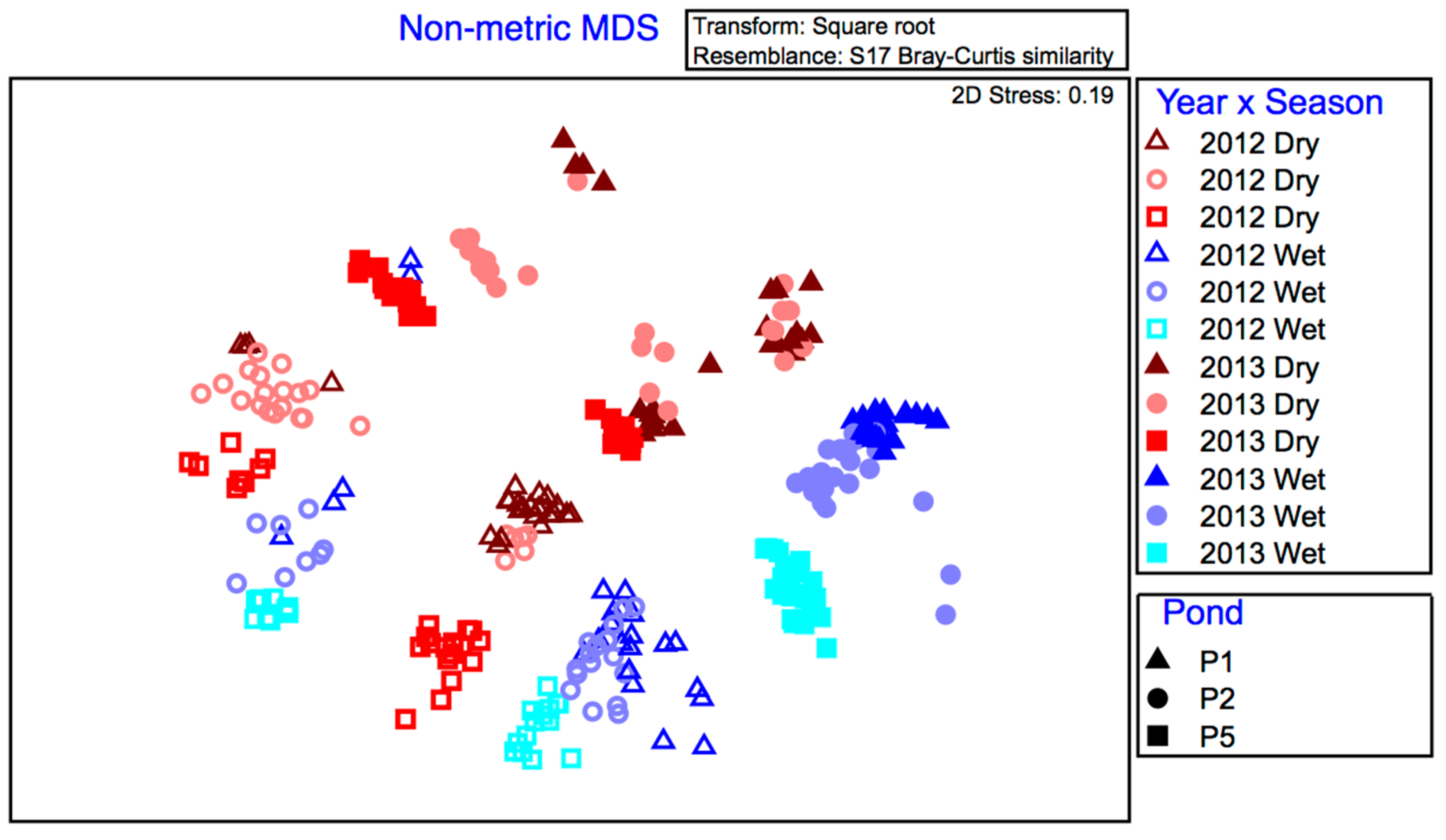
The bacterial communities in wastewater stabilization ponds (WSPs) at Sanderson were dynamic over space (ponds) and time (season and years). Other wastewater treatment pond studies suggest that the composition of fecal and non-fecal bacteria can change between wastewater systems, and are likely responding to different climatic conditions [8,11,39,40,41]. A two-year study of an anaerobic bioreactor also showed that the bacterial composition changed every few months [42]. Because wastewater systems and ponds can have dynamic bacterial populations, we recommend pond managers collect regular samples over several years to develop a comprehensive baseline of bacterial communities.

We measured standard WSP physicochemical variables and found that conductivity explained 14% of the bacterial change. However, over 76% of the bacterial change was not explained by the physicochemical variables measured, suggesting that other unmeasured variables likely influenced the pond bacteria. There is conflicting information on the physical and chemical drivers of bacterial population change [16], although it is generally accepted that diverse bacterial communities are likely to consist of a vast array of different ecological niches and nutritional pathways [11,41].

Consequently, it is not surprising that the overall influence of a single variable like TOC is not consistent over time or between studies. Previous studies have also concluded that unmeasured variables are likely involved in bacterial community change [4,17,18]. Potentially important factors that have not been included in analyses of the bacterial communities at Sanderson include sewage inflow and specific weather variables. A previous Sanderson diel study showed that the water chemistry changed according to the rate of raw sewage inflow [18]. Similarly, Shanks et al. [8] also found inflow affected the bacterial composition because the bacteria that line sewer pipes seed wastewater ponds. Weather variables (e.g., wind direction and speed, cloud cover, irradiance and rainfall) could explain the distinct Sanderson bacterial communities measured in 2013 after the second driest wet season on record [19]. To fully understand and predict the dynamic bacterial change in wastewater systems, it may be necessary to expand the variables measured to include wind parameters, inflow rates, rainfall and solar radiation.

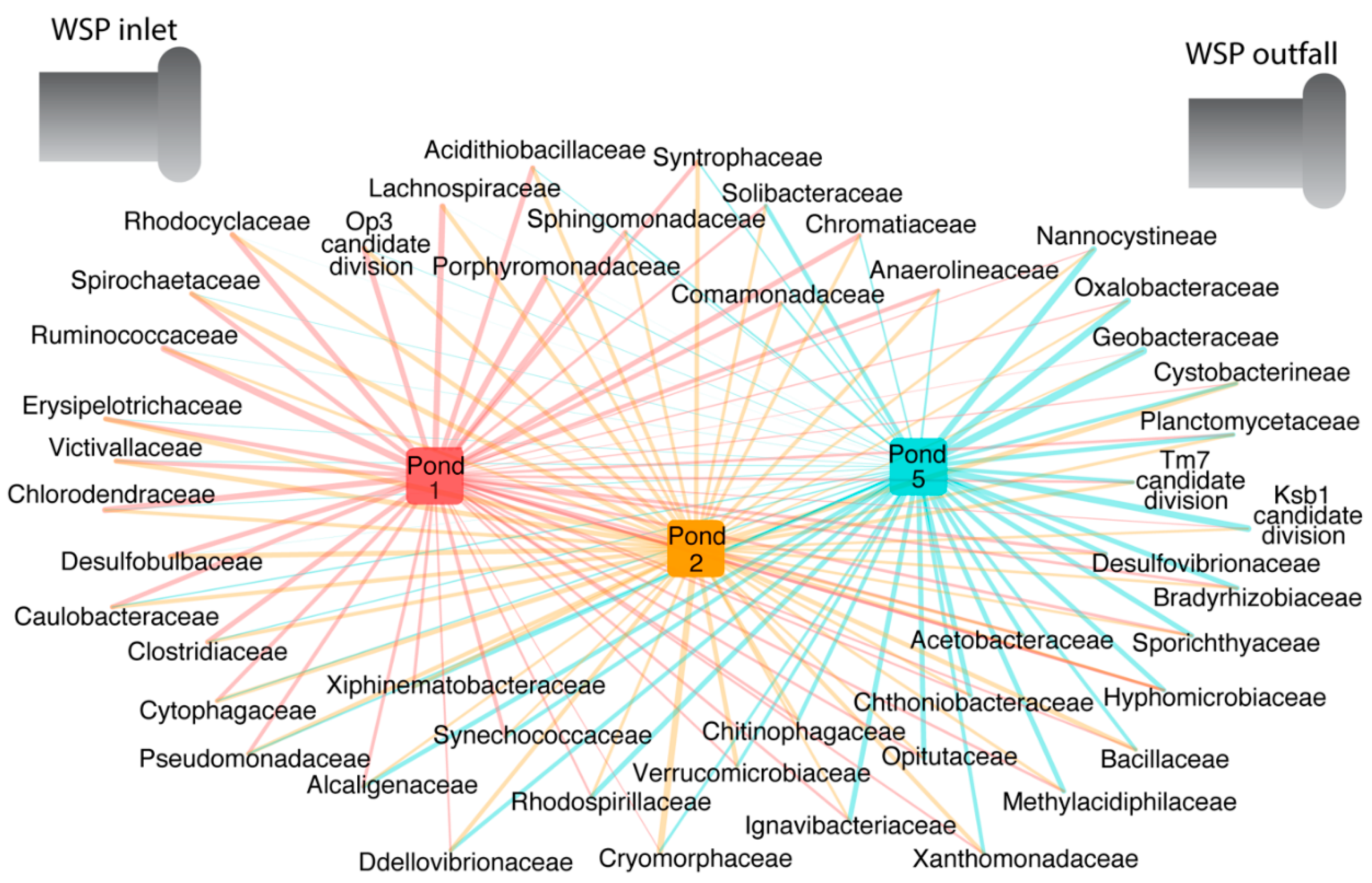
When the bacterial community in the raw influent and ‘treated’ effluent are not significantly different, this is taken as an indication that sanitation in a WSP has failed [1]. In contrast then, if ponds are functioning and effecting sanitation, it ought to be possible to show this through a measurable difference in the bacterial communities in the influent compared to the treated effluent. Using 16S rRNA gene sequencing, we identified new pond-indicator bacteria that represent each treatment pond and can complement current standard FIB. For the measured facultative and maturation ponds, new pond-indicators were identified using IndVal. Indicators for each pond were defined as those taxa that were present in 100% of the samples from a target pond (Figure 4). Many of the indicators of the facultative (Pond 1) and first maturation pond (Pond 2) are common in the human gut, such as Clostridiaceae, Ruminococcaceae and Lachnospiraceae [16,43]. These bacterial groups were also detected in other sewage studies [8,11,41]. However, non-fecal bacteria were also detected in the first pond and were a conspicuous component of the sewage microbiome (Figure 5 and Figure 8). 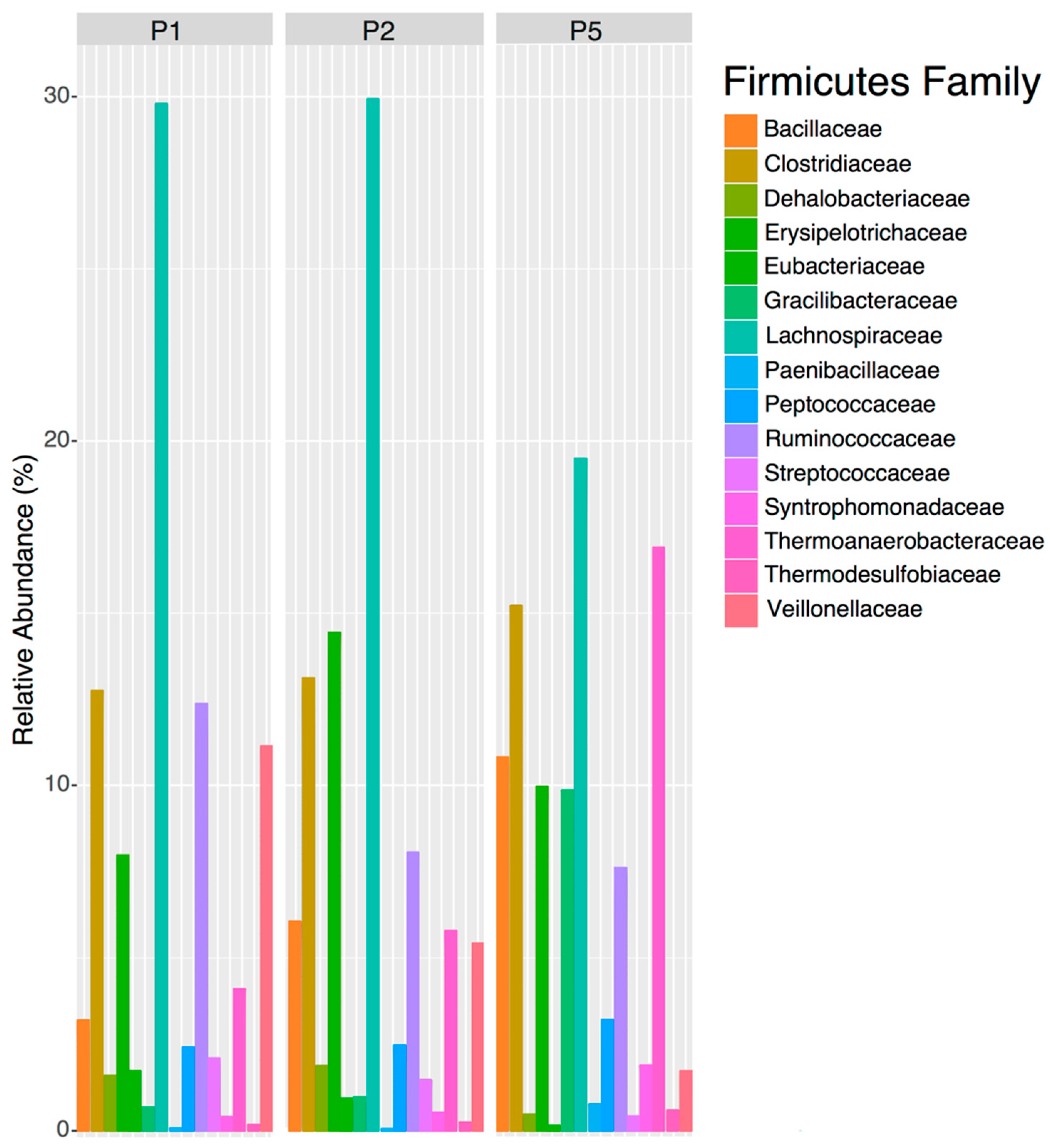The co-presence of dominant non-fecal bacteria was also reported in other studies, presumably because the influent is a mix of gray water, effluent and pipe biofilms, all of which enter the waste stabilization ponds, mixing both human-associated bacteria with those found in the environment [8,44]. By the final maturation pond (Pond 5) the human-gut bacteria from the first two ponds were largely replaced by bacteria that are typically found in the environment and contribute to ecosystem function, like nitrogen cycling. This pattern suggests that the Sanderson ponds are removing the human-gut bacteria, and that nitrogen removal is highest after Pond 1. Thus, the succession pattern of the new pond-indicators, in which human-gut bacteria in ponds 1 and 2 are supplanted by environmental bacteria in Pond 5, suggests that the Sanderson ponds are performing their expected function. These results suggest that future indicators of human-fecal pollution should target Firmicutes families like Ruminococcaceae, Spirochaetaceae and Clostridiaceae.

In addition to identifying new candidates for pond-indicator bacteria, whole-community analysis of the WSP has shed light on the previous microbiological ‘black box’ for these ponds and challenged some of the previous assumptions about non-fecal bacteria and Cyanobacteria. We found that non-fecal bacteria dominated the core wastewater microbiome for Sanderson. 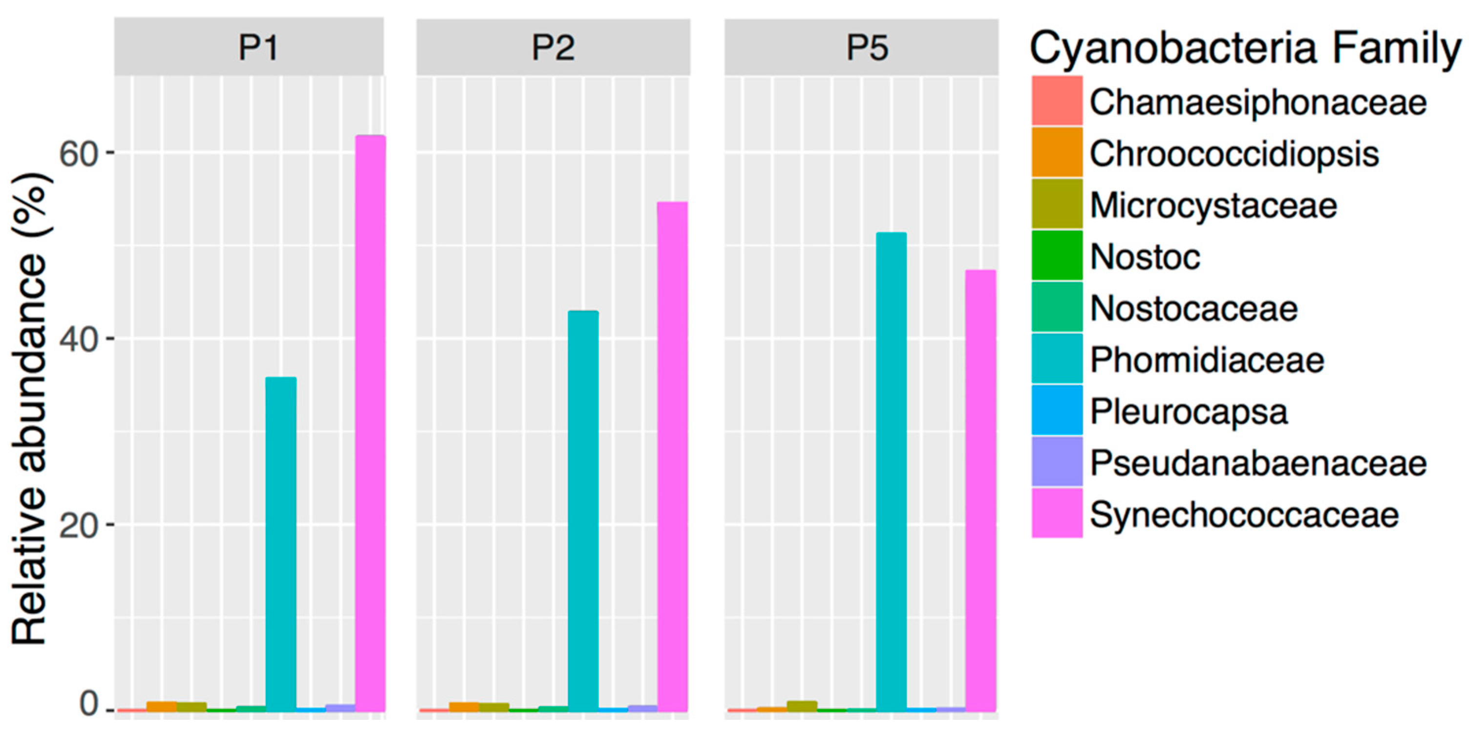This result is similar to other wastewater studies that found 80–90% of bacteria are non-fecal [8,11,45]. Cyanobacteria represented greater than 6% of the WSP bacterial population regardless of sample timing and location, which was primarily due to the high relative abundance of the families Synechococcaceae and Phormidiaceae. Within the wastewater industry, it is assumed that Cyanobacteria become problematic in maturation ponds due to the warm, calm and low organic loading/nutrient conditions [4,46]. Consequently, pond managers have considered replacing these ponds with an aerated rock filter to reduce retention time, ammonia levels and Cyanobacteria [4]. Contrary to expectations of pond managers, Cyanobacteria were abundant at the Pond 1 inlet, suggesting that they may be entering the WSP in the influent. Thus, whole community analysis is a useful tool for identifying the resident bacteria in a WSP and testing assumptions about key taxa before implementing management strategies.

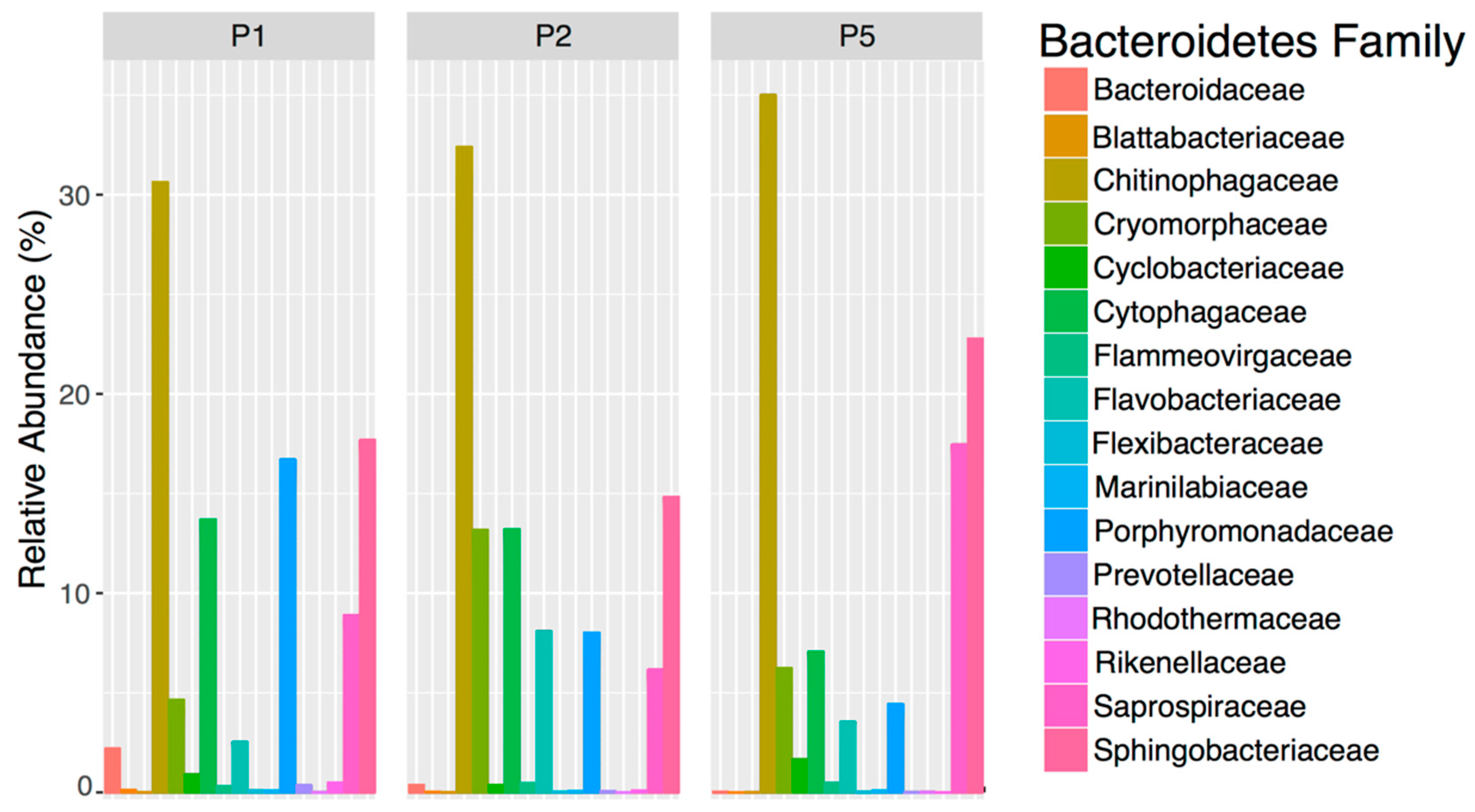
It is imperative to consider the taxonomic classification level when identifying indicators for a bacterial population, because bacteria with the same high-level taxonomic classification can have different ecological roles. For example, we found that Bacteroidetes (phylum) did not decline from ponds 1–5. The continued persistence of Bacteroidetes across the ponds was unexpected because, although a diverse bacterial phylum, they are considered representative of fecal bacteria [4,46]. However, a more in-depth investigation of Bacteroidetes at the family level revealed that fecal groups like Bacteroidaceae did, in fact, decline between ponds 1–5 and that their persistence at the phylum level was likely due to the increase in those families that typically occur in the environment like Chitinophagaceae [47]. Currently, there is no consensus for which bacterial taxonomic level to use when classifying indicators, with some studies on wastewater treatment using multiple levels, while others use the family level [8,11,44,48]. Therefore, to avoid including taxa that may complicate spatial and temporal patterns, we recommend choosing the lowest possible taxonomic level for pond indicators.

In this study, E. coli sequences were not detected, and Enterococci sequences were detected in less than 4% of samples, but we note that E. coli and Enterococci were cultured from these ponds. E. coli were not resolved by 16S rRNA sequencing because the short sequence length was not sufficient for taxonomic resolution of this genus [49,50]. It is also possible that the DNA extraction method from a highly complex wastewater matrix and diverse microbial population results in different lysis efficiencies for different bacterial groups, and may not have been suitable for gram positive Enterococci [51,52,53]. There are several other possible explanations: Preferential primer binding during DNA amplification to other bacterial DNA present [54] or the abundance of these bacteria in samples was rare compared to other taxa and their DNA was not amplified to detectable levels [53]. Regardless, 16S rRNA sequencing was intended to supplement routine FIB monitoring, and not be utilized as a replacement.

In addition to the current monitoring practices, managers could apply our new pond-indicator candidates, which are a combination of human-gut and environmental bacteria. Because most Sanderson pond-indicators co-occur, it is possible to select a single family in each group as a representative. For example, the pond 1 and 2-indicator family Spirochaetaceae could act as a surrogate for Lachnospiraceae and Desulfobulbaceae because they co-occur in Sanderson wastewater. In future, combining our new pond-indicators with the standard fecal indicator bacteria will lead to a robust monitoring approach that is not only locally relevant, but also provides a bespoke tool-box with indicator candidates for tropical environments worldwide.

5. Conclusions

Using 16S rRNA gene sequencing, we identified a combination of human-gut and environmental bacteria specific for each pond in a tropical WSP system that satisfied IndVal indicator criteria and represents useful monitoring tools that complement conventional FIB. Whole-community sequencing improved our understanding of the bacteria in the WSP, challenged common assumptions about the abundance of Cyanobacteria in the ponds and revealed that wastewater-associated bacteria are spatially and temporarily dynamic, even in ‘simple’ systems. However, these changes were poorly explained by the physicochemical parameters routinely measured, highlighting the need to expand monitoring variables to understand bacterial community changes. DNA-based detection methods have allowed us to develop a multi-species approach to wastewater monitoring and to identify indicator families and potential surrogates that could be targeted by PCR/qPCR in the future to develop WSP-specific indicator probes and, ultimately, lead to new tests for human fecal pollution in the environment.

References

1. Mara, D.D. Domestic Wastewater Treatment in Developing Countries; Earthscan Publications: London, UK, 2004; ISBN 978-1-84407-020-6. [Google Scholar]
2. Mara, D.D.; Pearson, H.W. Waste Stabilization Ponds: Design Manual for Mediterranean Europe; World Health Organization Regional Office for Europe: Copenhagen, Denmar, 1987; Volume 20 of EUR/HFA target. [Google Scholar]
3. Ho, L.T.; Van Echelpoel, W.; Goethals, P.L.M. Design of waste stabilization pond systems: A review. Water Res. 2017, 123, 236–248. [Google Scholar] [CrossRef] [PubMed]
4. Ashworth, J.; Skinner, M. Waste Stabilisation Pond Design Manual; Power and Water Authority: Darwin, NT, Australia, 2011. [Google Scholar]
5. Li, M.; Zhang, H.; Lemckert, C.; Roiko, A.; Stratton, H. On the hydrodynamics and treatment efficiency of waste stabilisation ponds: From a literature review to a strategic evaluation framework. J. Clean. Prod. 2018, 183, 495–514. [Google Scholar] [CrossRef]
6. Mara, D.; Horan, N.J. Handbook of Water and Wastewater Microbiology; Elsevier: Amsterdam, The Netherlands, 2003; ISBN 978-0-08-047819-7. [Google Scholar]
7. Gibb, K.; Kaestli, M.; Smith, J.; McGuinness, K. Broadening the Targets for Microbial Water Quality. Water E-J. 2016, 1–6. [Google Scholar] [CrossRef]
8. Shanks, O.C.; Newton, R.J.; Kelty, C.A.; Huse, S.M.; Sogin, M.L.; McLellan, S.L. Comparison of the Microbial Community Structures of Untreated Wastewaters from Different Geographic Locales. Appl. Environ. Microbiol. 2013, 79, 2906–2913. [Google Scholar] [CrossRef]
9. Rochelle-Newall, E.; Nguyen, T.M.H.; Le, T.P.Q.; Sengtaheuanghoung, O.; Ribolzi, O. A short review of fecal indicator bacteria in tropical aquatic ecosystems: Knowledge gaps and future directions. Front. Microbiol. 2015, 6, 308. [Google Scholar] [CrossRef]
10. McLellan, S.L.; Eren, A.M. Discovering new indicators of fecal pollution. Trends Microbiol. 2014, 22, 697–706. [Google Scholar] [CrossRef]
11. Newton, R.J.; McLellan, S.L.; Dila, D.K.; Vineis, J.H.; Morrison, H.G.; Eren, A.M.; Sogin, M.L. Sewage Reflects the Microbiomes of Human Populations. mBio 2015, 6, e02574-14. [Google Scholar] [CrossRef]
12. Lee, T.J.; Nakano, K.; Matsumara, M. Ultrasonic irradiation for blue-green algae bloom control. Environ. Technol. UK 2001, 22, 383–390. [Google Scholar] [CrossRef]
13. Rajasekhar, P.; Fan, L.; Nguyen, T.; Roddick, F.A. A review of the use of sonication to control cyanobacterial blooms. Water Res. 2012, 46, 4319–4329. [Google Scholar] [CrossRef]
14. Frau, D.; de Tezanos Pinto, P.; Mayora, G. Are cyanobacteria total, specific and trait abundance regulated by the same environmental variables? Ann. Limnol.-Int. J. Limnol. 2018, 54, 9. [Google Scholar] [CrossRef]
15. Papadopoulos, A.; Parisopoulos, G.; Papadopoulos, F.; Karteris, A. Sludge accumulation pattern in an anaerobic pond under Mediterranean climatic conditions. Water Res. 2003, 37, 634–644. [Google Scholar] [CrossRef]
16. Dias, D.F.C.; Passos, R.G.; Sperling, M.v. A review of bacterial indicator disinfection mechanisms in waste stabilisation ponds. Rev. Environ. Sci. Biotechnol. 2017, 16, 517–539. [Google Scholar] [CrossRef]
17. Stratton, H.; Lemckert, C.; Roiko, A.; Zhang, H.; Wilson, S.; Gibb, K.; van der Akker, B.; Macdonald, J.; Melvin, S.; Sheludchenko, M.; et al. Validation of Maturation Ponds in Order to Enhance Safe and Economical Water Recycling; Australian Water Recycling Centre of Excellence: Brisbane, Queensland, Australia, 2015. [Google Scholar]
18. Water Engineering Leanyer Waste Stabilisation Pond Water Chemistry Characterisation; Power and Water Authority: Darwin, NT, Australia, 1999.
19. Australian Government Bureau of Meteorology. Climate statistics for Australian locations. Available online: http://www.bom.gov.au/climate/averages/tables/cw_014015_All.shtml (accessed on 8 October 2018).
20. American Public Health Association; AWWA. Water Environment Federation Standard Methods for the Examination of Water and Wastewater, 22nd ed.; Rice, E.W., Baird, R.B., Eaton, A.D., Clesceri, L.S., Eds.; American Water Works Association: Denver, CO, USA, 2012; ISBN 978-0-87553-013-0. [Google Scholar]
21. Eaton, A.D.; Clesceri, L.S.; Rice, E.W.; Greenberg, A.E. (Eds.) Standard Methods for the Examination of Water & Wastewater, Centennial Edition, 21 Har/Cdr ed.; American Public Health Association: Washington, DC, USA, 2005; ISBN 978-0-87553-047-5. [Google Scholar]
22. Clesceri, L.S.; Greenberg, A.E.; Eaton, A.D. (Eds.) Standard Methods for Examination of Water & Wastewater, 20th ed.; American Public Health Association: Washington, DC, USA, 1999; ISBN 978-0-87553-235-6. [Google Scholar]
23. Lachat, A.G. Flow Injection Analysis (FIA). Available online: http://www.lachatinstruments.com/download/Std-Methods-Datapack-v1_1-09.pdf (accessed on 14 November 2015).
24. Capone, K.A.; Dowd, S.E.; Stamatas, G.N.; Nikolovski, J. Diversity of the human skin microbiome early in life. J. Investig. Dermatol. 2011, 131, 2026–2032. [Google Scholar] [CrossRef] [PubMed]
25. Dowd, S.E.; Sun, Y.; Wolcott, R.D.; Domingo, A.; Carroll, J.A. Bacterial tag-encoded FLX amplicon pyrosequencing (bTEFAP) for microbiome studies: Bacterial diversity in the ileum of newly weaned Salmonella-Infected pigs. Foodborne Pathog. Dis. 2008, 5, 459. [Google Scholar] [CrossRef] [PubMed]
26. Dowd, S.E.; Callaway, T.R.; Wolcott, R.D.; Sun, Y.; McKeehan, T.; Hagevoort, R.G.; Edrington, T.S. Evaluation of the bacterial diversity in the feces of cattle using 16S rDNA bacterial tag-encoded FLX amplicon pyrosequencing (bTEFAP). BMC Microbiol. 2008, 8, 125. [Google Scholar] [CrossRef] [PubMed]
27. Edgar, R.C. Search and clustering orders of magnitude faster than BLAST. Bioinformatics 2010, 26, 2460–2461. [Google Scholar] [CrossRef] [PubMed]
28. Eren, A.M.; Zozaya, M.; Taylor, C.M.; Dowd, S.E.; Martin, D.H.; Ferris, M.J. Exploring the Diversity of Gardnerella vaginalis in the Genitourinary Tract Microbiota of Monogamous Couples Through Subtle Nucleotide Variation. PLoS ONE 2011, 6, e26732. [Google Scholar] [CrossRef]
29. Swanson, K.S.; Dowd, S.E.; Suchodolski, J.S.; Middelbos, I.S.; Vester, B.M.; Barry, K.A.; Nelson, K.E.; Torralba, M.; Henrissat, B.; Coutinho, P.M.; et al. Phylogenetic and gene-centric metagenomics of the canine intestinal microbiome reveals similarities with humans and mice. ISME J. 2011, 5, 639–649. [Google Scholar] [CrossRef]
30. DeSantis, T.Z.; Hugenholtz, P.; Larsen, N.; Rojas, M.; Brodie, E.L.; Keller, K.; Huber, T.; Dalevi, D.; Hu, P.; Andersen, G.L. Greengenes, a Chimera-Checked 16S rRNA Gene Database and Workbench Compatible with ARB. Appl. Environ. Microbiol. 2006, 72, 5069–5072. [Google Scholar] [CrossRef]
31. Callahan, B.J.; Sankaran, K.; Fukuyama, J.A.; McMurdie, P.J.; Holmes, S.P. Bioconductor Workflow for Microbiome Data Analysis: From raw reads to community analyses. F1000Research 2016, 5, 1492. [Google Scholar] [CrossRef]
32. Dufrêne, M.; Legendre, P. Species Assemblages and Indicator Species: The Need for a Flexible Asymmetrical Approach. Ecol. Monogr. 1997, 67, 345–366. [Google Scholar] [CrossRef]
33. Parks, D.H.; Mankowski, T.; Zangooei, S.; Porter, M.S.; Armanini, D.G.; Baird, D.J.; Langille, M.G.I.; Beiko, R.G. GenGIS 2: Geospatial analysis of traditional and genetic biodiversity, with new gradient algorithms and an extensible plugin framework. PLoS ONE 2013, 8, e69885. [Google Scholar] [CrossRef] [PubMed]
34. Faust, K.; Raes, J. CoNet app: Inference of biological association networks using Cytoscape. F1000Research 2016, 5, 1519. [Google Scholar] [CrossRef] [PubMed]
35. Qin, J.; Li, R.; Raes, J.; Arumugam, M.; Burgdorf, K.S.; Manichanh, C.; Nielsen, T.; Pons, N.; Levenez, F.; Yamada, T.; et al. A human gut microbial gene catalogue established by metagenomic sequencing. Nature 2010, 464, 59–65. [Google Scholar] [CrossRef]
36. Adair, K.L.; Douglas, A.E. Making a microbiome: The many determinants of host-associated microbial community composition. Curr. Opin. Microbiol. 2017, 35, 23–29. [Google Scholar] [CrossRef]
37. Björk, J.R.; O’Hara, R.B.; Ribes, M.; Coma, R.; Montoya, J.M. The dynamic core microbiome: Structure, dynamics and stability. Ecology 2017. [CrossRef]
38. Hernandez-Agreda, A.; Gates, R.D.; Ainsworth, T.D. Defining the Core Microbiome in Corals’ Microbial Soup. Trends Microbiol. 2017, 25, 125–140. [Google Scholar] [CrossRef]
39. Jabari, L.; Gannoun, H.; Khelifi, E.; Cayol, J.-L.; Godon, J.-J.; Hamdi, M.; Fardeau, M.-L. Bacterial ecology of abattoir wastewater treated by an anaerobic digestor. Braz. J. Microbiol. 2016, 47, 73–84. [Google Scholar] [CrossRef]
40. Kim, J.; Lee, C. Changes in Microbial Community Structure during Anaerobic Repeated-Batch Treatment of Cheese-Processing Wastewater. APCBEE Procedia 2013, 5, 520–526. [Google Scholar] [CrossRef]
41. McLean, J.S.; Lombardo, M.-J.; Badger, J.H.; Edlund, A.; Novotny, M.; Yee-Greenbaum, J.; Vyahhi, N.; Hall, A.P.; Yang, Y.; Dupont, C.L.; et al. Candidate phylum TM6 genome recovered from a hospital sink biofilm provides genomic insights into this uncultivated phylum. Proc. Natl. Acad. Sci. USA 2013, 110, E2390–E2399. [Google Scholar] [CrossRef]
42. Zumstein, E.; Moletta, R.; Godon, J.-J. Examination of two years of community dynamics in an anaerobic bioreactor using fluorescence polymerase chain reaction (PCR) single-strand conformation polymorphism analysis. Environ. Microbiol. 2000, 2, 69–78. [Google Scholar] [CrossRef] [PubMed]
43. Goodrich, J.K.; Waters, J.L.; Poole, A.C.; Sutter, J.L.; Koren, O.; Blekhman, R.; Beaumont, M.; Van Treuren, W.; Knight, R.; Bell, J.T.; et al. Human Genetics Shape the Gut Microbiome. Cell 2014, 159, 789–799. [Google Scholar] [CrossRef] [PubMed] [Green Version]
44. McLellan, S.L.; Huse, S.M.; Mueller-Spitz, S.R.; Andreishcheva, E.N.; Sogin, M.L. Diversity and population structure of sewage-derived microorganisms in wastewater treatment plant influent. Environ. Microbiol. 2010, 12, 378–392. [Google Scholar] [CrossRef] [PubMed] [Green Version]
45. VandeWalle, J.L.; Goetz, G.W.; Huse, S.M.; Morrison, H.G.; Sogin, M.L.; Hoffmann, R.G.; Yan, K.; McLellan, S.L. Acinetobacter, Aeromonas and Trichococcus populations dominate the microbial community within urban sewer infrastructure: Dominant microbial populations of sewer infrastructure. Environ. Microbiol. 2012, 14, 2538–2552. [Google Scholar] [CrossRef]
46. Kotut, K.; Ballot, A.; Wiegand, C.; Krienitz, L. Toxic cyanobacteria at Nakuru sewage oxidation ponds – A potential threat to wildlife. Limnol.-Ecol. Manag. Inland Waters 2010, 40, 47–53. [Google Scholar] [CrossRef]
47. Rosenberg, E. The Family Marinilabiaceae. In The Prokaryotes; Rosenberg, E., DeLong, E.F., Lory, S., Stackebrandt, E., Thompson, F., Eds.; Springer: Berlin/Heidelberg, Germany, 2014; pp. 731–732. ISBN 978-3-642-38953-5. [Google Scholar]
48. McLellan, S.L.; Newton, R.J.; Vandewalle, J.L.; Shanks, O.C.; Huse, S.M.; Eren, A.M.; Sogin, M.L. Sewage reflects the distribution of human faecal Lachnospiraceae: Structure of Lachnospiraceae in sewage. Environ. Microbiol. 2013, 15, 2213–2227. [Google Scholar] [CrossRef] [Green Version]
49. Devanga Ragupathi, N.K.; Muthuirulandi Sethuvel, D.P.; Inbanathan, F.Y.; Veeraraghavan, B. Accurate differentiation of Escherichia coli and Shigella serogroups: Challenges and strategies. New Microbes New Infect. 2017, 21, 58–62. [Google Scholar] [CrossRef]
50. Khot, P.D.; Fisher, M.A. Novel Approach for Differentiating Shigella Species and Escherichia coli by Matrix-Assisted Laser Desorption Ionization–Time of Flight Mass Spectrometry. J. Clin. Microbiol. 2013, 51, 3711–3716. [Google Scholar] [CrossRef] [Green Version]
51. Kennedy, N.A.; Walker, A.W.; Berry, S.H.; Duncan, S.H.; Farquarson, F.M.; Louis, P.; Thomson, J.M.; Satsangi, J.; Flint, H.J.; Parkhill, J.; et al. The Impact of Different DNA Extraction Kits and Laboratories upon the Assessment of Human Gut Microbiota Composition by 16S rRNA Gene Sequencing. PLoS ONE 2014, 9, e88982. [Google Scholar] [CrossRef]
52. Tito, T.M.; de Miranda Bento Rodrigues, N.; de Mattos de Oliveira Coelho, S.; de Souza, M.M.S.; Zonta, E.; da Silva Coelho, I. Choice of DNA extraction protocols from Gram negative and positive bacteria and directly from the soil. Afr. J. Microbiol. Res. 2015, 9, 863–871. [Google Scholar]
53. Pollock, J.; Glendinning, L.; Wisedchanwet, T.; Watson, M. The Madness of Microbiome: Attempting To Find Consensus “Best Practice” for 16S Microbiome Studies. Appl. Environ. Microbiol. 2018, 84, e02627-17. [Google Scholar] [CrossRef] [PubMed] [Green Version]
54. Sipos, R.; Székely, A.; Révész, S.; Márialigeti, K. Addressing PCR Biases in Environmental Microbiology Studies. In Bioremediation: Methods and Protocols; Cummings, S.P., Ed.; Methods in Molecular Biology; Humana Press: Totowa, NJ, USA, 2010; pp. 37–58. ISBN 978-1-60761-439-5. [Google Scholar]
Figure 1. Pond schematic showing the sampling locations in facultative (Pond 1), first maturation (Pond 2) and fourth maturation (Pond 5) ponds of the Sanderson waste stabilization ponds (WSP) system. Estimated hydraulic retention times for each pond are: 10 days (Pond 1); 7 days (Pond 2); and 1.5 days (Pond 5).
Water 11 02422 g001
Figure 2. Non-metric multidimensional scaling (nMDS) of Sanderson bacterial community according to the ‘Year’ (2012 and 2013), ‘Season’ (Wet and Dry) and ‘Pond’ factors. P1 = Pond 1, P2 = Pond 2 and P5 = Pond 5. 2D Stress value 0.19.
Water 11 02422 g002
Figure 3. Distance-based redundancy analysis (dbRDA) based on a distance linear model of Sanderson bacterial communities and the physico-chemical environment. Dry = dry season, Wet = wet season, P1 = Pond 1, P2 = Pond 2 and P5 = Pond 5.
Water 11 02422 g003
Figure 4. GenGIS image of phyla composition in ponds 1, 2 and 5 over 2012 and 2013. Taxa in pie-charts represent those bacteria that contribute to >6% of the bacterial population. Number of samples per pie chart = 16.
Water 11 02422 g004
Figure 5. The 48 new pond-indicator families and their relative abundance (as indicated by line thickness) in ponds 1, 2 and 5.
Water 11 02422 g005
Figure 6. Relative abundance within the Firmicutes of the 15 Firmicute families above 0.1%. Family-level relative abundances are calculated for the Firmicute phyla only, not relative to all of the bacterial taxa measured. The total number of Firmicutes families measured = 39. See Appendix A Figure A3 for the relative abundance of the 39 families and Table A5 for the relative abundance values of the 15 families above 0.1%. P1= Pond 1, P2 = Pond 2 and P5 = Pond 5.
Water 11 02422 g006
Figure 7. Relative abundance (%) for the 16 Bacteroidetes families. Family-level relative abundances are calculated for the Bacteroidetes phyla only, not relative to all the bacterial taxa measured. See Appendix A Table A6 for the relative abundance values. P1= Pond 1, P2 = Pond 2 and P5 = Pond 5.
Water 11 02422 g007
Figure 8. Relative abundance (%) for Cyanobacteria families. Family-level relative abundances are calculated for the Cyanobacteria phyla only, not relative to all the bacterial taxa measured. See Appendix A Table A7 for the relative abundance values. P1= Pond 1, P2 = Pond 2 and P5 = Pond 5.
Water 11 02422 g008
Figure 9. CoNet network analysis of the 63 core families (bacteria in 90% of samples) that co-occur in Sanderson sewage. Green lines indicate co-occurrence of bacterial families with a significant positive Kendall correlation (P < 0.05 for all correlations adjusted for multiple testing) between the connected taxa. Line thickness reflects the strength of the correlation. Pond-indicator bacteria identified from earlier IndVal calculations are in red (human-associated) and blue (environmental). Number of interactions = 100.
Water 11 02422 g009