Investigation of the Influence of Rainfall Runoff on Shallow Landslides in Unsaturated Soil Using a Mathematical Model

Abstract

Infiltration and groundwater have been widely considered as the main factors that cause shallow landslides; however, the effect of runoff has received less attention. In this study, an in-house physical-process-based shallow landslide model is developed to demonstrate the influence of runoff. The model is controlled by coupling the shallow water equation (dynamic) and Richards’ equation. An infinite slope stability analysis is applied to evaluate the possibility of regional landslides. A real, small catchment topography is adopted as a demonstration example. The simulation illustrates the variations of runoff and the factor of safety (FS) during a storm. The results indicate that, after the surface becomes saturated, the FS may keep varying due to the increasing pressure head, which is caused by increasing surface water depth. This phenomenon most likely occurs downstream where the slopes easily accumulate water. The depth of the surface water may also be a factor of slope failure. Therefore, it is essential to increase the accuracy of calculating the runoff depth when assessing regional shallow landslides.

1. Introduction

Landslides occur in many places around the world and pose severe threats to safety and economy. Rainfall is the most recognized triggering factor, particularly in tropical areas. Residual soils that usually exist in unsaturated conditions are easily formed in regions with high precipitation and humid climates [1]. Water that infiltrates the unsaturated soil surfaces may lead to low matric suction and reduce the shear strength of soil, thereby increasing the possibility of slope failure.

The complex process and mechanism of rainfall-triggered shallow landslides are difficult to completely reproduce by a model. They have been appropriately simplified, but landslide models have progressed over the past few decades. Iverson [2], Baum et al. [3], and Tsai and Yang [4] simplified pore pressure diffusion to a near-saturation response. Tarantino and Bosco [5], Collins and Znidarcic [6], and Tsai et al. [7] developed shallow landslide models considering both unsaturated and saturated soils, using the Richards’ equation and the extended Mohr–Coulomb failure criterion [8]. These studies have gradually helped demonstrate the mechanism of rainfall-triggered landslides, and this increased understanding allows models to analyze more different factors and issues.

With the help of these models, several studies on the landslide mechanism, focusing on the influence of rainfall infiltration behavior, were conducted. Tsai [9] used the modified Iverson’s model to assess the influence of different rainfall patterns on shallow landslides in nearly saturated soils, stimulated by the rise of the groundwater table. Tsai and Wang [10] demonstrated the effect of different patterns of rainfall on shallow landslides in unsaturated soils, stimulated by dissipation through matric suction. Chen et al. [11] further explored the effects of rainfall duration, rainfall amount, and lateral flow-induced slope failures, using a vertical two-dimensional (2D) numerical landslide model. The relationships between rainfall infiltration and slope failures have been discussed extensively.

Recently, some studies have connected landslides with runoff depth. For example, Chan et al. [12] combined a hydrological model and a landslide susceptibility model to establish a landslide analysis procedure. The results of their study indicated that the runoff flow depth may be selected as an analysis factor instead of the rainfall depth or maximum rainfall intensity. However, studies have seldom directly confirmed the physical mechanism of runoff on shallow landslides; although surface runoff is considered to increase the water pressure and affect the boundary conditions of infiltration, this behavior has not been demonstrated clearly.

Furthermore, most landslide models were simplified for modeling the surface water flow. Some models focusing on the simulation of the infiltration mechanism did not consider the water depth [13,14]. Some assumed a kinematic or diffusion wave to model surface water flow [15,16,17]. However, ignoring the runoff or simplifying the momentum equations may fail to evaluate the effect of surface runoff. For the purpose of accurately evaluating the influence of runoff, dynamic equations may be more suitable.

This study develops an in-house physical-process-based landslide model to observe the influence of runoff on shallow landslides in unsaturated soil. The model is governed by the coupling of the 2D shallow water equation (dynamic) and one-dimensional (1D) Richards’ equation to simulate the rainfall infiltration and runoff process on regional hillslopes. The control equations can be applied to simulate the runoff in complex terrains properly. An infinite slope stability analysis is applied to calculate the hillslope stability. Real catchment topography and a real storm event are adopted to illustrate and analyze the influence of runoff on shallow landslides.

2. Mathematical Model

The proposed model includes two parts: (1) A hydrological module and (2) a soil failure module. The former is applied to simulate the rainfall, infiltration, and runoff, while the latter is employed to calculate the slope stability. It should be noted that these two modules are physical-process-based; thus, the physical mechanisms in shallow water waves and landslide triggers can be explained.

2.1. Hydrological Module

The hydrological module mainly entails the processes of rainfall infiltration and overland flow.

2.1.1. Rainfall Infiltration

The vertical direction of the Darcian flow in response to rainfall infiltration in the hillslope can be governed by Richards’ equation [2] as follows:

$$\frac{\partial \psi }{\partial \theta }\frac{\partial \theta }{\partial t} = {cos}^2\alpha \cdot \frac{\partial }{\partial z}\left[K_z\left(\psi \right)\left(\frac{\partial \psi }{\partial z}-1\right)\right]$$

(1)

where $\psi$ is the groundwater pressure head; $\theta$ is the volumetric water content; $\alpha$ is the slope angle; and t represents time. $K_z$ is the hydraulic conductivity in the direction normal to the bed, which is a function of the soil properties and the pressure head $\psi$. The function of $K_z$, associated with the water retention curve proposed by van Genuchten [18], was employed in the study:

$$S = \frac{\theta -{\theta }_r}{{\theta }_s-{\theta }_r} = {\left(\frac{1}{1+{(\xi \psi )}^N}\right)}^M$$

(2)

$$\frac{K_z\left(\theta \right)}{K_{sat}}={\left(\frac{\theta -{\theta }_r}{{\theta }_s-{\theta }_r}\right)}^{\frac{1}{2}}{\left\{1-{\left[1-{\left(\frac{\theta -{\theta }_r}{{\theta }_s-{\theta }_r}\right)}^{\frac{1}{M}}\right]}^M\right\}}^2$$

(3)

where S is the saturation degree; ${\theta }_s$ is the saturated moisture content; ${\theta }_r$ represents the residual moisture content; and $\xi$, N, and M are fitting parameters, with M = 1 − 1/N.

2.1.2. Surface Flow (Shallow Water Equations)

This study uses 2D hydrodynamic shallow water equations (2D-SWE), an approximation of the full equations of free-surface gravity flow. The continuity equation includes the precipitation and infiltration losses. Neglecting the vertical acceleration component of the water influence, hydrostatic pressure distribution is assumed. Wind shear, Coriolis forces, and surface tension effects are also neglected in the incompressible flow. The equations are as follows [19]:

$$\frac{\partial U}{\partial t}+\frac{\partial P}{\partial x}+\frac{\partial Q}{\partial y}=S$$

(4)

where

$$\mathit{U}=\left(\begin{array}{c}h\\ hu\\ hv\end{array}\right);\mathit{P}=\left(\begin{array}{c}hu\\ h{u}^2+g{h}^2/2\\ huv\end{array}\right);\mathit{Q}=\left(\begin{array}{c}hu\\ huv\\ h{u}^2+g{h}^2/2\end{array}\right);\mathit{S}=\left(\begin{array}{c}R-F\\ gh\left(S_0^x-S_f^x\right)\\ gh\left(S_0^y-S_f^y\right)\end{array}\right)$$

(5)

where x and y denote the horizontal coordinates; h is the depth of the surface water; u and v are the horizontal components of flow velocities in the x- and y-directions, respectively; g denotes the gravitational acceleration; $S_0^x$ and $S_0^y$ denote the bottom slopes in the x- and y-directions, respectively; $S_f^x$ and $S_f^y$ are the frictional slopes in the x- and y-directions, respectively; R is the rainfall intensity; and F is the infiltration rate.

The friction terms $S_f^x$ and $S_f^y$ are approximated using the Manning equation as follows:

$$S_f^x = \frac{n^{2}u\left(\sqrt{u^2+v^2}\right)}{h^{\frac{4}{3}}};S_f^y = \frac{n^{2}v\left(\sqrt{u^2+v^2}\right)}{h^{\frac{4}{3}}}$$

(6)

where n is the Manning’s roughness coefficient.

The conservative form of the 2D hydrodynamic shallow water equations has the advantage of describing the discontinuities of flow through appropriate numerical schemes. [20]

To solve Equation (1), appropriate initial and boundary conditions are required. For an initially steady state, the initial condition in terms of the groundwater pressure head is written as

$$\psi \left(\mathrm{z},0\right)= \left(z-d_z\right){cos}^2\alpha$$

(7)

where d_z denotes the water table in the vertical direction. Initially, water completely infiltrates the soil before ponding starts to occur. In addition, the surface of the hillslope subjected to the rainfall yields:

$$\frac{\partial \psi }{\partial z}\left(0,t\right)=-\frac{F}{K_{z=0}}+{cos}^2(\alpha )$$

(8)

Once the pore spaces of the surface soil are saturated, that is, once the pressure head at Z = 0 is greater than or equal to zero, the 2D-SWE can then be used with an infiltration rate F, which can be obtained by Darcy’s law. Furthermore, the boundary condition of the surface soil of the slope is dependent on the calculated water depth from Equation (5).

$$\psi \left(0, t\right)=h_{x,y}$$

(9)

Moreover, the boundary conditions of the impervious and pervious layers at the bottom of hillslope soil can be expressed as follows, respectively (at a depth of $d_{LZ}$):

$$\frac{\partial \psi }{\partial z}\left(d_{Lz},t\right)={cos}^2(\alpha )$$

(10)

and

$$\frac{\partial \psi }{\partial z}\left(d_{Lz},t\right)=\left(d_{LZ}-d_Z\right){cos}^2(\alpha )$$

(11)

2.2. Soil Failure Module

The infinite slope stability analysis has been widely used in the last two decades with a specific formula of shear strength and certain assumptions [3,4,5,6,7,9,10]. This is applied to estimate failure owing to a shallow landslide in this study. This concept is generally valid for rainfall-induced landslides where the depth is small compared with the length and width of the slope.

On the basis of the concept of the effective stress, the shear strength of the soil can be written using the extended Mohr–Coulomb failure criterion [8] as:

$$\tau =c\prime +\left[\left(\sigma -u_a\right)+\chi \left(u_a-u_w\right)\right]tan\varphi \prime$$

(12)

where $\tau$ denotes the shear strength of the soil; $c\prime$ is the effective cohesion; $\varphi \prime$ represents the angle of effective friction; $\sigma$ is the total normal stress; $u_a$ and $u_w$ are the pore air pressure and pore water pressure, respectively; $u_a-u_w$ denotes the matric suction; and $\chi$ denotes the effective stress parameter dependent on the degree of saturation. Much experimental evidence has shown that the effective stress parameter $\chi$ of unsaturated soil is a highly nonlinear function of the matric suction. Vanapalli and Fredlund [21] proposed the effective stress parameter in an accurate and convenient representation as follows:

$$\chi =\frac{\theta -{\theta }_r}{{\theta }_s-{\theta }_r}$$

(13)

Furthermore, Equation (13) can be stated as

$$\chi =S_e=\frac{S-S_r}{1-S_r}$$

(14)

where $S$ is the saturation degree, $S_r$ denotes the residual degree of saturation, and $S_e$ represents the effective saturation. From Equation (12) and the water retention curve (i.e., Equation (2)), a highly nonlinear relationship between the effective stress parameter and the matric suction can be observed for unsaturated soil. Equations (12) and (14) show that the unsaturated shear strength is related to the saturation degree. The value of the effective stress parameter should vary from zero to unity.

Soil failure occurs at a depth Z when the acting stress is greater than the resisting stress (i.e., the stress required to resist friction and cohesion). By adopting the infinite slope stability analysis with the shear strength of soil, as given by Equation (12), and assuming the pore air pressure is atmospheric, the factor of safety (FS) [7] can be expressed as

$$\text{FS} = \frac{tan\varphi \prime }{tan\alpha }+\frac{c\prime -{\gamma }_w{\psi }_c\chi tan\varphi \prime -{\gamma }_w{\psi }_{P}tan\varphi \prime }{\overline{\gamma }Zsin\alpha cos\alpha }$$

(15)

where ${\gamma }_w$ denotes the unit weight of water and $\overline{\gamma }$ denotes the depth-averaged unit weight of soil, which can be written as

$$\overline{\gamma } = \frac{1}{Z}{{\displaystyle \int }}_0^Z\left[\left(1-\theta \right){\gamma }_w{G}_S+\theta {\gamma }_w\right]dZ$$

(16)

where $G_S$ is the specific gravity of soil solids. In Equation (15), if the soil is saturated (i.e., the groundwater pressure head is positive), ${\psi }_P$ is identical to $\psi$ and ${\psi }_c$ is zero; if the soil is unsaturated, ${\psi }_c$ is equal to $\psi$, whereas ${\psi }_P$ is zero.

The numerical model is solved by the finite difference method; the discretization of 2D-SWE is computed by the explicit McCormack numerical scheme, while Richards’ equation is computed by a fully implicit scheme [22]. Therefore, the Courant–Friedrichs–Lewy (CFL) stability condition is used to confirm the stability, and the allowable time step (Δt) is determined by [23]:

$$\text{CFL}=(\sqrt{u^2+v^2}+c)\frac{\Delta t}{\min (\Delta x,\Delta y)}\le 1$$

(17)

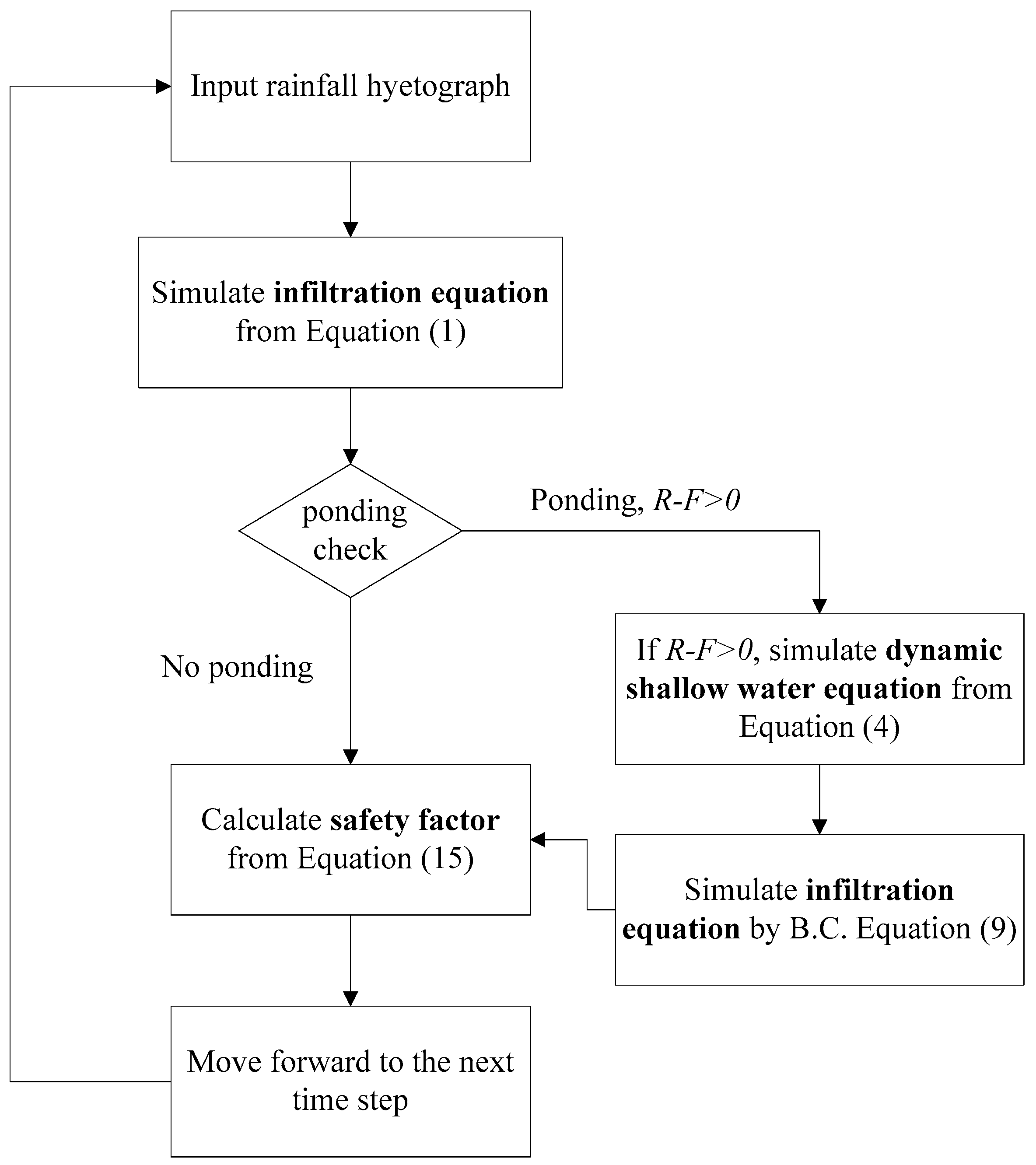
The details of the algorithm of the 2D-SWE module can be found in [23], and details of the soil failure module can be found in [11] or [7]. An iterative procedure (Figure 1) is adopted to solve Equations (1) to (12). The iterative approach alternates the solutions of the infiltration and shallow water equations at each time step until convergence is reached. Firstly, the groundwater pressure head of a hillslope is obtained by assuming that the infiltration rate equals the rainfall intensity, as presented in Equation (8). If the pressure head on the slope surface is less than or equal to zero, then ponding does not occur, such that the calculating procedure moves forward to the next time-step. However, if the calculated pressure head on the slope surface is larger than zero, that is, R – F > 0, then the 2D-SWE given by Equations (4) to (6) needs to be solved. Thus, the water depth will become a boundary condition of infiltration for recalculation within the same time step. Finally, the calculated pore water pressures in the slopes are substituted into Equation (15), and then FS is obtained.

3. Numerical Model Verification

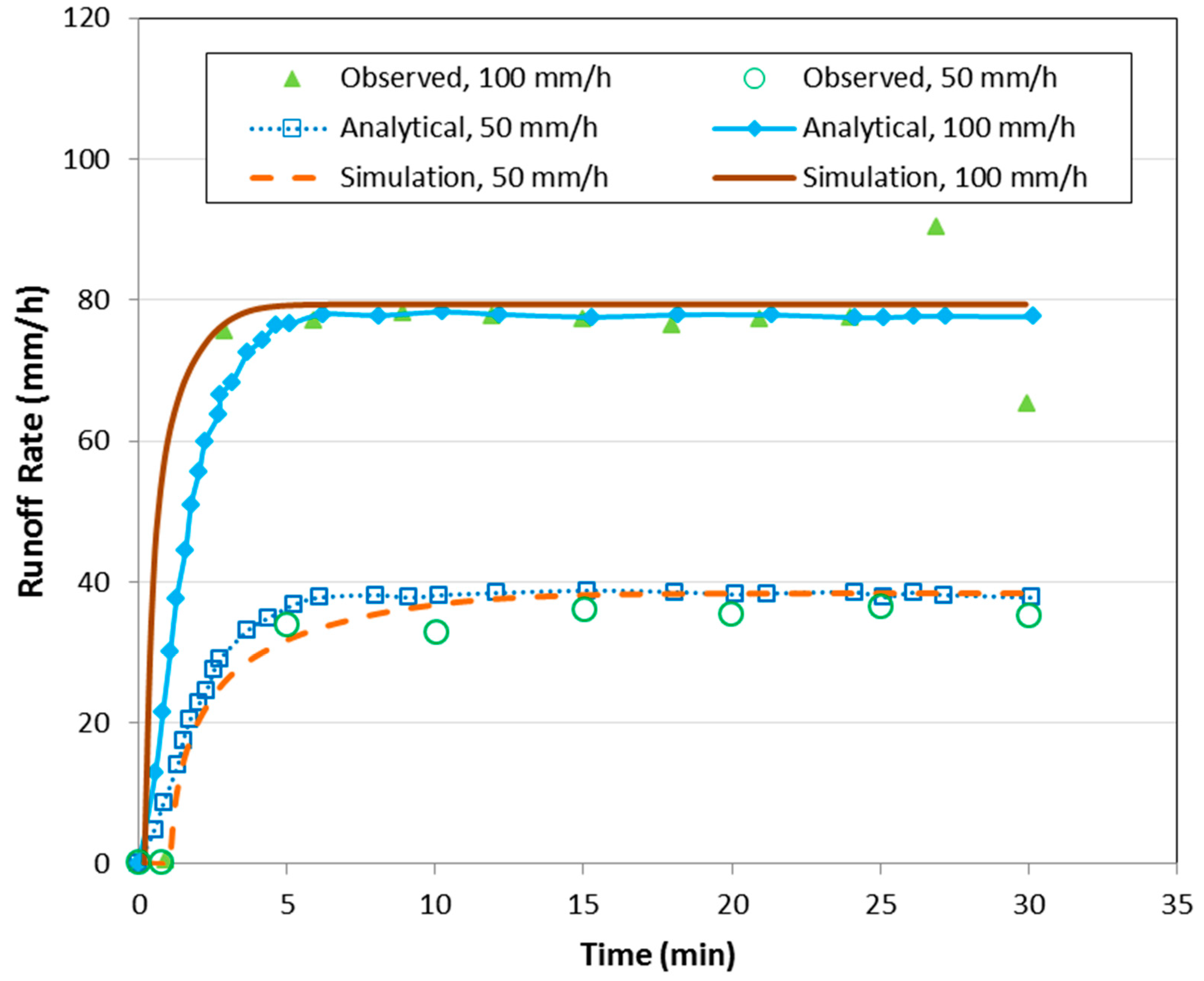
To verify the rainfall–runoff–infiltration module, the performance of the model has been compared with the experimental results of Singer and Walker [24], while the analytical solution of Govindaraju and Kavvas [25] is used to verify the model as well.

The test setup consisted of a rectangular laboratory soil flume (3.0 m × 0.55 m) with a 9% slope and a rainfall simulator. In the flume, 200 kg of moist fresh soil (bulk density of 1200 kg/m³) was packed with an 80 mm thickness for each rainfall event. The median diameter of the soil was 2.0 × 10⁻⁵ m.

To compare the performance of the model, uniform cells of 0.05 m × 0.05 m were used. The duration of each run was 30.0 min for two different cases of rainfall intensity: 50 mm/h and 100 mm/h. The Manning roughness coefficient was assumed to be constant at 0.02 over the entire rainfall event. To calculate the infiltration, certain parameters are required to be set: the wetting front capillary pressure head is 0.006 m, the soil water content deficit is 0.2, and the saturated hydraulic conductivity for the 50 mm/h and 100 mm/h rainfall intensity cases is 3.25 × 10⁻⁶ m/s and 5.0 × 10⁻⁶ m/s, respectively, following the results of Nord and Esteves [26].

Figure 2 shows a comparison of the model simulation with the observed discharge hydrographs and analytical results. Good agreement between the calculated results and the reference values can be seen.

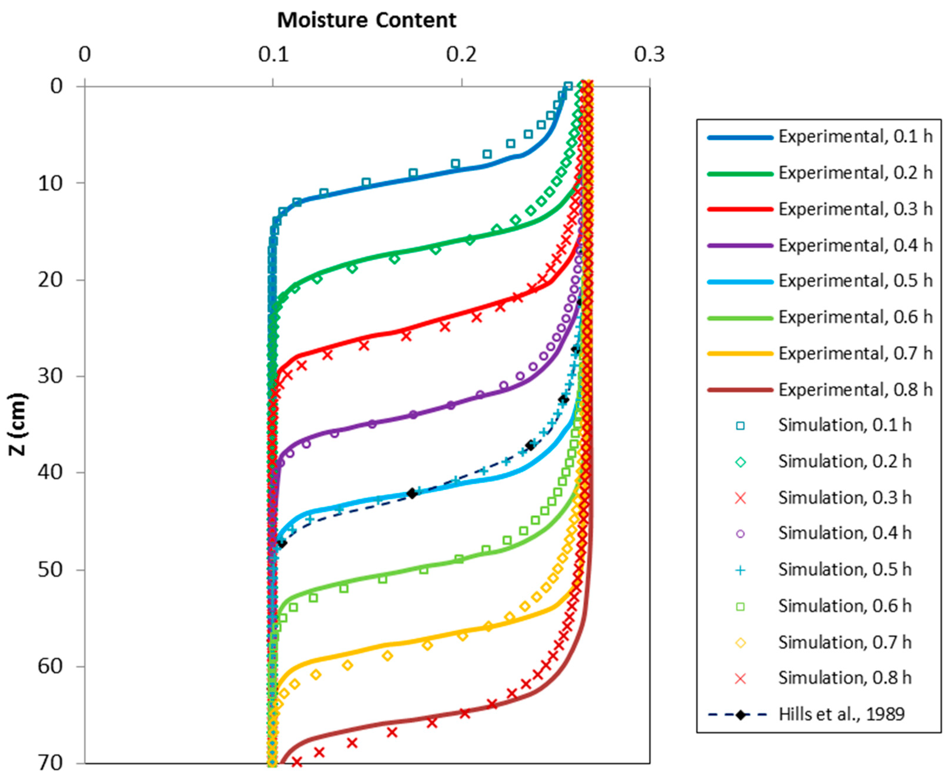
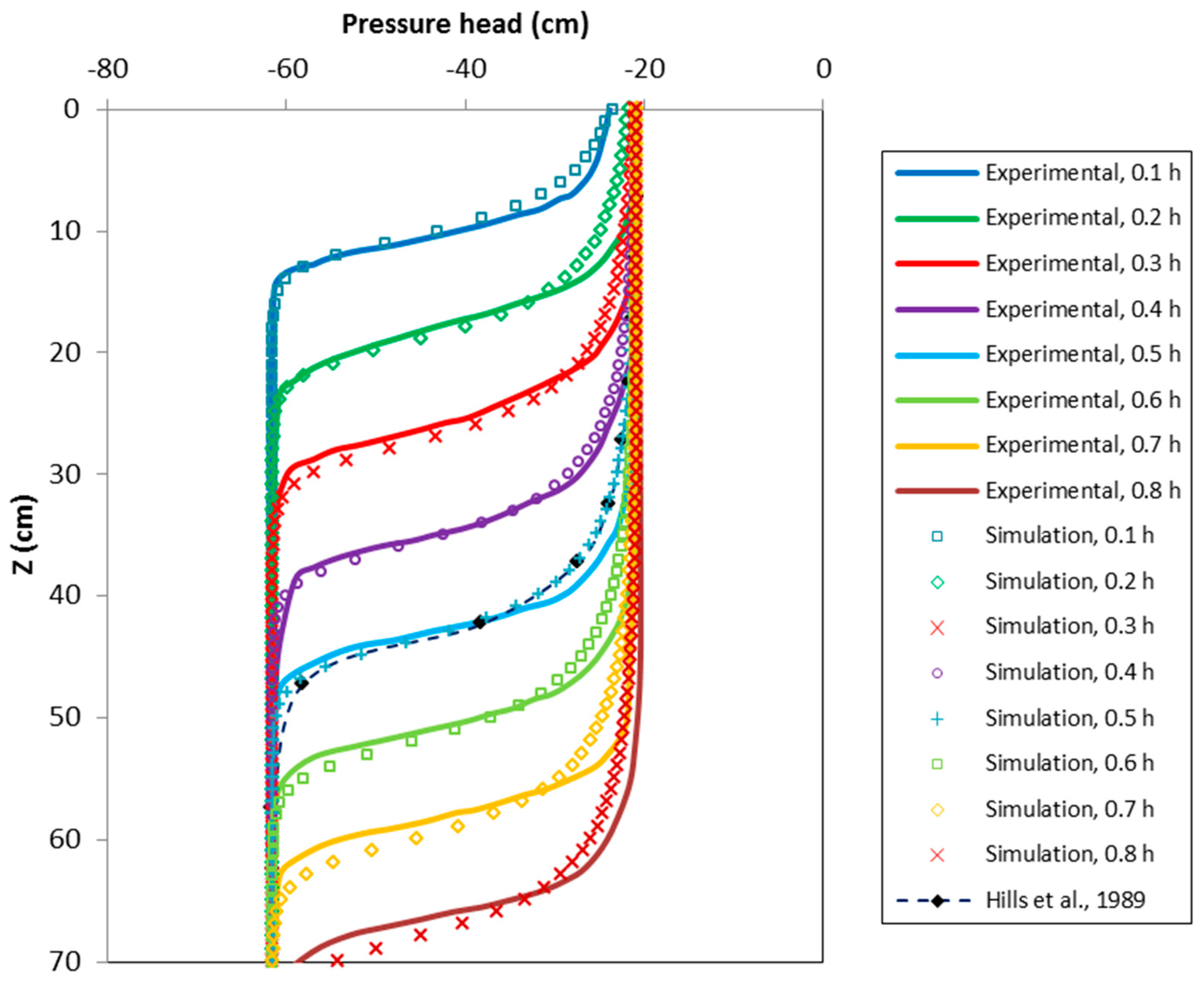
Another laboratory infiltration experiment we adopt to verify the calculation of water content and water pressure was originally designed by Haverkamp et al. [27]. The test comprised a uniform laboratory scale soil column (bulk density of 1.66 g/cm³) with a constant water flux (q_z = 13.69 cm/h) at the soil surface and a constant water pressure at the end of the soil column. The changes of water content at different depths were obtained. This verification has also been made by other numerical models, for example, Hills et al. [28]. The experimental water content profiles and the simulation results are presented in Figure 3 and the pressure head profiles in Figure 4. The comparisons show good agreement, and no significant difference from the measured water contents is found.

4. Description of Case Study

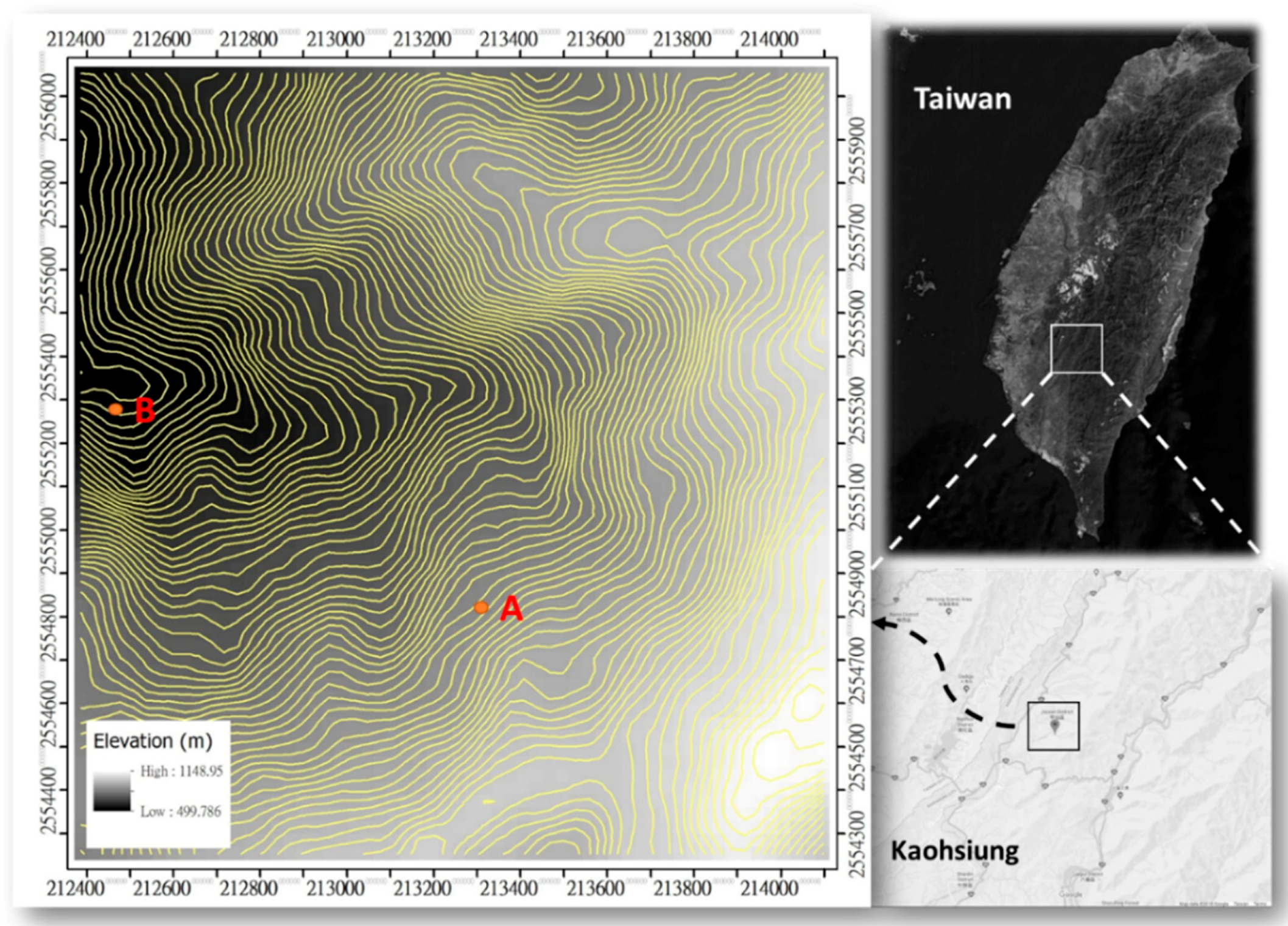
To observe the effects of rainfall runoff in a regional simulation, a real-world small catchment topography (approximately 3 km²) and a real storm hyetograph were applied. Figure 5 shows the topography of Beng-Ping-Keng (Kaohsiung), a mountainous area in southern Taiwan that is hit by, on average, 3–4 typhoons per year.

There are a total of 61 × 58 uniform cells with a resolution of 30 m in the modeling area (the resolution of the digital elevation model (DEM) is 30 m as well). The maximum and minimum elevations of the catchment are 1149.0 m and 499.8 m, respectively. The soil is classified as sandy loam. The depth of the pervious layer is assumed to be 1.3 m at every slope, and the initial groundwater table is 2.0 m below the ground surface of the hillslope. The soil parameters we use in the case study are listed as follows: $K_s=2.84\times {10}^{-6}m/s$; ${\theta }_s$ = 0.5; ${\theta }_r$ = 0.24; N = 1.8; M = 0.556; $\xi$ = 0.008; c’ = 4 kpa; $\varphi \prime$ = 26°; and $G_s$ = 2.65.

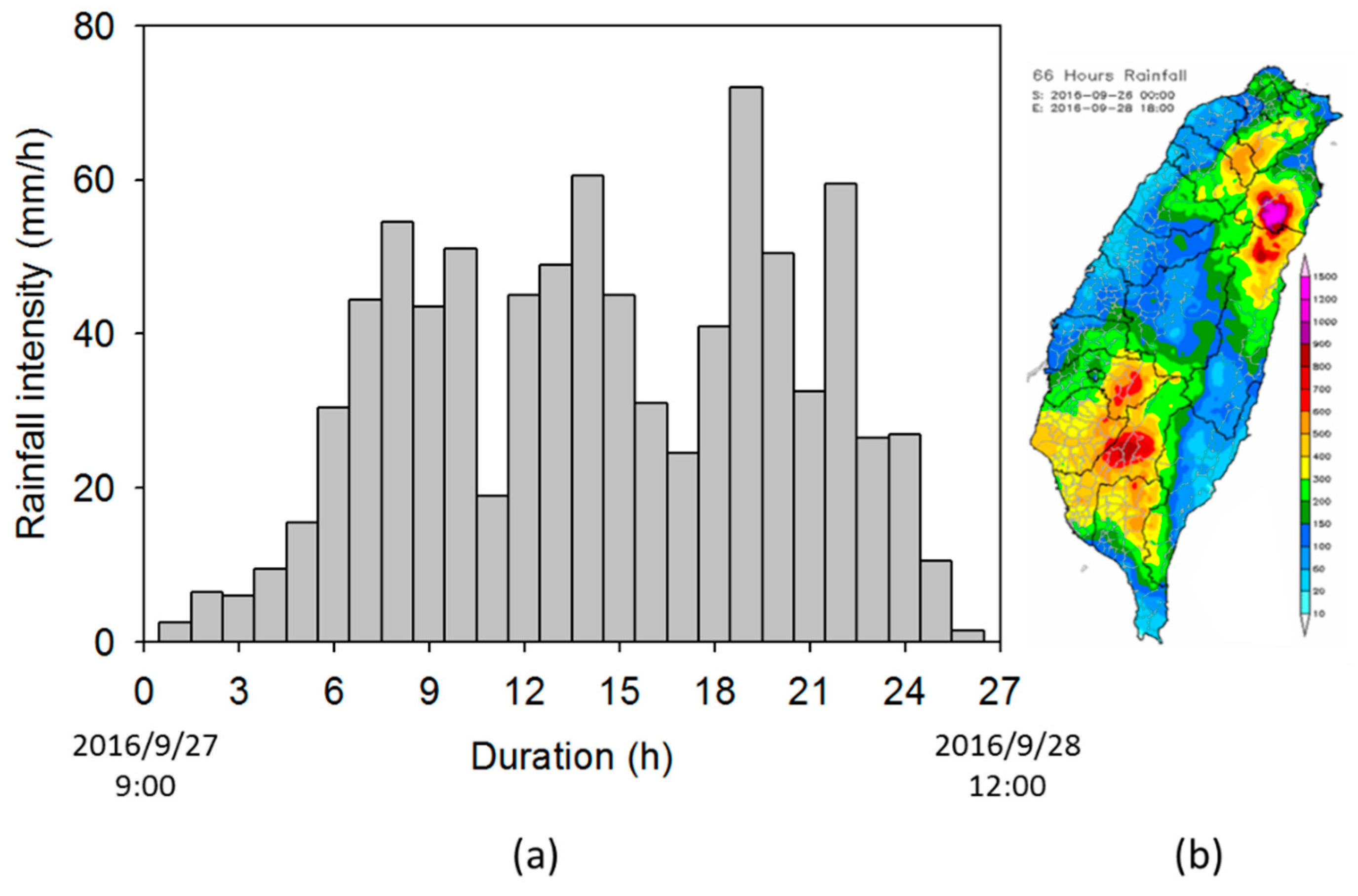
A storm that hit on 27 September 2016 is chosen as the simulation scenario. The storm, Typhoon Meigi, caused several flooding and landslide disasters in southern Taiwan, which resulted in significant economic losses and road closures. According to the meteorological data, the accumulated precipitation in the study area was higher than 900 mm during the storm, which had a duration of approximately 27 h. The recorded hyetograph for the catchment is presented in Figure 6. This storm event can be divided into three parts: The first event lasted 11 h from the onset of the storm (09:00 to 20:00 on 27 September), and the second and third events lasted 6 h (from 20:00 on 27 September to 02:00 on 28 September) and 10 h (from 02:00 to 12:00 on 28 September), respectively. The peak of each part of the rainfall event occurs at the eighth hour (54.5 mm/h), the fourteenth hour (60.5 mm/h), and the nineteenth hour (72.0 mm/h).

5. Results

5.1. Water Depth

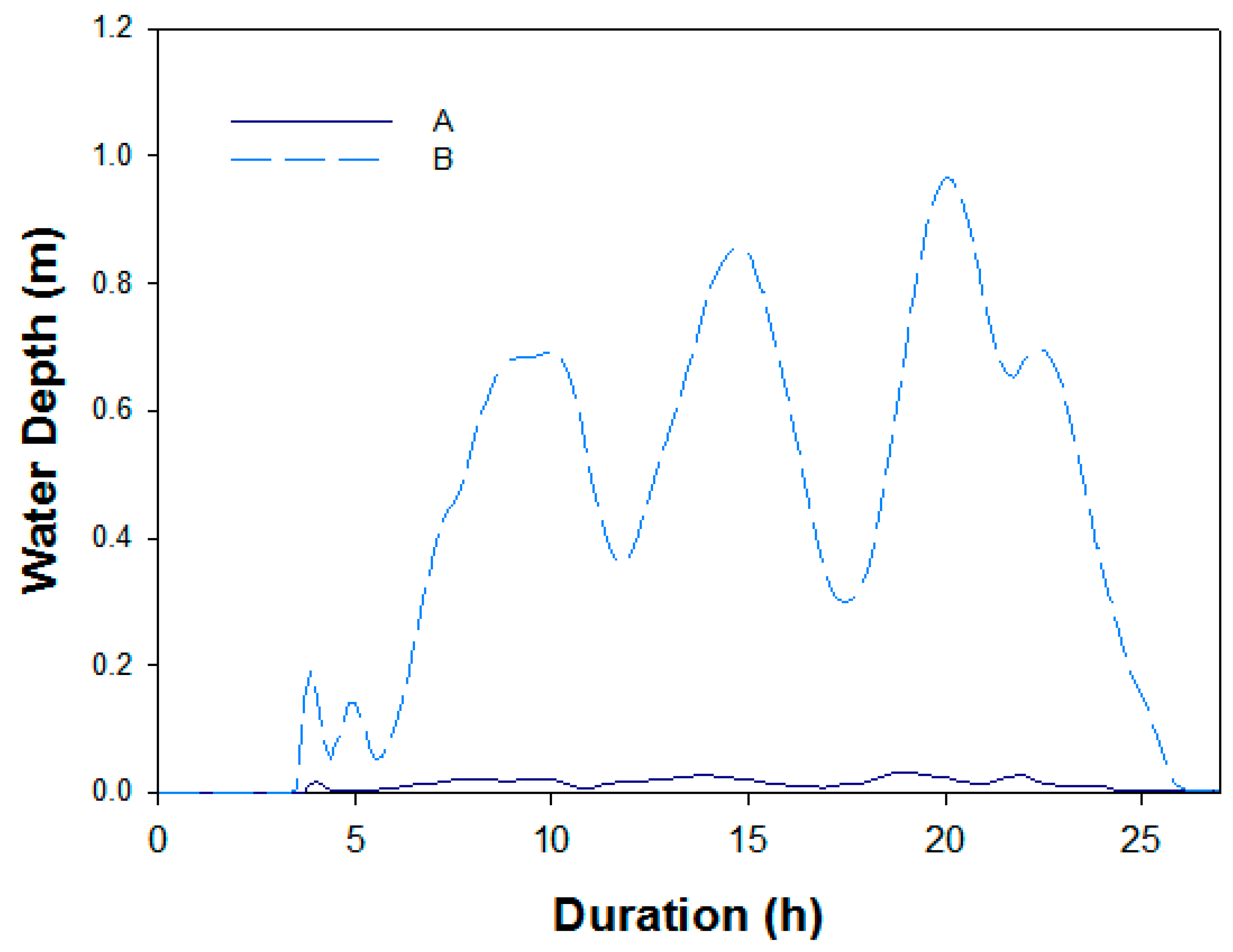
The simulated water depth hydrographs extracted from two different locations in the study area (see Figure 5, Locations A and B) are illustrated in Figure 7. The water depth at location A during the entire event is very shallow compared to the water depth at location B, which is at the toe of a hillslope and is a short distance to the outlet of the whole catchment. From the hydrograph of location B, three peaks can be clearly recognized. Figure 6 and Figure 7 show a lag of approximately an hour between the peak of the rainfall event and the maximum discharge.

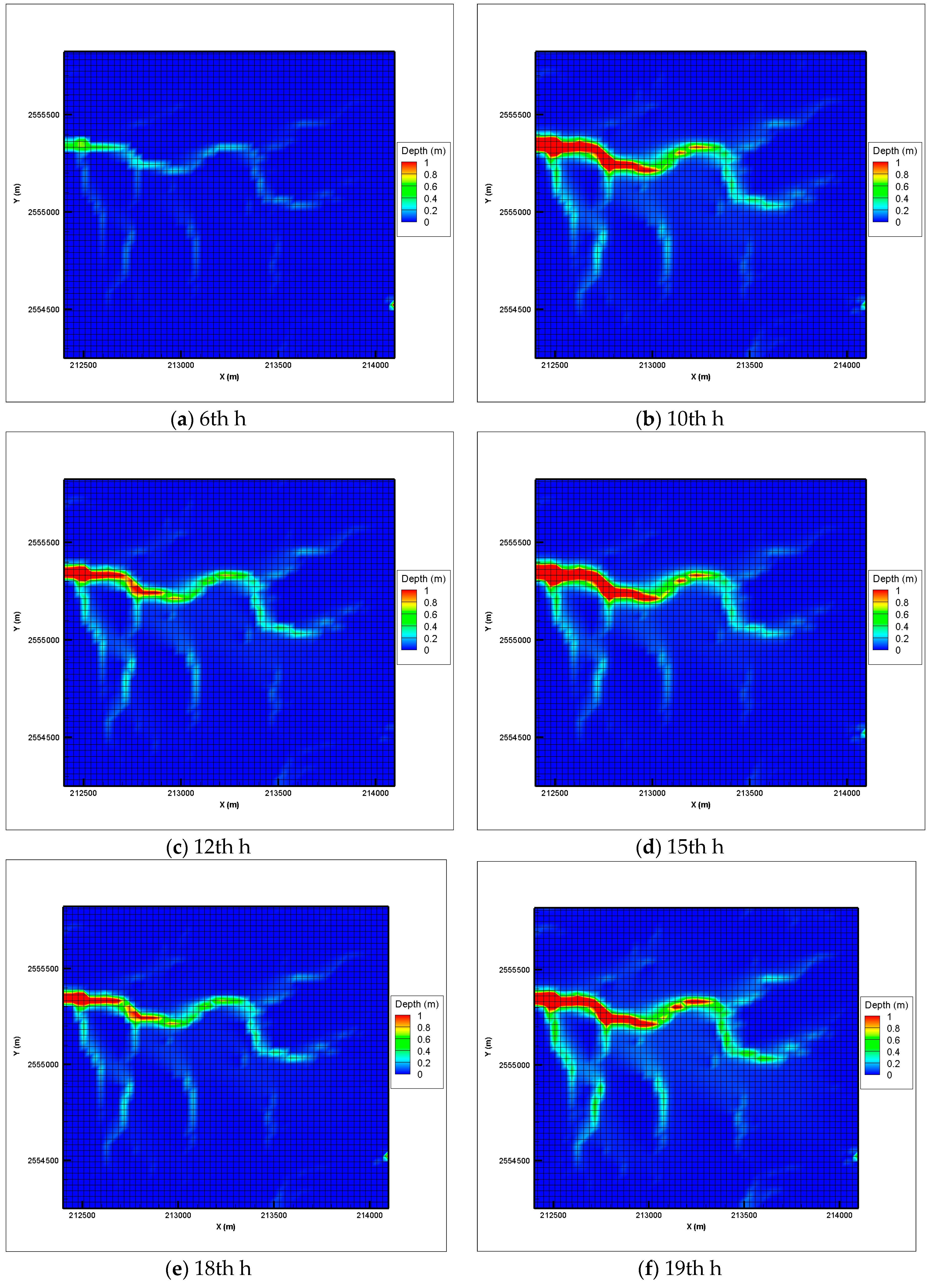
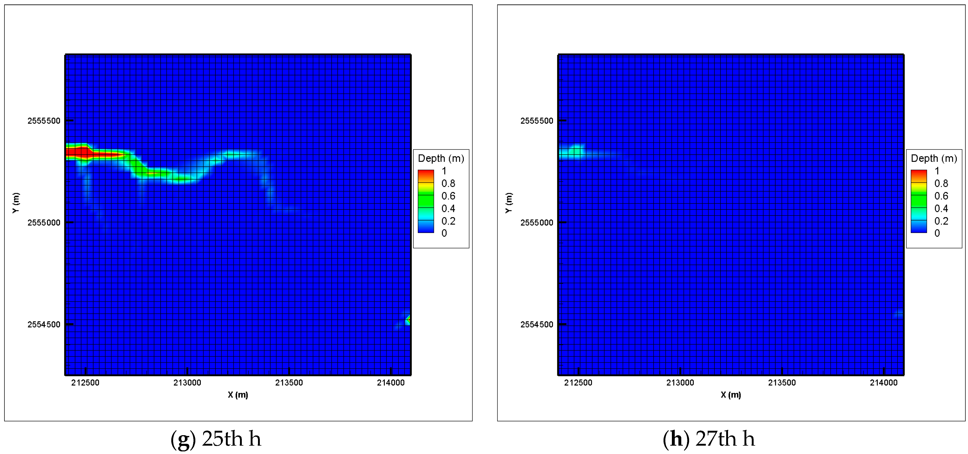
Figure 8 shows the simulation results of the water depth distribution in the catchment. After the surface soils are saturated, the flow converges in the rills of the catchment, and a water path can clearly be observed. For the case of typhoon Meigi, the highest water depth downstream is over 1 m, while the water depth on the slopes of the catchment is largely still at minimal values.

5.2. Factor of Safety

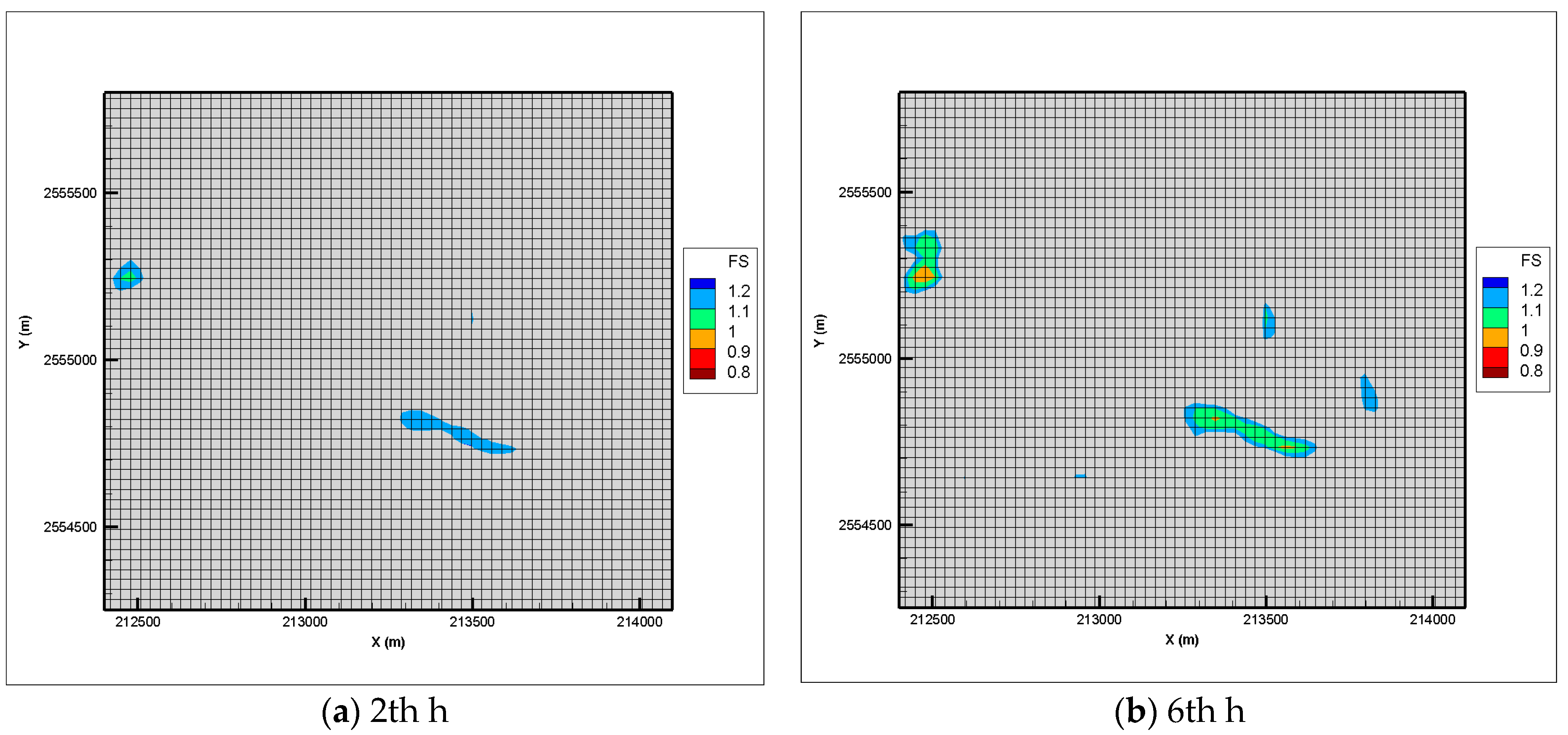
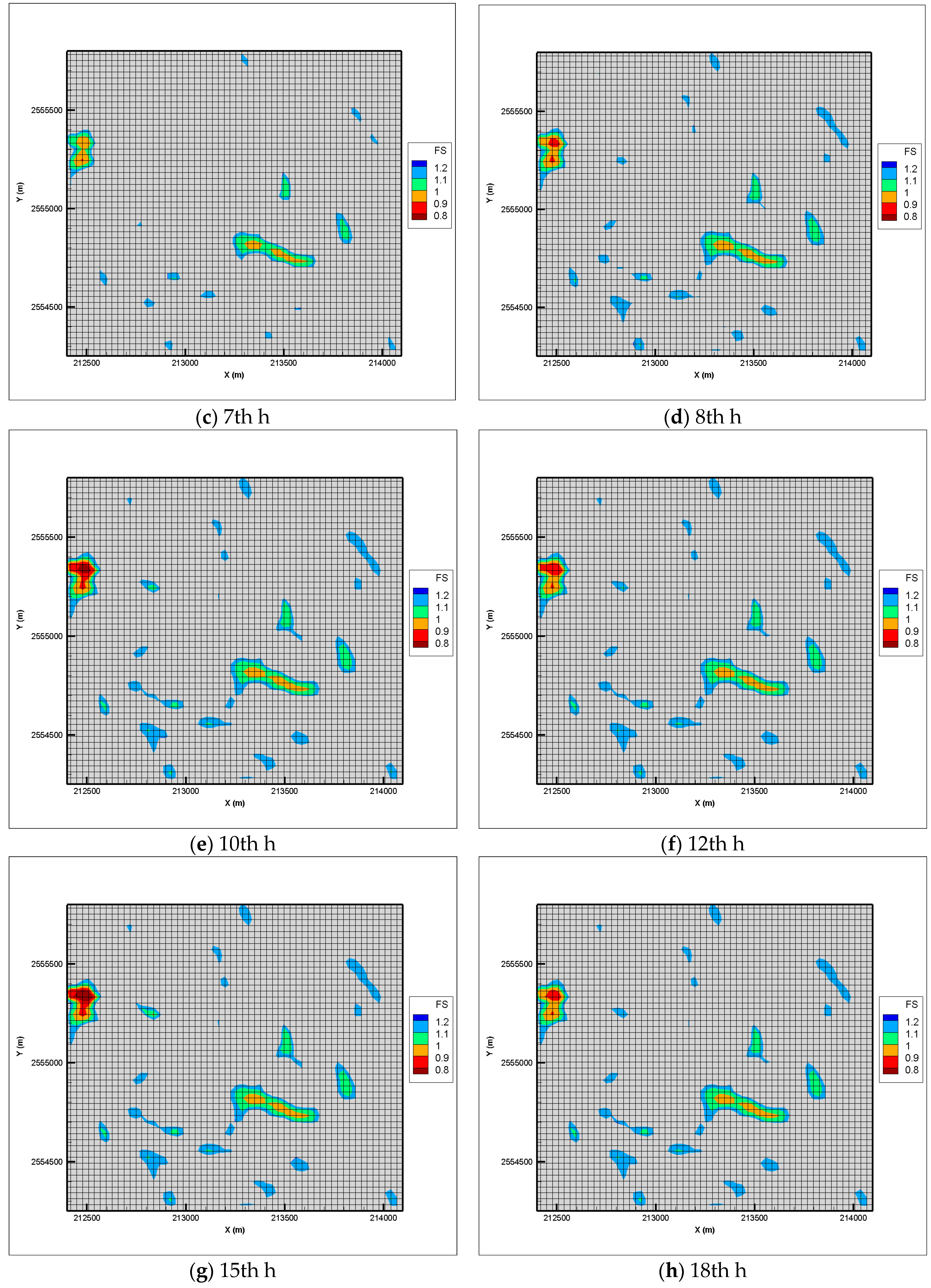
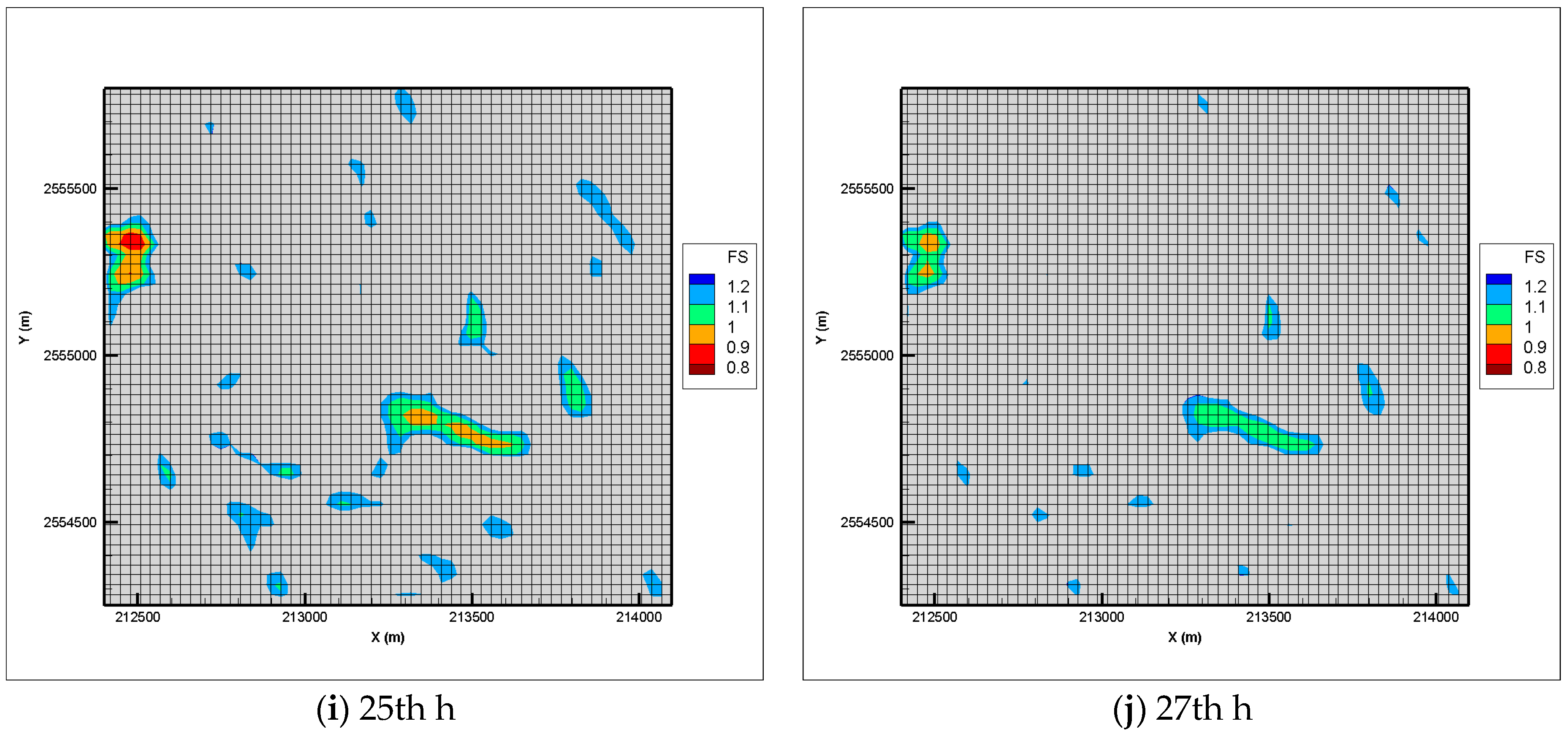
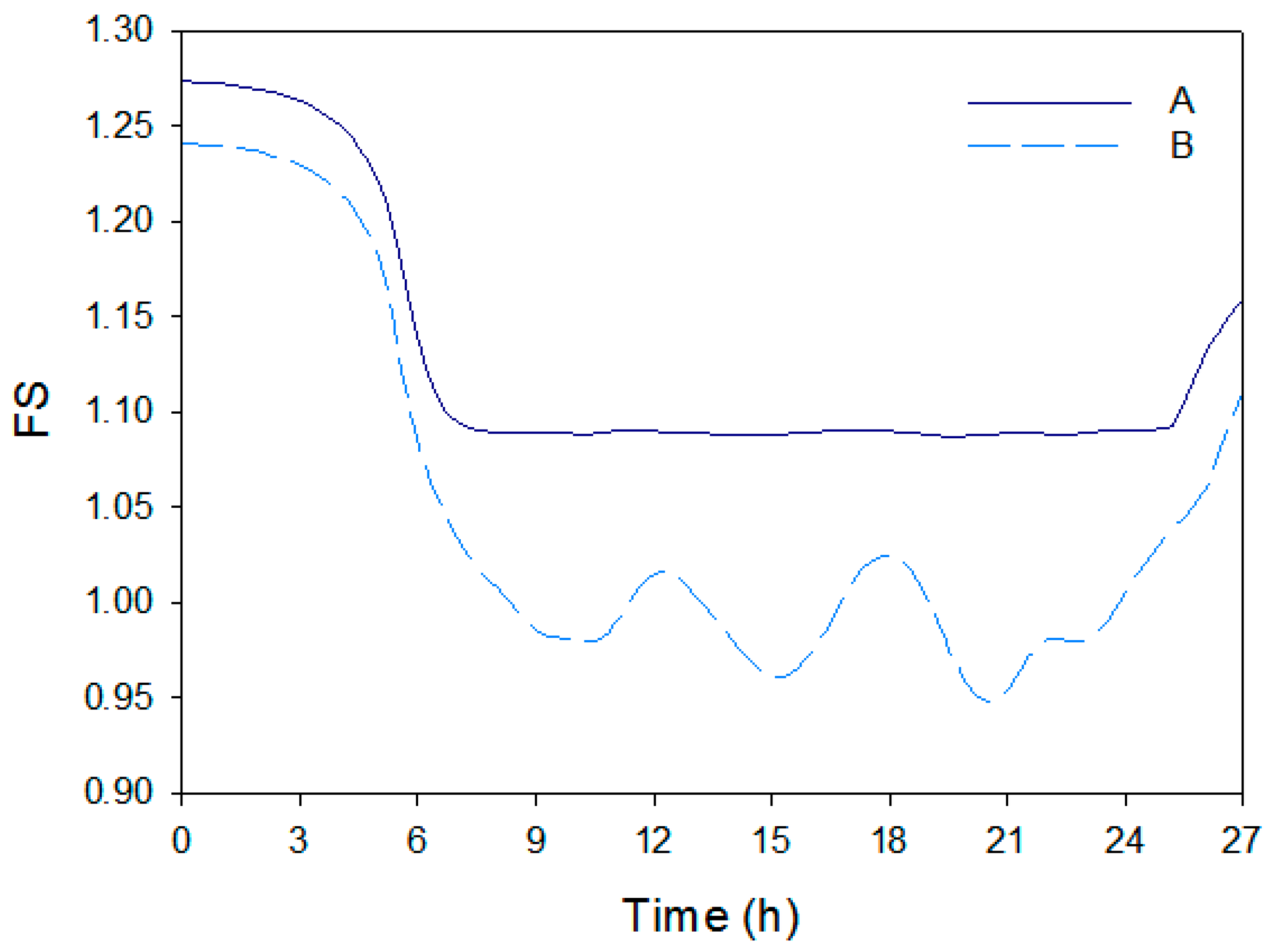
The calculated FS of every cell is shown in Figure 9. The gray color indicates FS > 1.2. During the initial hours, the areas where FS < 1.2 expand gradually with time (Figure 9a–d), and in the left (downslope) and the middle regions of the simulated domain, some cells start becoming unstable (FS < 1) from the 6th hour (Figure 9b). At the beginning of the storm, the FS is mainly affected by infiltration. Between the 8th and 25th hours, the FS of these cells continues to fluctuate over time, while the rest exhibits no significant change. For example, the FS of the area on the downslope increased from the 8th hour to the 10th hour (Figure 9d–e) and from the 12th hour to the 15th hour (Figure 9f–g), and decreased from the 10th hour to the 12th hour (Figure 9e–f) and from the 15th hour to the 18th hour (Figure 9g–h). Finally, when the rain stops, most cells return to a stable form, except for some in the outlet of the catchment (Figure 9j).

From the results above, we can see that with the same hyetograph and the same soil properties, the FS of some cells changes continuously, while that of some remains constant. To further observe and analyze this phenomenon, Locations A and B are selected as reference points. The FS of Locations A and B during Typhoon Meigi 1 m below the ground is shown in Figure 10. The FS of both spots decreases dramatically in the first six hours, which is consistent with Figure 9. In contrast with Location A, it is clear that the FS at Location B fluctuates between 0.95 and 1.05 over time and reaches the lowest values at the 10th, 15th, and 20th hours, consistent with the water depth variation in Figure 7. The reason for these different trends is discussed in the next section.

6. Discussion

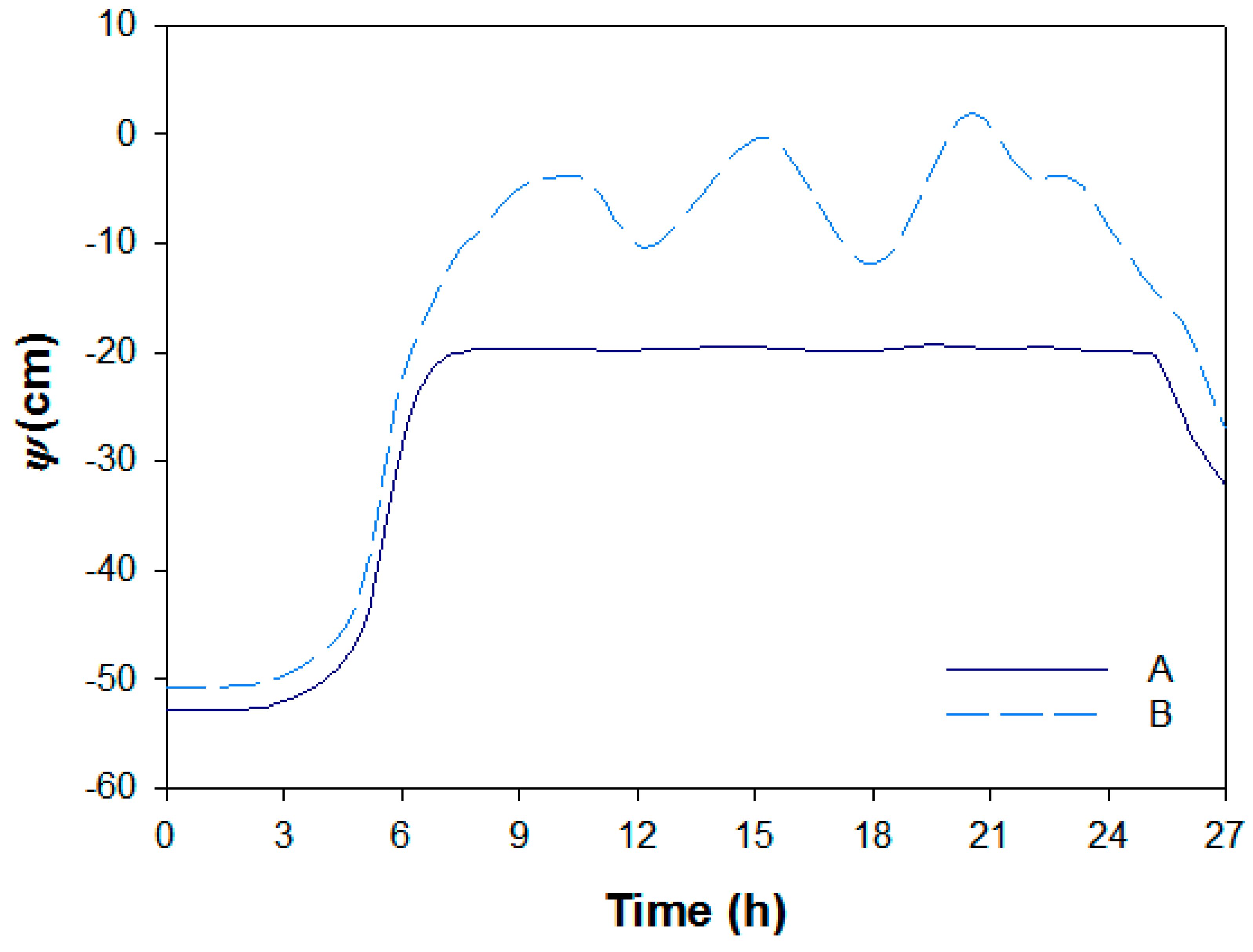
Equation (15) shows that the FS(Z) is defined by the following variables: $\alpha$, $\varphi \prime$, $c\prime$, $\chi$, $\overline{\gamma }$, ${\psi }_c$, and ${\psi }_P$. Among these variables, $\alpha$, $\varphi \prime$, and $c\prime$, are dependent on geographical or soil properties, and the $\chi$ and $\overline{\gamma }$ are approximately constant when the soil is nearly saturated; hence, the FS is mainly affected by the pressure head variables, ${\psi }_c$ and ${\psi }_P$. Moreover, after the ground soil is saturated, these variables vary with the depth of surface water. The inference can be verified by the pressure head calculations of Locations A and B.

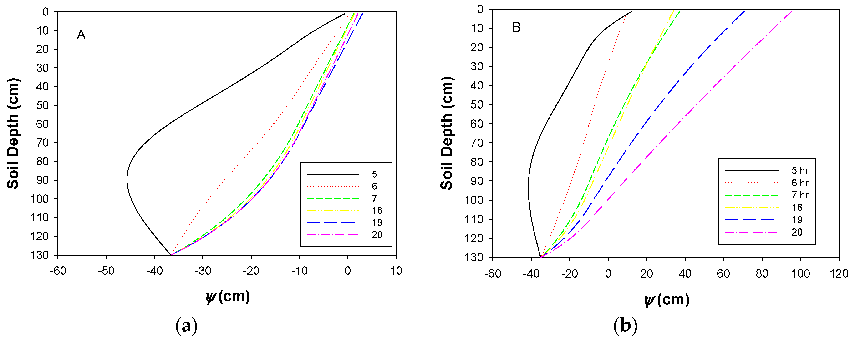
The pressure head of Locations A and B 1 m below the ground is presented in Figure 11. Obviously, the trends of the pressure head are highly similar to the trend of FS. During the first 7 h of the storm event, the pressure head increased gradually. Then, similar to the trends of the FS, the pressure head of Location A stays constant, while that of Location B varies with time. The simulation results of the pressure head versus depth distributions are illustrated in Figure 12. Because the pervious base is located at a depth of 1.3 m, the location of both heads is constant at a depth of 1.3 m. The head distributions at the fifth hour of both spots are similar because the ground soil is very close to saturation (i.e., the pressure head is larger than zero).

Furthermore, at Location A, the pressure head distribution has no noticeable change after the seventh hour. This is because there is only a small variation in the surface water depth (see Figure 7). However, in both Figure 11 and Figure 12, the pressure head at Location B increases continuously, owing to the variation of the depth of water that is collected from the upper slopes. The difference between Locations A and B in Figure 11 and Figure 12 demonstrates the effect of surface water depth. In summary, from the simulation results, it is clear that the surface water depth causes the increases of the water pressure head, and further affects the FS of the slope.

7. Conclusions

The present study focuses on the influence of runoff on slope stability because infiltration has been widely considered as the main factor causing shallow landslides, whereas the effect of runoff is not extensively discussed. Therefore, a physical-process-based numerical model that can properly demonstrate the process of the infiltration, runoff, and slope stability is necessary. To illustrate the influence of rainfall–runoff, a small catchment in Kaohsiung, Taiwan, is chosen as an example. The simulation shows the variations of water depth and FS during a 27-hour storm event, Typhoon Meigi.

From the plane distributions of the simulated water depth and FS, we see that the surface soil remains saturated, but the FS of some cells varies constantly, and it is most likely to appear in the downstream area where the runoff converges. By analyzing variables in the FS equation, we summarize that the decreasing FS downstream is due to the increasing pressure head at that position; and the increment is caused by the accumulated depth of the surface runoff. The variations over time of FS and the pressure head at two selected locations show similar changing trends, thus verifying the conclusion. Therefore, when analyzing the regional slope stability, it is suggested to take the influence of runoff into account. That aside, using hydrodynamic shallow water equations may have the advantage of calculating water depth accurately and provide a good foundation to evaluate the influence of runoff on shallow landslides.

References

- Rahardjo, H.; Lim, T.; Chang, M.; Fredlund, D. Shear-strength characteristics of a residual soil. Can. Geotech. J. 1995, 32, 60–77. [Google Scholar] [CrossRef]
- Iverson, R.M. Landslide triggering by rain infiltration. Water Resour. Res. 2000, 36, 1897–1910. [Google Scholar] [CrossRef] [Green Version]
- Baum, R.L.; Savage, W.Z.; Godt, J.W. TRIGRS–A Fortran Program for Transient Rainfall Infiltration and Grid-Based Regional Slope-Stability Analysis, Version 2.0; US Geological Survey: Reston, VA, USA, 2008.
- Tsai, T.-L.; Yang, J.-C. Modeling of rainfall-triggered shallow landslide. Environ. Geol. 2006, 50, 525–534. [Google Scholar] [CrossRef]
- Tarantino, A.; Bosco, G. Role of soil suction in understanding the triggering mechanisms of flow slides associated with rainfall. In Debris-Flow Hazards Mitigation: Mechanics, Prediction, and Assessment, Proceedings of the Second International Conference on Debris-Flow Hazards Mitigation, Taipei, Taiwan, 16–18 August 2000; A.A. Balkema: Rotterdam, The Netherlands, 2000; pp. 81–88. [Google Scholar]
- Collins, B.D.; Znidarcic, D. Stability Analyses of Rainfall Induced Landslides. J. Geotech. Geoenviron. Eng. 2004, 130, 362–372. [Google Scholar] [CrossRef]
- Tsai, T.-L.; Chen, H.-E.; Yang, J.-C. Numerical modeling of rainstorm-induced shallow landslides in saturated and unsaturated soils. Environ. Geol. 2008, 55, 1269–1277. [Google Scholar] [CrossRef]
- Fredlund, D.; Morgenstern, N.R.; Widger, R. The shear strength of unsaturated soils. Can. Geotech. J. 1978, 15, 313–321. [Google Scholar] [CrossRef]
- Tsai, T.-L. The influence of rainstorm pattern on shallow landslide. Environ. Geol. 2008, 53, 1563–1569. [Google Scholar] [CrossRef]
- Tsai, T.-L.; Wang, J.-K. Examination of influences of rainfall patterns on shallow landslides due to dissipation of matric suction. Environ. Earth Sci. 2011, 63, 65–75. [Google Scholar] [CrossRef]
- Chen, H.-E.; Tsai, T.-L.; Yang, J.-C. Threshold of slope instability induced by rainfall and lateral flow. Water 2017, 9, 722. [Google Scholar] [CrossRef]
- Chan, H.-C.; Chen, P.-A.; Lee, J.-T. Rainfall-induced landslide susceptibility using a rainfall–runoff model and logistic regression. Water 2018, 10, 1354. [Google Scholar] [CrossRef]
- Muntohar, A.S.; Liao, H.-J. Rainfall infiltration: Infinite slope model for landslides triggering by rainstorm. Nat. Hazards 2010, 54, 967–984. [Google Scholar] [CrossRef]
- Gavin, K.; Xue, J. A simple method to analyze infiltration into unsaturated soil slopes. Comput. Geotech. 2008, 35, 223–230. [Google Scholar] [CrossRef]
- Tian, D.; Liu, D. A new integrated surface and subsurface flows model and its verification. Appl. Math. Model. 2011, 35, 3574–3586. [Google Scholar] [CrossRef]
- Tong, F.-G.; Tian, B.; Liu, D.-F. A coupling analysis of slope runoff and infiltration under rainfall. Rock Soil Mech. 2008, 29, 1035. [Google Scholar]
- Querner, E. Description and application of the combined surface and groundwater flow model MOGROW. J. Hydrol. 1997, 192, 158–188. [Google Scholar] [CrossRef]
- Van Genuchten, M.T. A closed-form equation for predicting the hydraulic conductivity of unsaturated soils. Soil Sci. Soc. Am. J. 1980, 44, 892–898. [Google Scholar] [CrossRef]
- Zhang, W.; Cundy, T.W. Modeling of two-dimensional overland flow. Water Resour. Res. 1989, 25, 2019–2035. [Google Scholar] [CrossRef]
- Vreugdenhil, C.B. Numerical Methods for Shallow-Water Flow; Springer Science & Business Media: Berlin, Germany, 2013; Volume 13. [Google Scholar]
- Vanapalli, S.; Fredlund, D. Empirical procedures to predict the shear strength of unsaturated soils. In Proceedings of the Eleventh Asian Regional Conference on Soil Mechanics and Geotechnical Engineering, Seoul, Korea, 16–20 August 1999; pp. 93–96. [Google Scholar]
- Celia, M.A.; Bouloutas, E.T.; Zarba, R.L. A general mass conservative numerical solution for unsaturated flow equation. Water Resour. Res. 1990, 26, 14. [Google Scholar] [CrossRef]
- Tsakiris, G.; Bellos, V. A numerical model for two-dimensional flood routing in complex terrains. Water Resour. Manag. 2014, 28, 1277–1291. [Google Scholar] [CrossRef]
- Singer, M.J.; Walker, P.H. Rainfall runoff in soil erosion with simulated rainfall, overland flow and cover. Soil Res. 1983, 21, 109–122. [Google Scholar] [CrossRef]
- Govindaraju, R.S.; Kavvas, M.L. Modeling the erosion process over steep slopes: Approximate analytical solutions. J. Hydrol. 1991, 127, 279–305. [Google Scholar] [CrossRef]
- Nord, G.; Esteves, M. PSEM_2D: A physically based model of erosion processes at the plot scale. Water Resour. Res. 2005, 41, W08407. [Google Scholar] [CrossRef]
- Haverkamp, R.; Vauclin, M.; Touma, J.; Wierenga, P.; Vachaud, G. A comparison of numerical simulation models for one-dimensional infiltration 1. Soil Sci. Soc. Am. J. 1977, 41, 285–294. [Google Scholar] [CrossRef]
- Hills, R.; Porro, I.; Hudson, D.; Wierenga, P. Modeling one-dimensional infiltration into very dry soils: 1. Model development and evaluation. Water Resour. Res. 1989, 25, 1259–1269. [Google Scholar] [CrossRef]
Figure 1.
Flow chart of the model developed in this study.
Figure 2.
Model results: Calculated runoff rate and reference data (the analytical solutions were obtained from Govindaraju and Kavvas [25], while the observed experimental results were from Singer and Walker [24]).
Figure 3.
Comparison of model results: The water content profiles (Haverkamp et al. [27] and Hills et al. [28]).
Figure 4.
Comparison of model results: The pressure head profiles (Haverkamp et al. [27] & Hills et al. [28]).
Figure 5.
Catchment topography of the numerical experiment.
Figure 6.
Meteorological data of Typhoon Meigi: (a) Hyetograph in the study area; (b) spatial distribution of accumulated rainfall amount (Source: National Science and Technology Center for Disaster Reduction, Taiwan).
Figure 7.
Simulation results of water depth on slope surface at Locations A and B during Typhoon Meigi.
Figure 8.
Simulation results of water depth with time during Typhoon Meigi.
Figure 9.
Simulated results of the factor of safety (FS) varying with time during the Typhoon Meigi (gray color represents FS > 1.2).
Figure 10.
Simulated results of FS at Locations A and B during Typhoon Meigi (1 m below ground).
Figure 11.
Simulated results of groundwater (pressure head varied with time, 1 m below ground at Locations A and B during Typhoon Meigi).
Figure 12.
Simulated results of groundwater pressure heads at (a) Location A and (b) Location B.
© 2019 by the authors. Licensee MDPI, Basel, Switzerland. This article is an open access article distributed under the terms and conditions of the Creative Commons Attribution (CC BY) license (http://creativecommons.org/licenses/by/4.0/).
Share and Cite
MDPI and ACS Style
Chiu, Y.-Y.; Chen, H.-E.; Yeh, K.-C. Investigation of the Influence of Rainfall Runoff on Shallow Landslides in Unsaturated Soil Using a Mathematical Model. Water 2019, 11, 1178. https://doi.org/10.3390/w11061178
AMA Style
Chiu Y-Y, Chen H-E, Yeh K-C. Investigation of the Influence of Rainfall Runoff on Shallow Landslides in Unsaturated Soil Using a Mathematical Model. Water. 2019; 11(6):1178. https://doi.org/10.3390/w11061178
Chicago/Turabian StyleChiu, Yen-Yu, Hung-En Chen, and Keh-Chia Yeh. 2019. "Investigation of the Influence of Rainfall Runoff on Shallow Landslides in Unsaturated Soil Using a Mathematical Model" Water 11, no. 6: 1178. https://doi.org/10.3390/w11061178
Note that from the first issue of 2016, this journal uses article numbers instead of page numbers. See further details here.