Experimental Analysis of the Influence of Aeration in the Energy Dissipation of Supercritical Channel Flows
by
 , , ,
, , ,
Juan José Rebollo
1,2,* ,
,
David López
1,
Luis Garrote
2,
Tamara Ramos
1,
Rubén Díaz
3 and
Ricardo Herrero
1 1
Hydraulic Laboratory of the Hydrographical Study Center, CEDEX, Ministry of Public Works and Transport, 28005 Madrid, Spain
2
Department of Civil Engineering: Hydraulics, Energy and Environment, Universidad Politécnica de Madrid, 28040 Madrid, Spain
3
Department of Infrastructures Planning, Ministry of Public Works and Transport, 28071 Madrid, Spain
*
Author to whom correspondence should be addressed.
Water 2019, 11(3), 576; https://doi.org/10.3390/w11030576
Submission received: 8 February 2019
/
Revised: 13 March 2019
/
Accepted: 15 March 2019
/
Published: 20 March 2019
(This article belongs to the Special Issue Hydrological and Hydro-Meteorological Extremes and Related Risk and Uncertainty)
Abstract
:Energy dissipation structures play an important role in flood risk management. Many variables need to be considered for the design of these structures. Aeration has been one of the more studied phenomena over the last years, due to its influence in the performance of hydraulic structures. The purpose of the work presented in this article is to experimentally characterize the effects of aeration on boundary friction in supercritical and fully turbulent flows. The physical model used to analyze the aeration effects consists of a spillway chute 6.5 m high and a stilling basin of 10 m length and 2 m high. A pump and compressor supply the water-air mixture and are controlled at the entrance by valves and flowmeters. The ensuing channel is monitored to determine the velocity profile and air concentration of the flow into the stilling basin. The average values of both variables and Manning’s coefficient along the channel are used to determine the relation between air concentration and energy dissipation by friction. A velocity increase with greater air entrainment has been found in all scenarios since friction is the main energy dissipation mechanism in open channels flow. Finally, an equation is proposed to characterize this evolution based on the results obtained.
1. Introduction
Climate change impacts may compromise the security of hydraulic structures by exacerbated extreme hydrological regimes and higher flood flows. Moreover, current society demands increasing safety standards in dam hydraulic outlets due to their effects on the social welfare and economic stability. As a consequence, it may be necessary to improve the hydraulic capacity of current dam outlets (including weirs, spillways and sluices). In this context, the Hydraulic Laboratory of CEDEX (Centre for Public Works Studies and Experimentation, Spain) is carrying out an experimental study on the influence of aeration over chutes and stilling basins in the framework of the EMULSIONA project, a research effort funded by the Spanish Ministry of Economy. The purpose of this study is to quantify the influence of aeration in the efficiency of energy dissipation structures [1,2,3]. Our analysis is based on a physical model test where flows with different air concentration may be produced. Considering the similarity criteria, these results are representative of those that would be obtained in a prototype hydraulic structure [4,5,6,7,8]. The first stage of the study is to characterize the hydraulic conditions of the intake flow in the stilling basin (depth, velocity and concentration). The analysis is focused on the effects of aeration on supercritical flows in the channel and on how the velocity field is modified according to different air concentration conditions. Results obtained during the experimental another coalysis of the spillway channel show a flow velocity increase with higher concentration. This phenomenon has been described before by Moñino [9] and Kramer [10]. Moreover, several studies have analyzed the effect of emulsionated flows in spillways with artificial aeration, as in Luna-Bahena [11] and Koen [12]. There are different proposals for energy dissipation mechanisms in open channel flows, depending on the regime analyzed. Turbulence and bubble effects play an important role in self-aerated open channels and stilling basins [13,14,15,16,17], but supercritical flows in spillways are highly influenced by roughness at the boundary [18]. The objective of the work presented in this article is to quantify the influence of aeration on the roughness boundary in high velocity and turbulent flows through friction mechanisms. Twelve flow scenarios were tested on the physical model with Froude numbers ranging between 5.5 and 6.5, representative values of flows in real spillways. In all tests, vertical velocity and air concentration profiles were measured at the channel axis. This information was used to determine the average Manning’s roughness coefficient in the channel and to establish a relationship between friction energy dissipation and air concentration.
2. Material and Methods
The experimental analysis was developed on a physical model built in the Hydraulic Laboratory of the Hydrographical Studies Centre (CEDEX, Spain). The following sections present the characteristics of the installation, the experimental design to reproduce the flow scenarios and the instrumentation used to take velocity and concentration measurements.
2.1. Physical Model and Supply Equipment
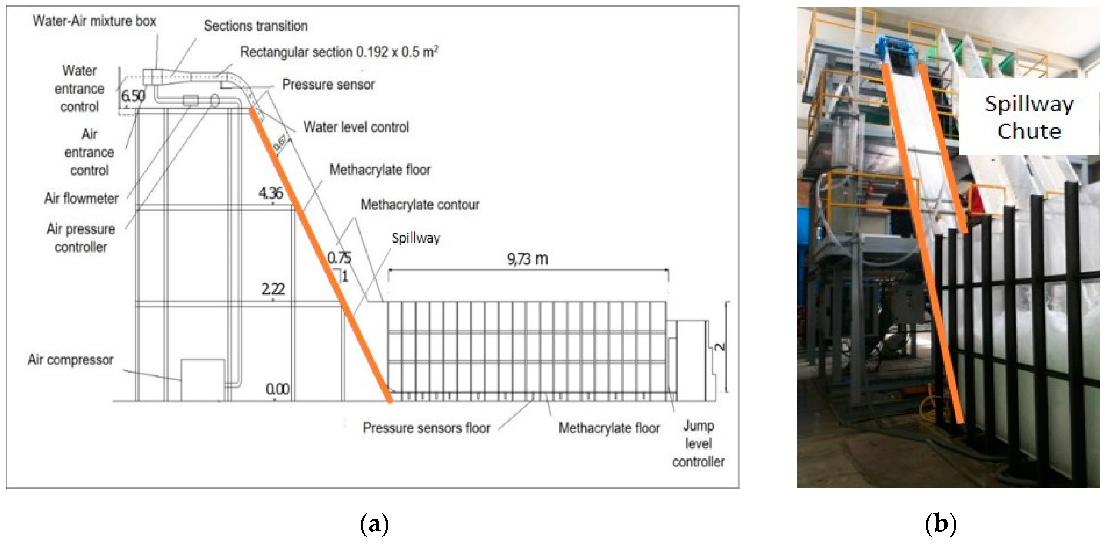
The installation built to reproduce the different flow scenarios consists of a spillway chute 6.5 m high and 0.5 m wide with a slope of 75%. This channel is followed by a horizontal stilling basin 10 m long and 2 m high, regulated by a control gate to confine the hydraulic jump. The objective of this element is to control the jump length and to recirculate excess water to the storage tank. Figure 1 shows a longitudinal section of the general system and includes a lateral view of the physical model in operation.
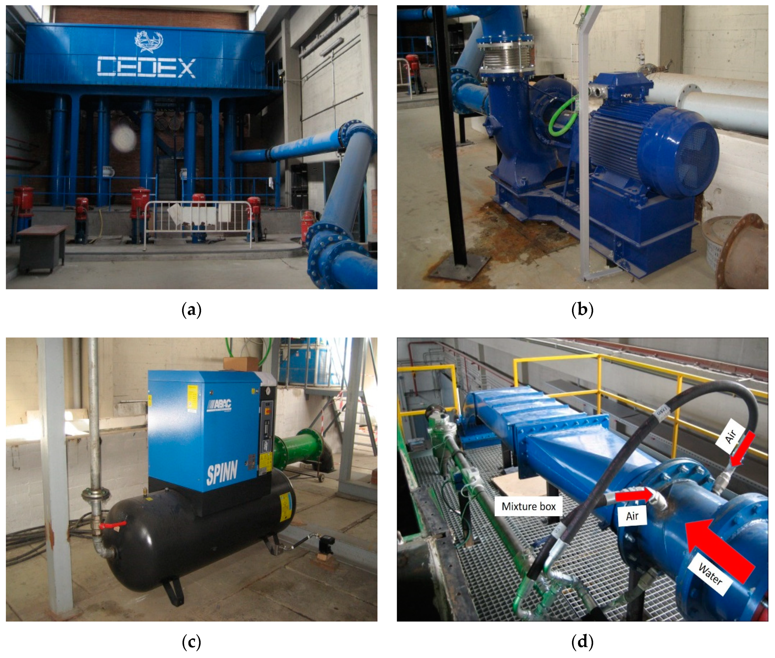
The system is equipped with a pump and air compressor to supply a maximum flow rate of 0.6 m3/s/m of water and 2000 L/s of air. Under these conditions, tested velocities vary between 5 and 7 m/s with Froude numbers between 5.5 and 6.5. The mixing of water and air takes place in a compartment just before the entrance to generate emulsionated flow. This process is very important for the analysis because the concentration of this intake flow is the initial condition of the experiment. Figure 2 shows all elements included in the physical model feeding. The channel intake is controlled by an adjustable gate in the upstream section. In this experimental study, an aperture of 0.08 m has been fixed for all tests (Figure 3b).
2.2. Control and Instrumental Devices
Water and air intake flows were regulated with two flowmeters before the mixture box. Pressure control was implemented in the air entrance section to improve the regulation capacity. The mixture box is equipped with a pressure sensor at the bottom to record the pressure measurements during the experimental analysis. These data are necessary to determine velocity evolution of the emulsionated flow (Figure 4).
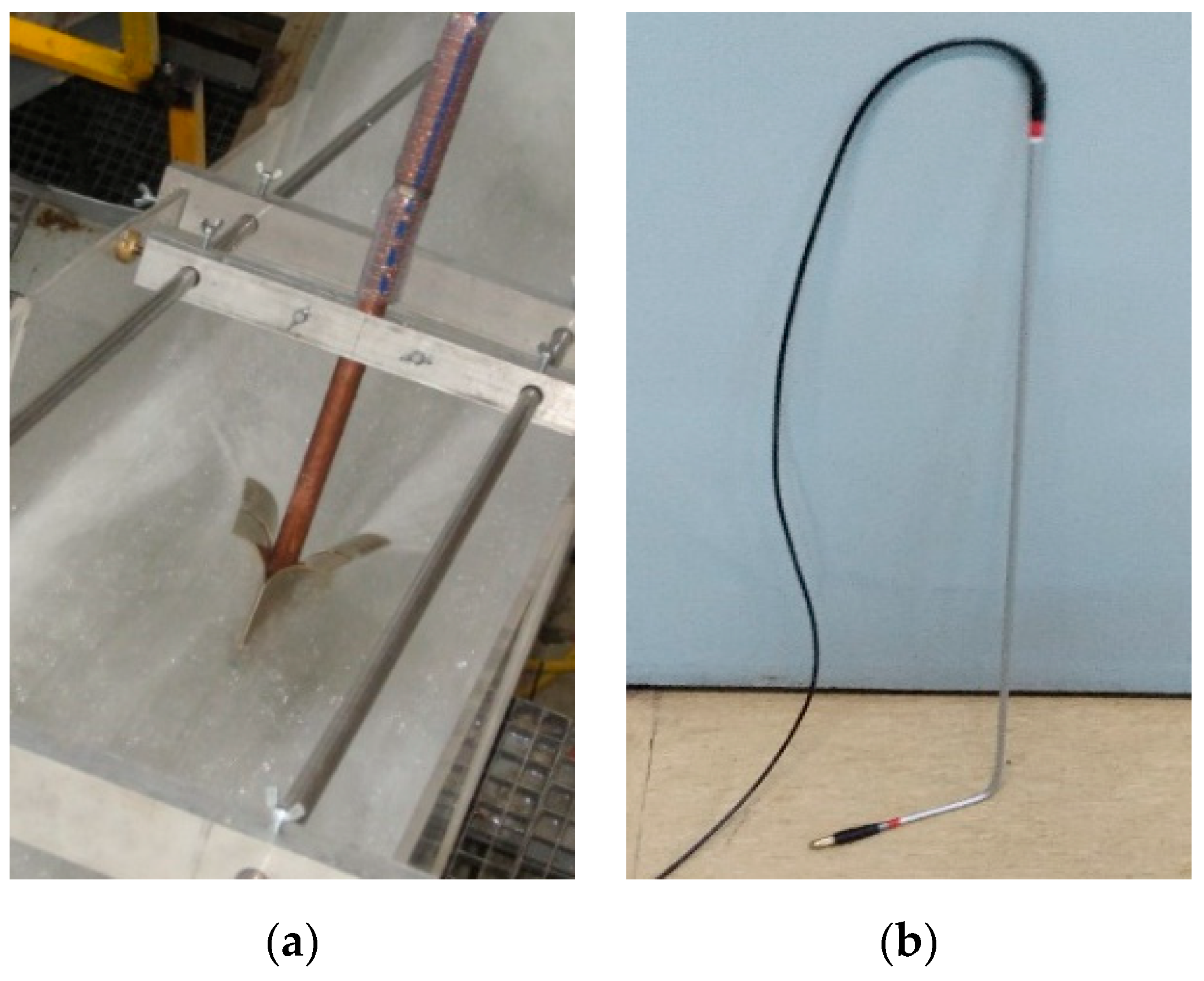
The second group of instrumental equipment is used to characterize the channel flow, measuring velocity and concentration profiles in the final section of the channel. A Pitot probe with a pressure sensor was used to measure the flow velocity. This sensor has a sampling frequency of 100 Hz and is connected to data acquisition software developed in CEDEX with LabVIEWTM 2010 (version 10.0 (32 bit), National Instruments, Austin, Texas, USA). Recording time in each test was 100 s. Post-processing was done considering manometric pressure head, atmospheric head and Pitot head. The total head is included in the energy Equation (1) to obtain the average velocity in every point.
where is the average velocity in the testing point, is the gravity acceleration and h is the specific head.
The measurement of concentration profiles was carried out with an Air Concentration Meter (ACM). This device was built by the Hydraulic Engineering Department of Universidad Politécnica de Cartagena (UPCT) and is based on a prototype developed in 1997 by the U.S. Department of the Interior Bureau of Reclamation [19] This experimental method was successfully applied by Cain, Wood and Chanson [20,21,22,23]. This probe measures air concentration in flowing water, detecting the air bubbles passing through the section by the changes in conductivity that take place when a bubble impinges on the probe tip. Analyzing the signal, it is possible to define two clear phases over time, water and air, and determine the concentration measurements. In this case, the acquisition frequency in all tests was 60 data/s and the recording time was set to 45 s. Figure 5 includes two pictures showing the Pitot and conductivity probes during the experimental phase.
2.3. Experimental Boundary Conditions
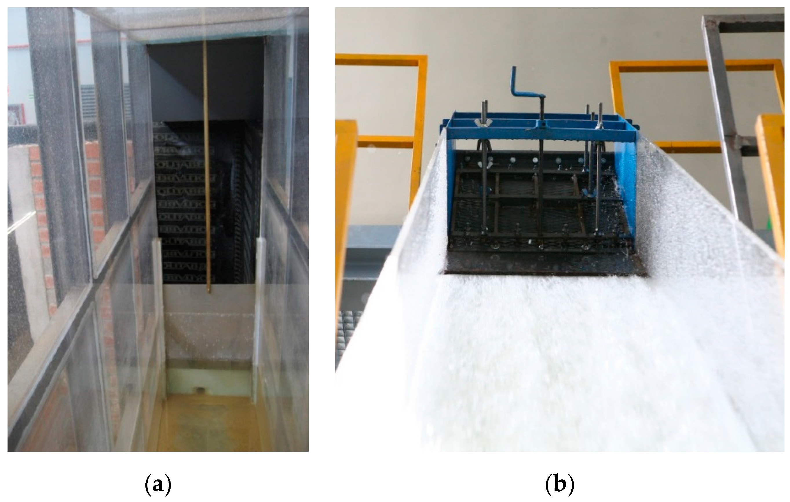
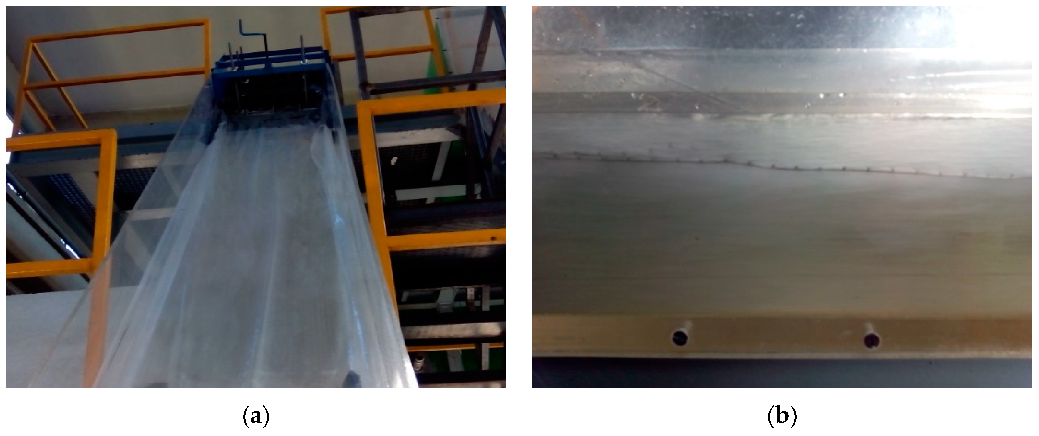
The real flow condition in the spillway must be fully turbulent. For this reason, a cover of metallic mesh was disposed along the top of the channel to increase turbulence. A flexible plastic cover was set over the channel as well, to reduce the air exchange between flow and atmosphere. Both materials are flexible and do not hinder free flow (Figure 6).
The plastic cover and metallic mesh will have influence in the velocity profile due to both elements increase the roughness at the surface and slow down the flow, moving the maximum velocity from the top flow to the low area of the flume.
2.4. Test Program
The twelve emulsionated flow scenarios analyzed in this research are summarized in Table 1, combining four water rates (Qw) with three intake airflows (Qa). With these data measured by the intake water and air flowmetres (Figure 4a,b)), and taking into account that gate opening has a fixed section 0.5 m wide and 0.08 m deep, it is possible to know the average velocity (VIn) and air concentration (CIn) at the intake channel. Moreover, a pressure sensor has been disposed below the mixture box (Figure 4d) to consider the air compressibility and correct the total mixture flow at the nozzle in atmospheric conditions, basic data to determine the real value of VIn.
All test recorded have placed at the axis of the channel section to reduce the effect of the sidewalls as much as possible.
3. Experimental Results
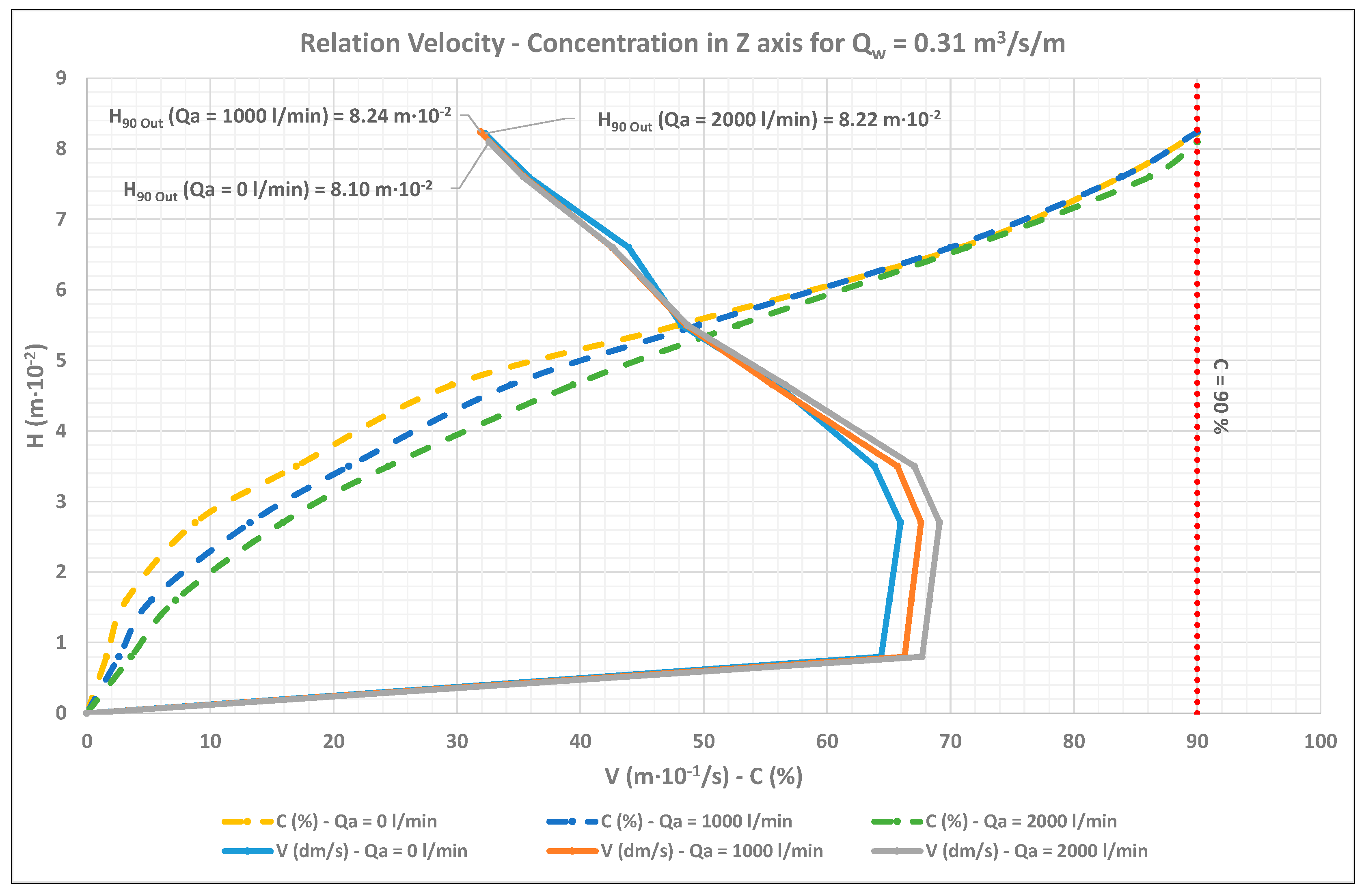
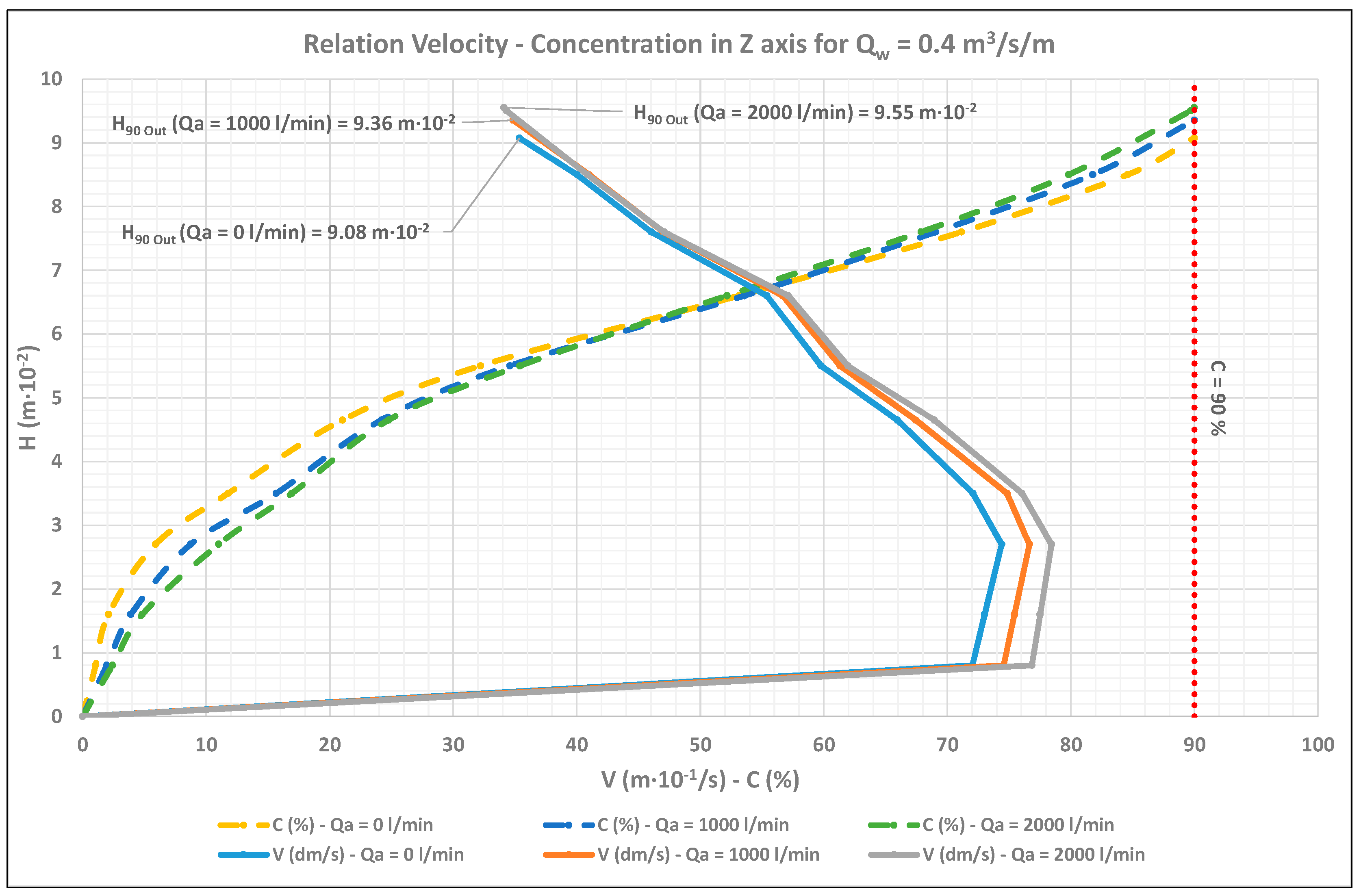
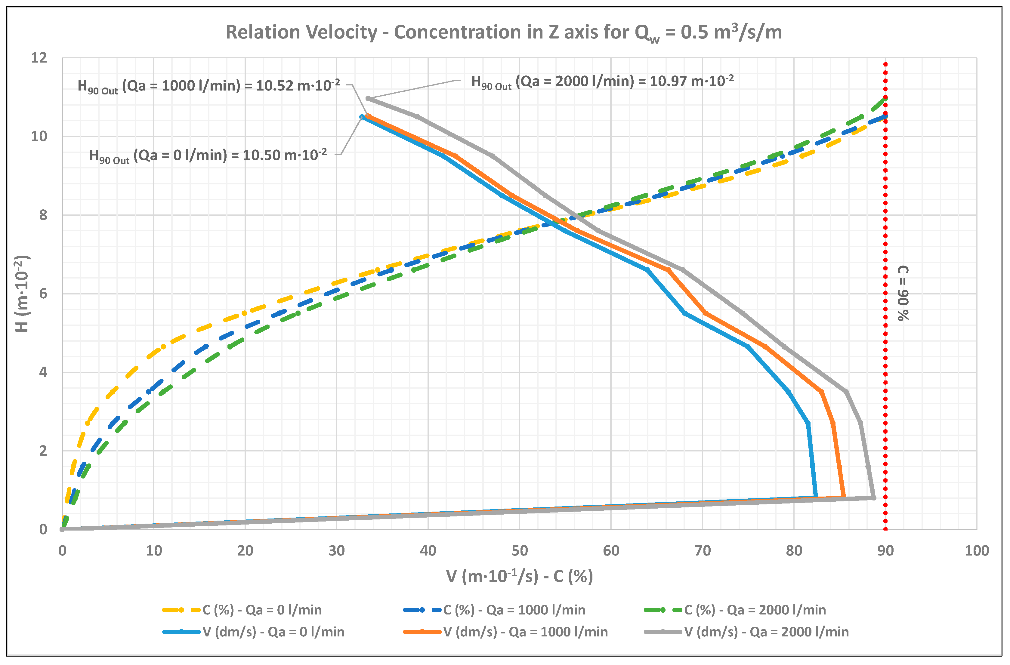
The velocity (VOut) and concentration (COut) profiles obtained during the experimental works are presented in Figure 7, Figure 8, Figure 9 and Figure 10. These values were measured in the axis of the channel, at 0.25 m of each side wall. Table 2 shows the average velocities, concentration values and depths at which concentration profile reaches 90% (H90 Out). This indicator is very common in the related scientific literature to set the free surface. Table 2 includes also the Froude, Reynolds and Weber numbers in the measurement section.
Figure 7 shows how flow velocity (VOut) increases as air concentration (COut) rises in the lower section of the channel for the test conducted with Qw = 0.31 m3/s/m. The strongest effect of air concentration on flow velocity was obtained on the first 4.5 cm from the bottom. Both variables were seen to increase an intake air flow rate (Qa) increased. The strongest effect was seen at 2.7 cm depth, where velocity changes from 0.66 m/s with 8.7% concentration to 0.69 m/s with 15.8 %. The H90 Out obtained in the three tests were similar with small variations of mm.
In the scenario corresponding to Qw = 0.4 m3/s/m (Figure 8), the observed tendency is similar to that of Figure 7. With a higher flow rate, the influence of aeration on the velocity profile extends to a depth of 5.5 cm. As in the previous test, the maximum velocity increase is observed at 2.7 cm depth, from 0.74 m/s with 5.9% air concentration to 0.78 m/s with 11%. H90 Out values also increase up to 1 cm more with respect to the previous scenario in all tests, with a maximum height of 9.55 cm in the test with Qa = 2000 L/min.
The third scenario (Figure 9) corresponds to tests with a water flow rate of Qw = 0.5 m3/s/m. In this scenario, the maximum velocity and air concentration variations are observed on the first 6.5 cm from the bottom. Velocity varies from 0.82 m/s with 1.2% air concentration to 0.88 m/s with 2.9% air concentration at a depth below 1.6 cm. The maximum H90 Out corresponds to the highest air flow rate and reaches almost 11 cm.
Figure 10 shows the final scenario results with the maximum flow rate of Qw =0.6 m3/s/m. In these tests, the major velocity variation is given also in the lower section, at 2.7 cm depth, with an increase from 0.9 m/s with 1.5% air concentration to 0.95 m/s with 2.6%. It is possible to appreciate the highest H90 Out in this scenario with the top value of 12.2 cm.
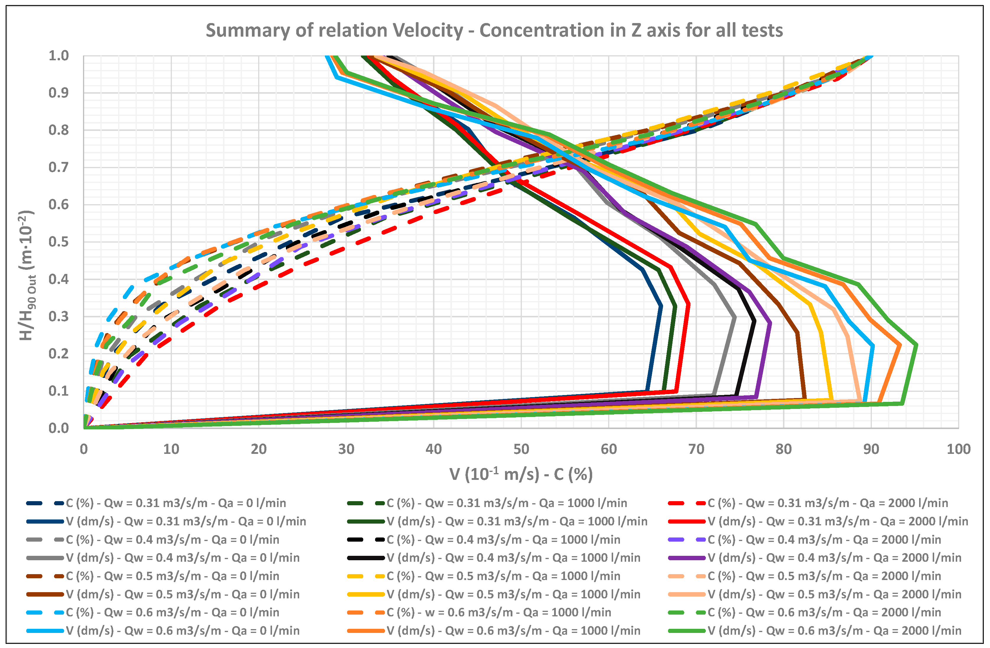
As a summary, Figure 11 shows the relation between velocity and air concentration profiles in all scenarios. To allow for comparisons, this representation shows a dimensionless Y axis where depth (H) is normalized by the values of H90 Out obtained in the tests. Analyzing Figure 11 and Table 2 we can appreciate the evolution of velocity profiles with the air concentration increase in all scenarios and tests, according to the water flow rate and aeration values. Results also show that H90 Out are very similar in scenarios with the same water flow rate, a factor which affects the evolution of Manning’s coefficient.
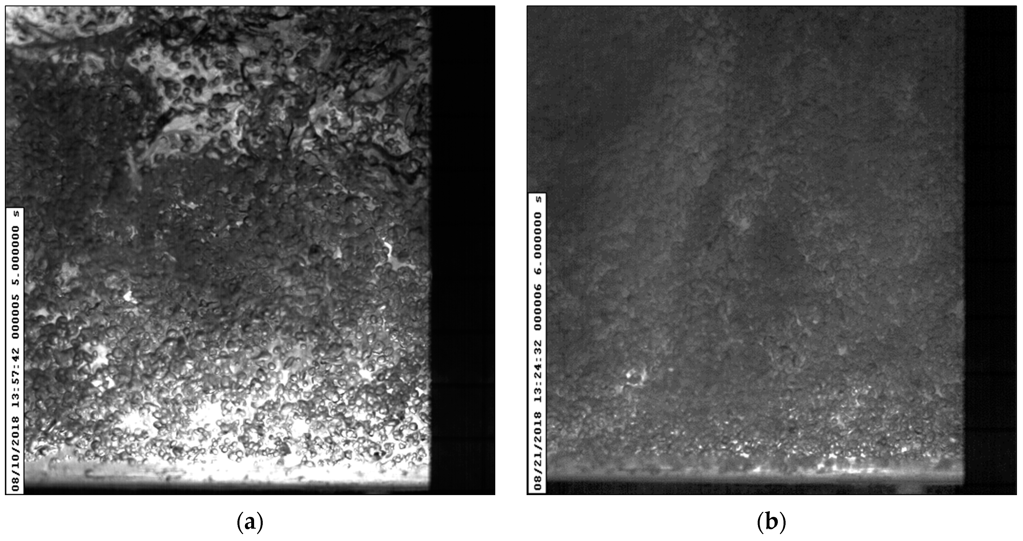
Other common effect in all scenarios is that concentration is zero at the bottom flume, due to there is no movement (VOut = 0 m/s) and flow cannot transport air bubbles. Figure 12 shows lateral views of this phenomena where velocity and concentration profiles have been obtained. These shots have been made with laser illumination and displays how the bubble density increases with the depth. Moreover, it is possible to see in the picture that concentration is zero (no bubbles) in the more illuminated areas, mainly located at the bottom flume.
4. Discussion
Aeration affects the energy dissipation mechanisms of open channel flows in different ways. First, Hinze [24] considers that aeration increases the viscous turbulent dissipation. This formulation refers to the reduction of the velocity profile with high concentration, but it is a theoretical proposal without empirical support.
Other authors, as Mateos, Wood and Chanson [25,26,27,28], consider the division and reunification of bubbles as the main factor over energy losses. They consider that shear stress between flow layers breaks the bubbles to later regroup each other in collision areas. This process has to exceed the surface tension of the air bubbles and generates energy dissipation by heat. Both formulations would be interesting during the analysis of the hydraulic jump, where turbulence effects are more important over the flow.
The third method is focused on analyzing energy dissipation by boundary friction and its application on open channel flow is most suitable. This proposal is different from the other two because both methodologies consider turbulence as the main effect of dissipation instead of roughness. Considering all the methods to evaluate this effect, Manning formulation (2) [29] has been chosen because it is well known and widely used in the hydraulic engineering area to determine the friction slope (If) based on a roughness coefficient (n), where V represents the average velocity and Rh the hydraulic radius.
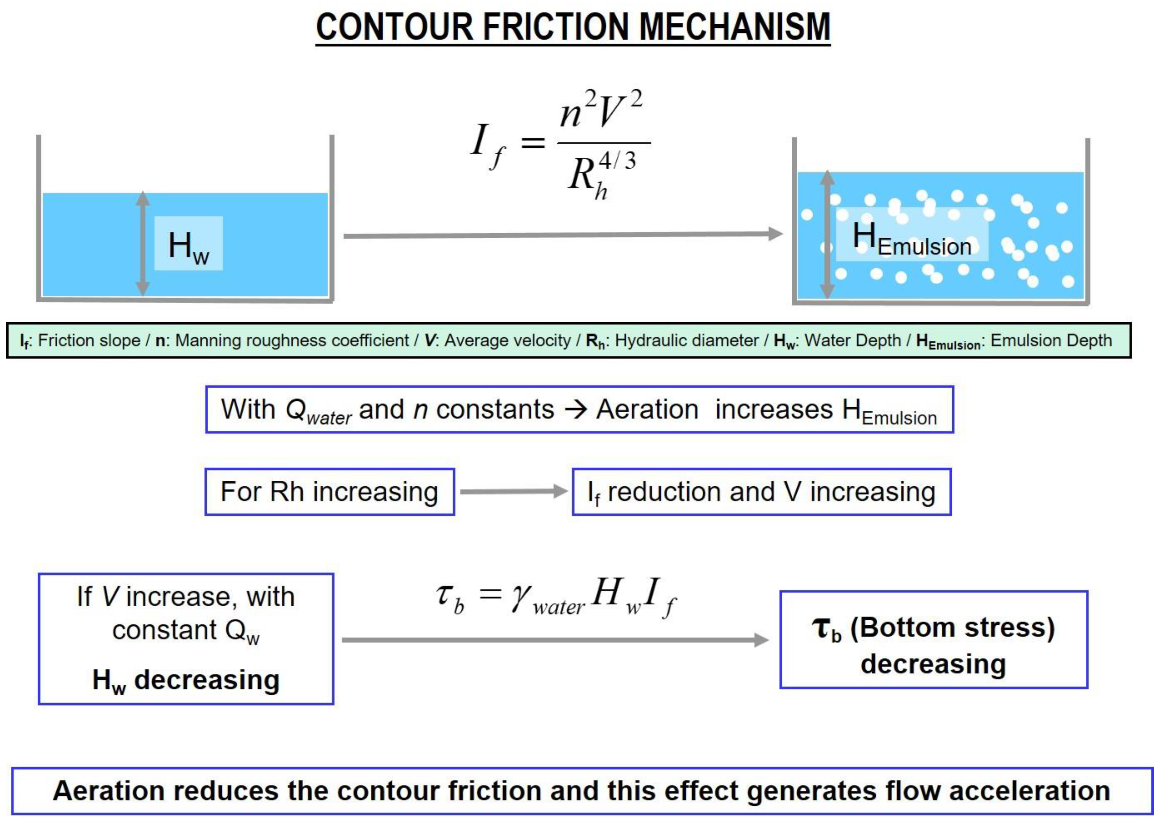
In our experimental case, we used Manning’s equation to analyze the energy dissipation due to boundary friction, which is prevailing in supercritical flows with low water depth and high velocity. In this sense, air bubbles imply an emulsion depth grow (HEmulsion) and the hydraulic radius (Rh) increases. Considering the last equation, this effect supposes a reduction of the friction slope (If) and velocity increase (V). Therefore, a velocity increase with water rate constant (Qw) generates a water depth decreasing (Hw), with the consequent reduction of the bottom stress (τb). Figure 13 shows the scheme of aeration influence in free surface flows and its effects over the boundary friction.
In general, the results obtained during the experimental phase show a velocity increase with the aeration growth for a constant water flow rate. Considering the velocity and air concentration profiles in the initial (VIn, CIn) and final (VOut, COut) sections of the channel, we calculated the characteristic average values of the flow in the spillway (VM, CM, H90 M) and also the friction slope of our test reach. Including these data in Manning’s equation, it is possible to determine the representative Manning’s roughness coefficient (n) and its reduction rate in % (∆n) with respect to the roughness without aeration. The Manning’s coefficients obtained in the middle of the spillway represent the final values for this prototype chute length, a factor which affects the roughness.
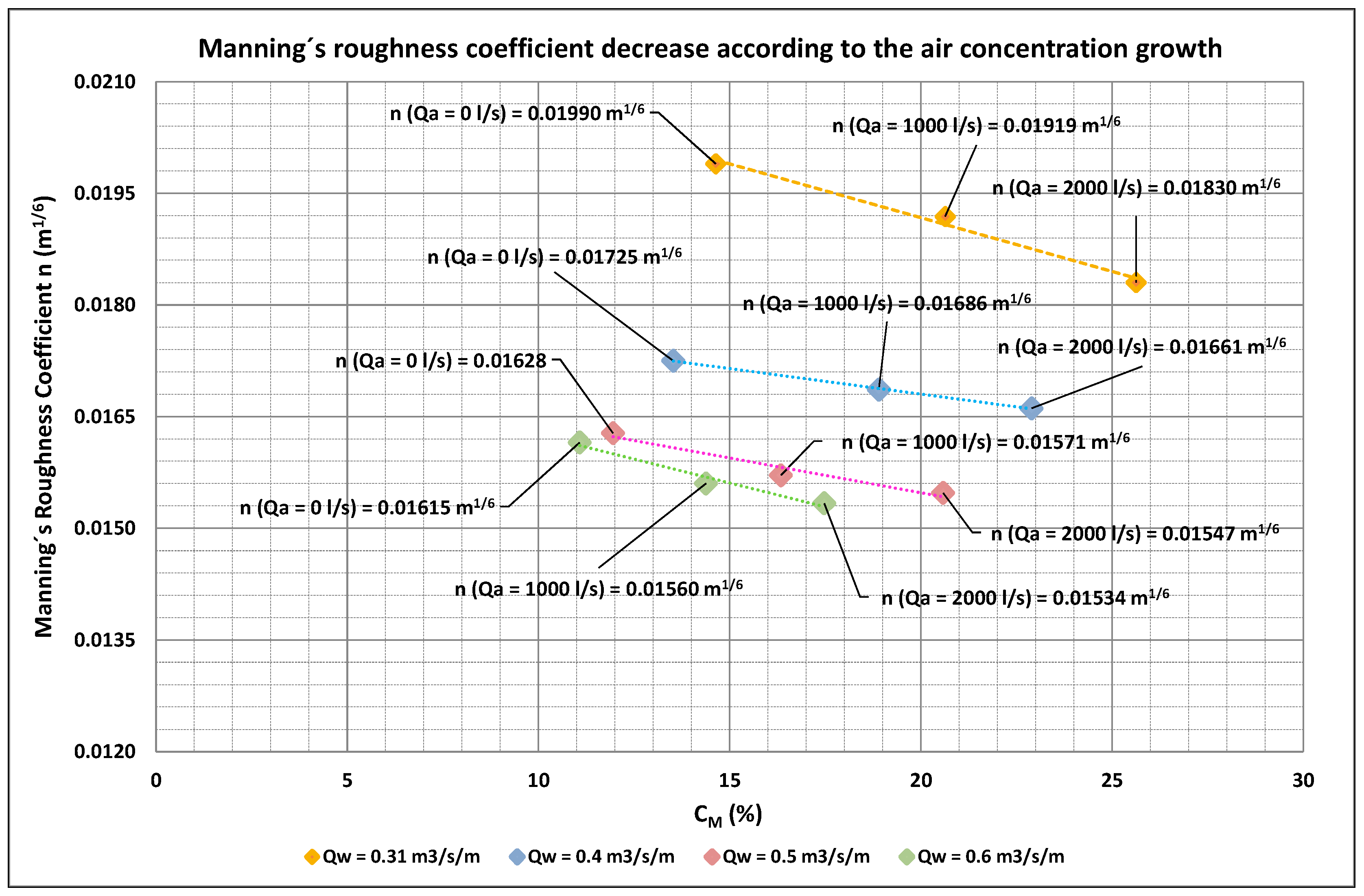
Table 3 includes the average values of the experimental results and Figure 13 relates the Manning’s roughness coefficient (n) with each concentration (CM) and demonstrates a roughness reduction with air concentration increase.
Analyzing the results shown in Figure 14, it is apparent that Manning’s coefficients decrease with increasing flow rates. This effect was expected, since the influence of boundary friction is lower with higher depths and it is a secondary factor which affects the Manning’s roughness constant. About this consideration, Chow [30] determines the material as the most important factor in the Manning’s coefficient but explains that other variables, as the stage and discharge or the suspended material, could influence the final value. The rate of reduction of roughness coefficient with concentration increase (line slope) is very similar in the four tests, with an average slope of 9 × 10⁻⁵ m1/6. With this singularity, it is possible to propose an equation to characterize the variation of the Manning’s roughness coefficient (n) as a function of the average air concentration (CM) in emulsionated flows Equation (3):
where n0 is the Manning’s coefficient with no air concentration in flow (CM = 0).
Experimental Reynolds and Weber numbers (Table 2) guarantee the representativeness of the results without scale effects. Performing a Froude similarity analysis and considering minimum numbers of Reynolds of 40,000 and Weber of 110, which make the effects of scale negligible, the representativeness of these results is guaranteed for prototypes with a geometric scale up to ten times larger than the model size.
5. Conclusions
This study is focused on the experimental analysis of aeration in supercritical and fully turbulent flow. The boundary conditions and large scale selected for the experimental process ensure the accuracy of the test. Obtained results show that aeration plays the main role in energy dissipation in open channel flows under these conditions. In our experimental results, with the same water flow rate, higher air concentration implies a velocity increase and, therefore, lower friction head losses. This reduction was quantified by means of the Manning’s coefficient (n). An original formulation was proposed to determine roughness (n) variation as a function of the average air concentration (CM) in emulsionated flows. Moreover, the dimensional analysis carried out in this study confirms that the representativeness of these results is guaranteed for prototypes with a geometric scale up to ten times larger than the model size.
Author Contributions
Conceptualization, J.J.R., D.L. and L.G.; Methodology, J.J.R., D.L., L.G. and R.D.; Instrumentation, R.H., J.J.R. and T.R.; Validation, J.J.R., R.D. and T.R.; Investigation, J.J.R. and D.L.; Analysis, discussion and results interpretation, J.J.R. and D.L.; Writing-Original Draft Preparation, J.J.R. and D.L.; Writing-Review & Editing, J.J.R., D.L. and L.G.
Funding
This research was supported by the Spanish Ministry of Economy in LS-EMULSION Project 2011–2014 (Grant No. 097326606-26606-4-11).
Acknowledgments
We wish to highlight the technical assistance of the Department of Hydraulic Engineering of UPCT (José María Carrillo, Paqui Marco and Luis Castillo) during the air concentration measurements and Ramón Gutierrez Serret (CEDEX) for his helpful and interesting bibliography about aeration in spillways. Their help is gratefully acknowledged.
Conflicts of Interest
The authors declare no conflict of interest.
References
- Straub, L.G.; Anderson, A.G. Experiments on self-aerated flow in open channels. J. Hydraul. Div. 1958, 84, 1–35. [Google Scholar]
- Chanson, H.; Toombes, L. Air-water flows down stepped chutes: Turbulence and flow structure observations. Int. J. Multiph. Flow 2002, 28, 1737–1761. [Google Scholar] [CrossRef]
- Valero, D. Modelación Hidráulico de Flujos Multifase en Grandes Presas. Aplicación al Diseño de Cuencos de Amortiguación. Master’s Thesis, Universidad Politécnica de Valencia, Valencia, Spain, 2015. (In Spanish). [Google Scholar]
- Chanson, H.; Chachereau, Y. Scale Effects Affecting Two-Phase Flow Properties in Hydraulic Jump with Small Inflow Froude Number. Exp. Therm. Fluid Sci. 2015, 45, 234–242. [Google Scholar] [CrossRef]
- Pfister, M.; Chanson, H. Two–phase air-water flows: Scale effects in physical modelling. J. Hydrodyn. 2014, 26, 291–298. [Google Scholar] [CrossRef]
- Boes, R.M. Scale effects in modelling two-phase stepped spillway flow. In Hydraulics of Stepped Spillways; Minor, H.E., Hager, W.H., Eds.; Balkema: Rotterdam, The Netherlands, 2000; pp. 53–60. [Google Scholar]
- Bombardelli, F.A.; Buscaglia, G.C.; Rehmann, C.R.; Rincón, L.E.; García, M.H. Modeling and scaling of aeration bubble plumes: A two–phase flow analysis. J. Hydraul. Res. 2016, 45, 617–630. [Google Scholar] [CrossRef]
- Gutiérrez Serret, J.R. Aireación en las Estructuras Hidráulicas de las Presas: Aplicación a Aliviaderos. Ph.D. Thesis, Universidad Politécnica de Madrid, Madrid, Spain, 1994. [Google Scholar]
- Moñino, A.; Riera, J. On the incipient aerated flow in chutes and spillways. J. Hydraul. Res. 2002, 40, 95–97. [Google Scholar] [CrossRef]
- Kramer, K.; Hager, W. Air Transport in chute flows. International. J. Multiph. Flow 2005, 31, 1181–1197. [Google Scholar] [CrossRef]
- Luna-Bahena, J.C.; Pozos-Estrada, O.; Ortiz-Martínez, V.M.; Gracia-Sánchez, J. Experimental Investigation of Artificial Aeration on a Smooth Spillway with a Crest Pier. Water 2018, 10, 1383. [Google Scholar] [CrossRef]
- Koen, J. Artificial Aeration on Stepped Spillways with Piers and Flares to Mitigate Cavitation Damage. Master’s Thesis, Stellenbosch University, Stellenbosch, South Africa, 2017. [Google Scholar]
- Bai, R.; Zhang, F.; Liu, S.; Wang, W. Air concentration and bubble characteristics downstream of a chute aerator. Int. J. Multiph. Flow 2016, 87, 156–166. [Google Scholar] [CrossRef]
- Bai, R.; Zhang, F.; Liu, S.; Wang, W. Experiments on Turbulence Intensity and Bubble Frequency in Self-Aerated Open Channel Flows. Water 2018, 10, 1201. [Google Scholar] [CrossRef]
- Cain, P. Measurements within Self-Aerated Flow on a Large Spillway. Ph.D. Thesis, University of Canterbury, Christchurch, New Zealand, 1978. [Google Scholar]
- Chanson, H. Self-aerated flows on chutes and super ways. J. Hydraul. Eng. 1993, 119, 220–243. [Google Scholar] [CrossRef]
- Pinto, N.L.S.; Neidert, S.; Ota, J. Aeration at high velocity flows—Part two. Int. Water Power Dam Constr. 1982, 34, 42–44. [Google Scholar]
- Felder, S.; Pfister, M. Comparative analyses of phase-detective intrusive probes in high-velocity air-water flows. Int. J. Multiph. Flow 2017, 90, 88–101. [Google Scholar] [CrossRef]
- Jacobs, M.L. Air Concentration Meter Electronics Package Manual; Project Notes 8450-98-01 1997; U.S. Department of the Interior Bureau of Reclamation: Denver, FL, USA, 1997.
- Cain, P.; Wood, I.R. Instrumentation for aerated flow on spillways. J. Hydraul. Div. 1981, 107, 1407–1424. [Google Scholar]
- Chanson, H. Study of air demand on spillway aerator. J. Fluid Eng. 1990, 112, 343–350. [Google Scholar] [CrossRef]
- Chanson, H. Air-water measurements with intrusive phase–detection probes: Can we improve their interpretation? J. Hydraul. Eng. 2002, 128, 252–255. [Google Scholar] [CrossRef]
- Chanson, H. A Study of Air Entrainment and Aeration Devices on a Spillway Model. Ph.D. Thesis, University of Canterbury, Christchurch, New Zealand, 1988. [Google Scholar]
- Hinze, J.O.; Milborn, H. Atomization of liquids by means of a rotating cup. J. Appl. Mech. 1950, 17, 145–153. [Google Scholar]
- Mateos, C. Aireación y Cavitación en Obras de Desagüe. Curso Sobre Comportamiento Hidráulico de las Estructuras de Desagües de Presa; CEDEX: Madrid, Spain, 1991. (In Spanish) [Google Scholar]
- Wood, I.R. Uniform region of self-aerated flow. J. Hydraul. Eng. 1983, 109, 447–461. [Google Scholar] [CrossRef]
- Wood, I.R. Air Entrainment in Free-Surface Flow: IAHR Hydraulic Structures Design Manuals 4; Balkema, A.A., Ed.; CRC Press: Rotterdam, The Netherlands, 1991. [Google Scholar]
- Chanson, H. Air Entrainment in Chutes and Spillways; Research Report No. CE 133 1992; Department of Civil Engineering of Queensland: St. Lucia, Australia, 1992. [Google Scholar]
- Manning, R. On the flow of water in open channels and pipes. Inst. Civ. Eng. Irel. 1891, 20, 161–207. [Google Scholar]
- Chow, V.T. Open-Channel Hydraulics; Mc Graw-Hill Book Company: New York, NY, USA, 1959; pp. 101–108. [Google Scholar]
Figure 1.
Design and characteristics of the physical model with spillway limits (orange color): (a) Model longitudinal section with materials and all the elements needed to establish the initial and boundary conditions and to reproduce the flow scenarios; (b) Lateral view of the spillway chute and stilling basin with the hydraulic jump.

Figure 2.
Water and air supply equipment: (a) Water gauger; (b) Water pump; (c) Air compressor; (d) Air-water mixture box.
Figure 2.
Water and air supply equipment: (a) Water gauger; (b) Water pump; (c) Air compressor; (d) Air-water mixture box.

Figure 3.
Initial and boundary conditions in the physical model: (a) Intake flow gate located at the entrance of the spillway chute; (b) Regulation gate to control the still basin.
Figure 3.
Initial and boundary conditions in the physical model: (a) Intake flow gate located at the entrance of the spillway chute; (b) Regulation gate to control the still basin.

Figure 4.
Control devices: (a) Water electromagnetic flowmeter; (b) Air flowmeter; (c) Air pressure control; (d) Atmospheric pressure sensor in mixture box.
Figure 4.
Control devices: (a) Water electromagnetic flowmeter; (b) Air flowmeter; (c) Air pressure control; (d) Atmospheric pressure sensor in mixture box.

Figure 5.
Velocity and concentration data collection: (a) Pitot probe during the velocity measurement process; (b) view of the Air Concentration Meter probe used in the concentration measurement process.
Figure 5.
Velocity and concentration data collection: (a) Pitot probe during the velocity measurement process; (b) view of the Air Concentration Meter probe used in the concentration measurement process.

Figure 6.
Boundary conditions over the flow surface during the experimental analysis: (a) Plastic cover to reduce air exchange between flow and atmosphere; (b) Effects of the metallic mesh and plastic cover over the flow in the test.
Figure 6.
Boundary conditions over the flow surface during the experimental analysis: (a) Plastic cover to reduce air exchange between flow and atmosphere; (b) Effects of the metallic mesh and plastic cover over the flow in the test.

Figure 7.
Relation between depth (H) and velocity (V)—Concentration (C) profiles in scenario 1 (Qw = 0.31 m3/s/m).
Figure 7.
Relation between depth (H) and velocity (V)—Concentration (C) profiles in scenario 1 (Qw = 0.31 m3/s/m).

Figure 8.
Relation between depth (H) and velocity (V)—Concentration (C) profiles in scenario 2 (Qw = 0.4 m3/s/m).
Figure 8.
Relation between depth (H) and velocity (V)—Concentration (C) profiles in scenario 2 (Qw = 0.4 m3/s/m).

Figure 9.
Relation between depth (H) and velocity (V)—Concentration (C) profiles in scenario 3 (Qw = 0.5 m3/s/m).
Figure 9.
Relation between depth (H) and velocity (V)—Concentration (C) profiles in scenario 3 (Qw = 0.5 m3/s/m).

Figure 10.
Relation between depth (H) and velocity (V)—Concentration (C) profiles in scenario 4 (Qw = 0.6 m3/s/m).
Figure 10.
Relation between depth (H) and velocity (V)—Concentration (C) profiles in scenario 4 (Qw = 0.6 m3/s/m).

Figure 11.
Summary of relations between velocity and concentration profiles in all scenarios.

Figure 12.
Lateral view of different scenarios in the measurement section: (a) Scenario with Qw = 0.4 m3/s/m and Qa = 0 L /s; (b) Scenario with Qw = 0.6 m3/s/m and Qa = 2500 L/s.
Figure 12.
Lateral view of different scenarios in the measurement section: (a) Scenario with Qw = 0.4 m3/s/m and Qa = 0 L /s; (b) Scenario with Qw = 0.6 m3/s/m and Qa = 2500 L/s.

Figure 13.
Scheme of the aeration effects over the boundary friction.

Figure 14.
The relation between Manning’s roughness coefficient (n) and average air concentration (CM) for all scenarios.
Figure 14.
The relation between Manning’s roughness coefficient (n) and average air concentration (CM) for all scenarios.


Table 1.
Experimental scenarios with average velocity and air concentration at the intake channel.
| Scenario | Qw (m3/s/m) | Qa (L/min) | VIn (m/s) | CIn (%) |
|---|---|---|---|---|
| 1.1 | 0.31 (155 L/s) | 0 | 3.88 | 0 |
| 1.2 | 1000 | 4.30 | 9.98 | |
| 1.3 | 2000 | 4.74 | 18.23 | |
| 2.1 | 0.4 (200 L/s) | 0 | 5.00 | 0 |
| 2.2 | 1000 | 5.45 | 8.26 | |
| 2.3 | 2000 | 5.91 | 15.43 | |
| 3.1 | 0 | 6.25 | 0 | |
| 3.2 | 0.5 (250 L/s) | 1000 | 6.72 | 6.97 |
| 3.3 | 2000 | 7.21 | 13.27 | |
| 4.1 | 0 | 7.50 | 0 | |
| 4.2 | 0.6 (300 L/s) | 1000 | 8.00 | 6.30 |
| 4.3 | 2000 | 8.53 | 12.06 |
Table 2.
Average velocity, concentration and H90 values at the channel exit.
| Scenario | VOut (m/s) | COut (%) | H90 Out (m·10−2) | Fr | Re·106 | We |
|---|---|---|---|---|---|---|
| 1.1 | 5.19 | 29.28 | 8.2 | 5.78 | 1.24 | 30,371 |
| 1.2 | 5.24 | 31.30 | 8.2 | 5.83 | 1.24 | 31,074 |
| 1.3 | 5.35 | 33.03 | 8.1 | 6.01 | 1.24 | 31,884 |
| 2.1 | 5.88 | 27.05 | 9.1 | 6.23 | 1.60 | 43,120 |
| 2.2 | 5.98 | 29.54 | 9.3 | 6.24 | 1.60 | 45,940 |
| 2.3 | 6.03 | 30.37 | 9.6 | 6.22 | 1.60 | 47,640 |
| 3.1 | 6.32 | 23.90 | 10.5 | 6.22 | 2.00 | 57,516 |
| 3.2 | 6.52 | 25.71 | 10.5 | 6.42 | 2.00 | 61,402 |
| 3.3 | 6.69 | 27.89 | 11.0 | 6.45 | 2.00 | 67,313 |
| 4.1 | 6.59 | 22.16 | 12.2 | 6.03 | 2.40 | 72,866 |
| 4.2 | 6.81 | 22.46 | 12.0 | 6.27 | 2.40 | 76,737 |
| 4.3 | 6.95 | 22.88 | 12.0 | 6.39 | 2.40 | 79,859 |
Table 3.
Average velocity, concentration, H90 and n value at the middle section of the channel.
| Scenario | VM (m/s) | CM (%) | H90 M (m·10−2) | n | ∆n (%) |
|---|---|---|---|---|---|
| 1.1 | 4.53 | 14.64 | 8.1 | 0.0199 | 9.81 |
| 1.2 | 4.77 | 20.64 | 8.1 | 0.0192 | 13.02 |
| 1.3 | 5.05 | 25.63 | 8.0 | 0.0183 | 17.05 |
| 2.1 | 5.44 | 13.52 | 8.5 | 0.0173 | 5.06 |
| 2.2 | 5.71 | 18.90 | 8.7 | 0.0169 | 7.19 |
| 2.3 | 5.97 | 22.90 | 8.8 | 0.0166 | 8.58 |
| 3.1 | 6.28 | 11.95 | 9.2 | 0.0163 | 5.58 |
| 3.2 | 6.62 | 16.34 | 9.3 | 0.0157 | 8.86 |
| 3.3 | 6.95 | 20.58 | 9.5 | 0.0155 | 10.24 |
| 4.1 | 7.05 | 11.08 | 10.1 | 0.0162 | 7.86 |
| 4.2 | 7.41 | 14.38 | 10.0 | 0.0156 | 11.00 |
| 4.3 | 7.74 | 17.47 | 10.0 | 0.0153 | 12.52 |
© 2019 by the authors. Licensee MDPI, Basel, Switzerland. This article is an open access article distributed under the terms and conditions of the Creative Commons Attribution (CC BY) license (http://creativecommons.org/licenses/by/4.0/).
Share and Cite
MDPI and ACS Style
Rebollo, J.J.; López, D.; Garrote, L.; Ramos, T.; Díaz, R.; Herrero, R. Experimental Analysis of the Influence of Aeration in the Energy Dissipation of Supercritical Channel Flows. Water 2019, 11, 576. https://doi.org/10.3390/w11030576
AMA Style
Rebollo JJ, López D, Garrote L, Ramos T, Díaz R, Herrero R. Experimental Analysis of the Influence of Aeration in the Energy Dissipation of Supercritical Channel Flows. Water. 2019; 11(3):576. https://doi.org/10.3390/w11030576
Chicago/Turabian StyleRebollo, Juan José, David López, Luis Garrote, Tamara Ramos, Rubén Díaz, and Ricardo Herrero. 2019. "Experimental Analysis of the Influence of Aeration in the Energy Dissipation of Supercritical Channel Flows" Water 11, no. 3: 576. https://doi.org/10.3390/w11030576
Note that from the first issue of 2016, this journal uses article numbers instead of page numbers. See further details here.