
Fully Coupled Vibrations of Cable-Harnessed Beams with a Non-Periodic Wrapping Pattern


1
Department of Mechanical and Mechatronics Engineering, University of Waterloo, Waterloo, ON N2L 3G1, Canada
2
Application Engineering, Maplesoft Inc., Waterloo, ON N2V 1K8, Canada
*
Authors to whom correspondence should be addressed.
Vibration 2022, 5(2), 238-263; https://doi.org/10.3390/vibration5020015
Submission received: 23 December 2021
/
Revised: 8 March 2022
/
Accepted: 5 April 2022
/
Published: 13 April 2022
Abstract
:Power- and signal- cable attachments have a significant impact on the vibrations of space structures. Recent works show the importance of having an analytical model to gain physical insight into the influence of cabling on the dynamics of host structures. The models in the literature focus mainly on pure bending vibrations and ignore the effect of coupling between different coordinates. Recently, the authors demonstrated the importance of modeling the coupling effects in cable-harnessed (CH) beams with straight and periodic wrapping patterns. In real-life situations, the cable attachment patterns are mostly non-periodic, and the cables are also attached to host structures that consist of a combination of several harness elements of same (homogenous) or different (non-homogenous) material properties. Hence, the fully coupled vibration model developed in this article is the first to analyze the vibrations of homogenous and non-homogenous CH beams with non-periodic wrapping patterns. The Frequency Response Functions (FRFs) of the developed model are compared with experiment FRFs in the case of the homogenous non-periodic wrapping pattern. The study shows that the coupling effects are pronounced in non-periodic wrapped CH beams, and the advantage of developing the coupled model over the decoupled model is shown through experimental validation.
1. Introduction
Research on the influence of cabling on the dynamics of space structures has received increased attention in recent years. Power- and signal- cable harnesses account for a significant percentage of the total mass of these structures [1]. Hence, the cable harness is found to alter the vibratory behavior of space structures. Additionally, it is difficult to experimentally determine the effect of cable attachments before the structure is launched. As a result, it was deemed important to accurately model these effects, and the U.S. Air Force Research Laboratory (U.S. AFRL) [1,2,3] was the first research group to study the vibrations of cable-harnessed (CH) structures.
The goal of the U.S. AFRL included development of the Finite Element Model (FEM) and experimental techniques to study the vibration characteristics of CH structures with straight cable patterns, with a focus on decoupled bending vibrations. Babuska et al. [1] developed experimentally validated FEM models to study the stiffness effect due to straight cable attachments on the CH beams. Robertson et al. [2] and Goodding et al. [3] developed experimental techniques such as cable attachment to host structures and continuous vibration models, respectively, to study the decoupled bending vibrations in beams attached with straight cables. Coombs et al. [4] further expanded the research to analyze the vibrations of cable-harnessed panels using experiments. Kauffmann et al. [5,6] experimentally characterized the damping effects in standalone thick cables. The mentioned studies conclude that further analytical modeling is essential to properly understand the dynamic effects of cabling. Later, Spak et al. [7,8] developed analytical models and incorporated stiffness and damping effects in structures with straight cable patterns. The Distributed Transfer Function Method (DTFM) was also developed to accurately study the dissipation effect in CH structures across several bending modes. The works described so far further emphasize the importance of developing an analytical model to gain a physical understanding of the vibrations of CH structures. The primary purpose of formulating an accurate analytical model is to design high-fidelity control systems for the space structures. Additionally, an analytical model helps to obtain better physical insight into system dynamics when compared to the standard practice of using commercially available FEM models in the industry.
The mathematical models used by the U.S. AFRL consider the straight cable attachment pattern. However, the cables can be attached in a more complex manner, for example, they can be wrapped around the structure. To understand the dynamics of such structures, our research group developed low-order analytical models by considering periodic cable harnessing patterns. Martin and Salehian [9,10] developed experimentally validated models to analyze the pure bending vibrations of periodic CH beams. They assumed that the cable had pre-tension and that it applied a pre-compressive force on the host beam. Higher-order strain-displacement relations were developed, [9], and the model was experimentally validated [10]. The models developed by Martin and Salehian [9,10], however, ignored damping due to the cables, which was later introduced by Agrawal and Salehian [11], primarily for predicting accurate amplitudes in the frequency response in the resonant frequency region. In the studies described so far [9,10,11], the models ignore the effect of coordinate coupling.
Yerrapragada and Salehian [12,13] developed an experimentally validated vibration model that considers coordinate coupling in CH beams with straight and periodic wrapping patterns. It was reported that as the cabling on the beam increases, the coupling effect becomes significant and cannot be ignored. Earlier, in the experimental investigations by Martin and Salehian [10], the coupling effects were negligible due to the lower number of cables harnessed in their study. These studies primarily considered periodic wrapping patterns to study the dynamics of CH beams. In one of their recent works, Martin and Salehian [14] studied the decoupled vibrations of CH beams with a non-periodic wrapping pattern. The study was confined only to vibrations in the out-of-plane bending (OP) coordinate of the beam structure. It must be noted that wrapping the cable in a non-periodic manner is a more general case related to space structure cable-harnessing [1,4,7] than the straight and periodic wrapping cases.
In the above-mentioned studies, small vibration levels are considered. For small amplitudes, the linear assumptions hold true, and it can be assumed that the cable stays in contact in host structure. The CH structures for small vibration levels are analogous to the composite structures. In composites, the fibers are often aligned in different patterns in the matrix, depending on the directional strength requirements. Several vibration studies [15,16,17] on composite beams consider the coupling between the out-of-plane bending, torsion, and in-plane bending coordinates. Coupling in composites is due to the fibers’ material and their orientation. Ref. [18] demonstrates the significant differences in natural frequencies of coupled and decoupled models in composite beam vibrations. In practical CH structures related to space applications, the cables can be wrapped around the host structure in several periodic and non-periodic configurations. So, different elements of the CH structure can have different combinations of cable- and host-structure properties (geometric and material properties). However, in the studies published so far, the analytical models are limited to homogenous host structures in a periodic pattern. The investigation of coupling effects of CH beams with non-periodic pattern is an existing gap in the literature.
In the current paper, a generalized analytical model is developed to analyze the fully coupled vibrations of CH beams with both homogenous and non-homogenous host structures wherein the cable is harnessed in a non-periodic manner. The pattern consists of multiple fundamental elements, each comprising a diagonal cable section and a lumped-mass cable section. In structures with more cables and fewer fundamental elements, the effect of coupling will be more significant [13,19]. The coupling also depends on the material properties of the host structure and the cable. The coupling effects in the non-homogenous structures are found to be higher when compared to the homogenous structures for the considered different material properties in each fundamental element. Consideration of the combination of the coupling effects, non-periodic wrapping pattern, and non-homogenous host structures makes the developed model more generic for studying the vibrations of CH beams. Due to multiple non-periodic fundamental elements, the energy-equivalent homogenization technique developed by Martin and Salehian [9] for periodic CH beams cannot be used. Continuity conditions are applied at the interface of each fundamental element involving all the coordinates of motion to make the problem tractable. Finally, for homogenous host structures, the results obtained from the theoretical studies are validated using experiments.
In Section 2, the coupled PDEs for the CH beam with a non-periodic cable attachment pattern are presented. In Section 3, theoretical analysis is performed on both homogenous and non-homogenous CH beams. The FRF characteristics of the developed model are compared and analyzed with respect to the experiment FRF in the case of a non-periodic wrapped CH beam with a homogenous host structure. Experimental mode shapes for the torsion and in-plane bending (IP) modes are also presented to confirm their identities.
2. Mathematical Modeling
In Section 2, the CH beam system is described. First, the strain energies and kinetic energies (SE and KE) are obtained from the stress and strain tensors. Second, fully coupled PDEs are presented along with the procedure to obtain the natural frequencies.
2.1. Derivation of Strain and Kinetic Energies
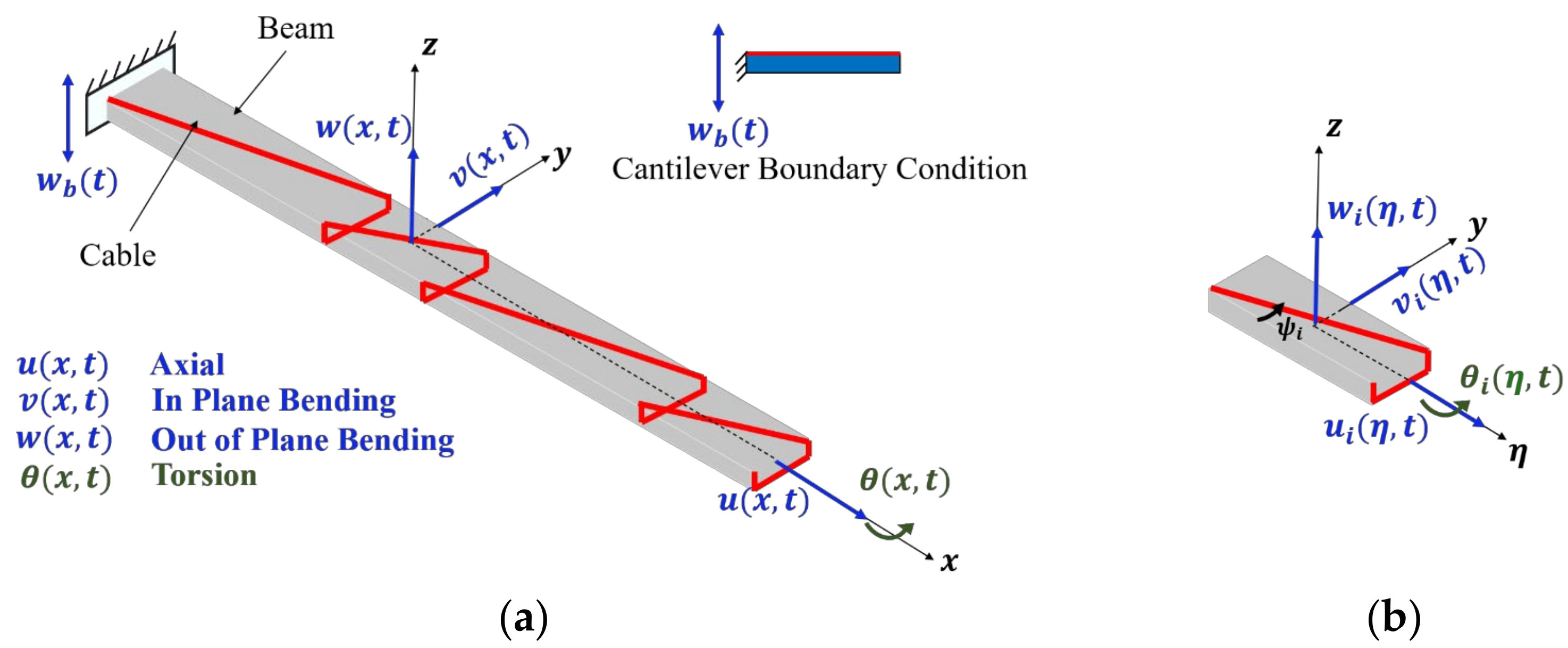
The CH beam with the non-periodic cable attachment is shown in Figure 1a in the global coordinate system . A fundamental wrapping element of the full system is shown in Figure 1b along with the local coordinate system . Each wrapping element contains a diagonal cable part and a lumped-mass cable part at the end of each fundamental element. The wrapping angle is different in each element. This represents a more realistic case of cable attachment pattern than the periodic wrapping patterns previously studied by the authors [19]. The system shown in Figure 1b represents a homogenous cable harnessed structure where each fundamental element has the same material properties for the beam and cable. For the most generalized case, each fundamental of the host structure and cable have different material properties, and they are referred to as cable-harnessed structures with a non-homogenous host structure and non-homogenous cables. The following derivations are performed for the most generalized case.
The coordinates are defined as axial , in-plane bending (IP) , out-of-plane bending (OP) , and torsion . The displacements of an ith element are denoted by and (refer to Figure 1b). The model assumptions are as follows [13,20]:
- The cable will be in pre-tension during harnessing and remains in tension during structural vibrations.
- The cable pre-tension, T, results in a pre-compressive load on the beam.
- The cable remains attached to the beam during vibrations; friction between the beam and cable is ignored.
- The cable strains are the same as that of the top fiber of the beam.
The second-order displacement field involving all the degrees of freedom using Euler–Bernoulli theory is shown in Equation (1) [9,21]:
, and are the displacement components for all points of the beam of the given coordinates. To develop a fully coupled vibration model, consideration of all the coordinates in the displacement field is important. . The Green–Lagrange strain tensor is given by Equations (2)–(4), respectively [9,21,22]:
where is the normal strain and and are the shear strains. The equations for the displacement field, the strain tensor, and the stress–strain relationship are used to arrive at the SE and KE of a fundamental element of the CH beam, employing the EB theory assumptions (Equations (5) and (6)).
Here, superscript . and are the areas of cross-section of the beam and the cable, respectively. and are the Young’s modulus of the beam and the cable for the fundamental element, respectively. and are the densities of the beam and the cable for the fundamental element, respectively. is the shear modulus of the beam for the fundamental element. and are the width and thickness of the beam. The fundamental element has the length and the wrapping angle is , where and ; are the strains experienced by the beam. The SE contribution in a fundamental element due to the cable () and the beam () are shown in Equations (7) and (8), respectively:
Substituting the strain tensor Equations (2)–(4) in Equations (7) and (8) and neglecting terms with an order , we obtain the SE due to the cable and the beam, and the intermediate derivation step is shown in Appendix A Equations (A1) and (A2). The terms of strain energy expression with an order often result in non-linearities in the vibration model. Such higher-order terms are neglected, as the goal of this study is to investigate the linear vibrations. Our early study [9] on linear decoupled vibration of cable-harnessed structures emphasized the importance of using second-order displacement along with a Green–Lagrange strain tensor to obtain accurate frequency responses with respect to the experiment. Hence, a Green–Lagrange strain tensor is also used in this study. The total SE in an element can be obtained using . The final forms of the SE and KE in the fundamental element are shown in Equations (9) and (10):
where superscript and represent the SE and KE coefficient of the fundamental element where is an index. The constant terms in Appendix A Equations (A1) and (A2) do not play any part in the vibration analysis, as the constant terms vanish when Hamilton’s principle is applied. The constant terms are not shown in the final strain energy. The terms , and in Appendix A Equation (A1) result in non-homogenous boundary conditions in the governing equations of motion, as shown in the previous works by our research group [9,10]. An appropriate choice of time-independent solution will convert the non-homogenous boundary condition into a homogenous one. The eigenvalue problem to obtain the natural frequencies remains unaffected due to this operation [9,10] and hence, those decoupled terms are omitted in the final strain energy expression, Equation (9). The coefficients of Equations (9) and (10) are presented in Equation (11). The developed model for the non-homogenous structure can be reduced to that of the homogenous structure by considering the same material properties for the beam (,) and the cable (,) across all the fundamental elements.
and . . . In Equations (9) and (10), it is observed that the coefficients , and are spatially variable. This would make it impossible to obtain an analytical solution, using the coupled PDEs, that will be obtained from the exact strain and kinetic energies of Equations (9) and (10). The variable coefficients in Equations (9) and (10) are averaged over the length of the element. The resulting SE and KE for a given element are shown in Equations (12) and (13):
In the case of non-periodic CH beams in this paper, the wrapping angle and, in some cases, the material properties vary from one element to the other. A homogenization approach developed by the authors before [19] cannot be applied in this case. As a result, continuity conditions at the interface of the two elements must be applied.
2.2. Solution to the Coupled Partial Differential Equations
Once the SE and KE of the element are obtained as described in Section 2.1, the energies of the CH system can be obtained as shown in Equations (A4) and (A5). Then, the Extended Hamilton’s principle [23,24] is applied to the entire system and is used to derive the fully coupled PDEs for the CH beam. The boundary conditions and continuity conditions at the interface are also derived, and are shown in Appendix A Equation (A7). From these equations, the eigenvalue problem is formulated. The constant-coefficient coupled PDEs are shown in Equations (14a)–(14d). The procedure to formulate the eigenvalue problem of these coupled PDE types is shown in our previous work [12,13].
where and represent the SE and KE coefficient of the fundamental element. The final averaged coefficients are shown in Appendix A Equation (A3). The cable strain is evaluated at . The solution form of PDEs in Equations (14a)–(14d) is assumed to be Equation (15):
where .
Substituting Equation (15) into Equations (14a)–(14d), we obtain:
The fixed end boundary conditions are shown in Equation (17):
The free end boundary conditions are shown in Equations (18a)–(18f):
In Equations (18a)–(18f), the lumped-mass expressions are shown in Appendix A Equation (A6). The continuity conditions for the coupled model at the interface, —including the effect of all the coordinates, where the displacement, slope, moment, and shear are assumed to be continuous—are shown in Appendix A Equation (A7).
Converting Equations (16a)–(16d) into a matrix representation we obtain Equation (19):
where [] is given by
By enforcing , a non-trivial solution to Equation (19) is obtained. In Appendix A Equations (A8) and (A9), the determinant of co-factor elements gives the final spatial solution. The PDE solution can be written as Equation (20):
where is a constant.
References [25,26,27] developed a matrix method to formulate the eigenvalue problem from continuity conditions in zigzag structures (energy-harvesting applications). The matrix method is advantageous as it results in smaller determinant values compared to the standard methods for coupled vibration systems [25]. Larger determinant values from the traditional methods make the frequency finding inaccurate, particularly for the higher modes. Substituting Equation (20) into the continuity conditions, Equation (A7), we obtain Equation (21):
Applying this for all fundamental elements:
Combining all the matrices, we obtain:
The frequency equation is obtained from the determinant in Equation (23). The natural frequencies can be obtained graphically [13] by plotting versus . The system investigated in this paper is a practical CH beam which has well-defined natural frequencies. The matrix is invertible for such systems, with a practical set of parameters. The procedure to obtain the frequency response function after including the effect of base excitation is included in Appendix A Equations (A10)–(A14).
3. Results and Discussion
In Section 3, the variation in natural frequencies of the CH beam due to changing the number of cables () is investigated. For sensitivity analysis, homogenous and non-homogenous host structures are selected. Vibration experiments are then performed on two different homogenous CH beams. The FRFs obtained from the proposed coupled model and experiment are analyzed.
3.1. Sensitivity Analysis for Homogenous and Non-Homogenous Cable-Harnessed Structures
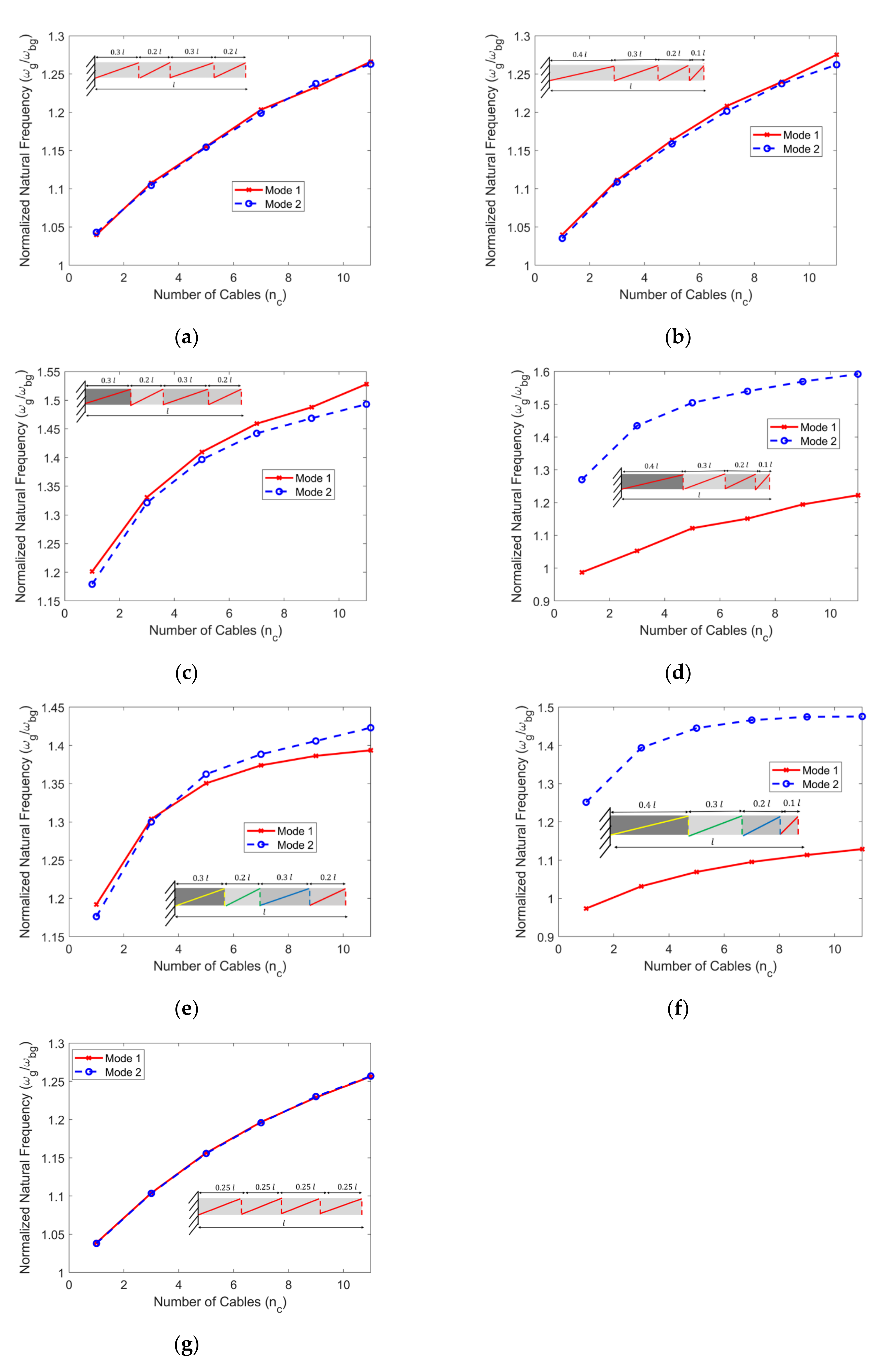
In Section 3.1, the effect of varying on the first two OP modes is studied. The wrapping patterns of different systems considered in the theoretical study are shown in Figure 2. Each element has a diagonal cable section represented by a solid line and a lumped-mass section represented by a dotted line in Figure 2. The host structures considered in Figure 2a,b are homogenous. The beam and cable sections in each fundamental element have the same material properties. In Figure 2a, the wrapping pattern has the largest element closest to the clamp end of the cantilever. In Figure 2b, each element has a different cable wrapping angle.
The system parameters selected for the analysis of homogenous structures in Figure 2a,b are shown in column 2 of Table 1. In Figure 2c–f, the same wrapping patterns as Figure 2a,b are selected. In Figure 2c,d, the beam section in each fundamental element has different material properties. The cable has the same material properties in each fundamental element. The system parameters for Figure 2c,d are shown in column 3 of Table 1. In Figure 2e,f, the beam section in each element has different material properties. The cable section in each element is also assumed to have different material properties. The system parameters for Figure 2e,f are shown in column 4 of Table 1.
In Figure 3, the number of cables is varied on the x-axis. The effective cross-section area of the cables increases with the increase in the number of cables. The coupling coefficients also become stronger with an increase in the effective area of the cables. The ratio of the natural frequencies of the CH beam (subscript denotes the mode) to the bare beam () is plotted on the y-axis of Figure 3 () for the first two OP modes. Initially, the frequencies of the respective bare beams (beams with no cable attachment) are determined.
For the homogenous host structure in Figure 3a,b, as increases, the frequencies of both the modes increase. A significant stiffening effect is observed for both modes. In Figure 3g, for the homogenous host structure with a periodic pattern (the same material and geometric parameters as column 2 of Table 1, along with the same wrapping angles), there is a significant stiffening effect like in the semi-periodic pattern case of Figure 3a. The developed generalized analytical model becomes more important when the CH structure has a non-periodic pattern. In more realistic cases of CH structures, the cables are attached in a non-periodic pattern where the material properties of the host structure and cable are different in different fundamental elements. Such cases are analyzed in Figure 3d–f. For the non-homogenous beam in Figure 3c, the frequencies of the two modes increase with . In Figure 3d, both modes show a stiffening effect. In addition, due to the vicinity of the node of the second mode to the lumped-mass section, a greater stiffening effect is observed for the second mode. Additionally, the node occurs near the element where the beam section has the lowest modulus and density. The mass effects for this case are lower, especially for the second mode.
System 1—homogenous host structure and homogenous cables; System 2—non-homogenous host structure and homogenous cables; System 3—with non-homogenous host structure and non-homogenous cables.
The case with a non-homogenous host structure and different cable properties across each element is shown in Figure 3e,f. Like the previous cases, we observe a stiffening effect in the case of the semi-periodic wrapping pattern. Additionally, with the increase in , the mass effects start to dominate for both the modes. The cable densities selected are higher for Figure 3e,f when compared to the cases of Figure 3a–d. In Figure 3f, like Figure 3d, we observe different levels of stiffening for both modes due to the node of the second mode being closer to the lumped-mass section. Due to the larger cable densities, mass effect is observed when only one cable is used, as the normalized frequency is less than one. The natural frequencies appear to approach a saturation value with the increase in the number of cables, after which it is expected to decrease due to the increase in mass effects.
This case study suggests that it is important to have a model that can consider the coupling effects in non-periodic pattern CH structures. The different natural frequency trends in Figure 3b–f, for non-periodic pattern cases, suggest different levels of mass, stiffness and coupling effects across the first two modes. The model developed in this article can be highly useful to predict the natural frequencies of CH beams where different fundamental elements have different material properties and variable wrapping angles. The coupling effects become very significant depending on the material parameters, the number of cables and the type of wrapping pattern. Hence, the development of a coupled model is highly essential for the systems with a non-periodic pattern.
3.2. Experimental Setup
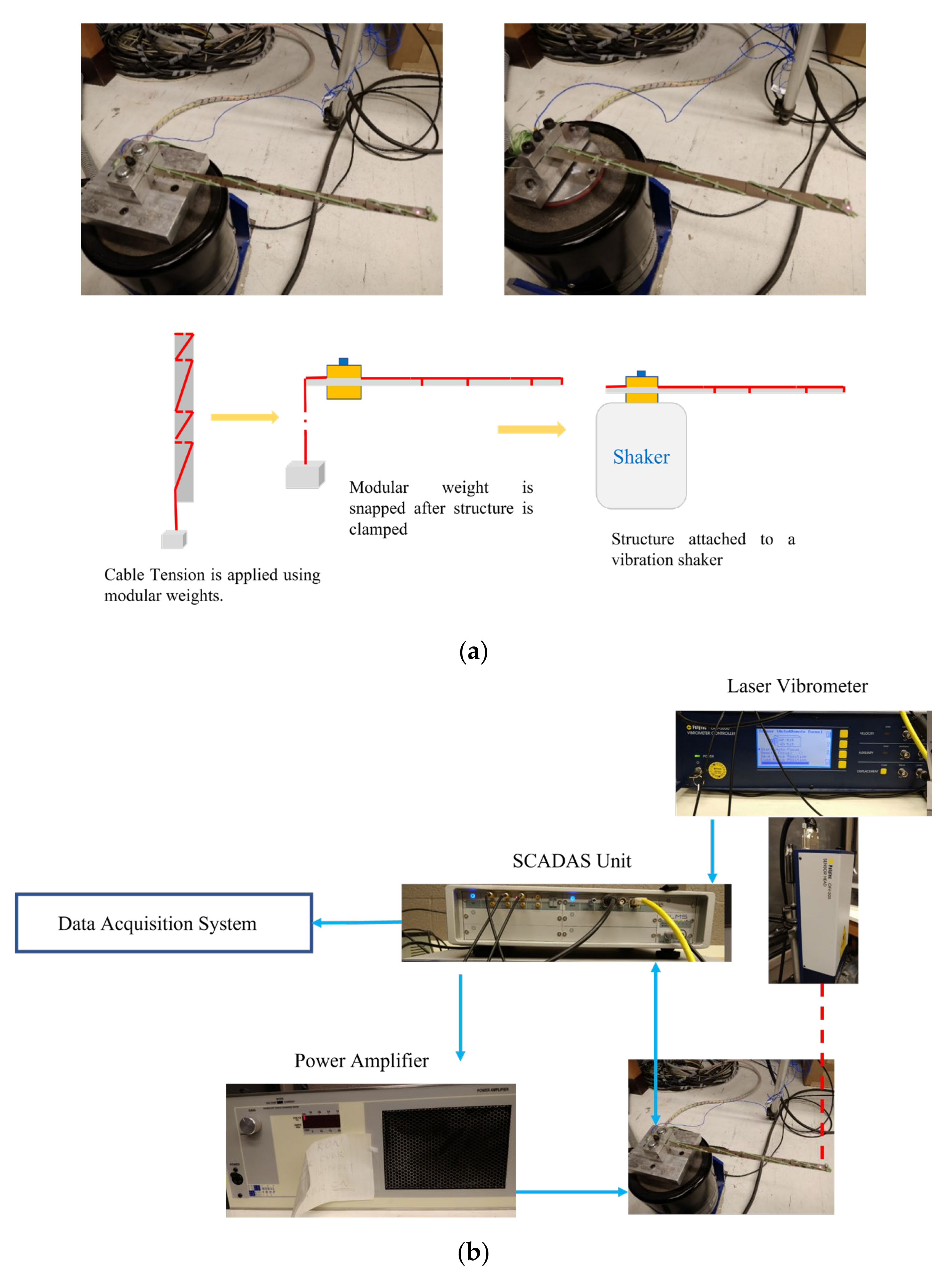
In Section 3.2, experimental investigations of two samples—wrapping pattern 1 and wrapping pattern 2—were performed. The experimental setup of the structures is shown in Figure 4a. The non-periodic pattern is described earlier in Figure 2a,b, respectively. Wrapping patterns 1 and 2 will be referred to as samples 1 and 2, respectively. The system parameters of the two samples (wrapping patterns 1 and 2) are shown in Table 2. The cable material parameters were the same as in our previous experimental characterization studies [10,12].
First, very small notches were made on the host structure and pre-tensioned cables were wrapped in a non-periodic pattern. The cable pre-tension was applied with the help of modular weights, as shown in Figure 4a. After the wrapping process, the host structure was clamped at one end to a metal fixture and the modular weights were removed. The cantilevered structure was attached to a The Modal Shop 2075E electrodynamic shaker with the help of a metal fixture. The boundary condition considered for both of the samples was that of a cantilever. Once the wrapping was complete, the beam was fixed at one end and glue was applied at discrete cable locations. Cables attached at discrete locations to the beam constituted a more realistic setup of a CH beam (see previous research by the U.S. AFRL group [1,3]). The beams were made from Al 6061 alloy metal sheets. The cable considered was a Power Pro fishing line with a strength of 80 lb [12,14]. A Siemens LMS SCM 05 SCADAS was used to define the input profile to the shaker and process the measured experimental data. The shaker motion was controlled with The Modal Shop power amplifier 2050E09. The control accelerometer used was a PCB piezotronics 352A24. The schematic of the vibration experiment, along with the instruments, is shown in Figure 4b.
The non-contact displacement sensor used was a Polytec OFV-5000 laser vibrometer, which works on the principle of the Doppler effect. Harmonic base excitation was applied to the CH beams in the OP direction. The experiment settings were defined in the Siemens LMS Sine Control Module Software. The Sine Control Module also recorded and processed the data from the experiment. To identify the torsion and IP modes, experiment mode shapes were obtained. For the torsion-dominant mode, the structure was divided into three columns. One column was along the centerline, and the other two columns were along the two edges. The sensing location resolution was 1 cm along the length. Using the data captured along multiple sensing locations, the deflection shape of the structure was obtained by the Siemens LMS software at the torsional-dominant frequency. Similarly, to find the IP frequencies, the CH beam was excited using a PCB 086C01 impact hammer.
3.3. FRF Comparison between Theory and Experiment
In Figure 5, the FRF comparison between the coupled and decoupled models with respect to the experiment FRFs are presented. The coupled model assumes the CH beam is more flexible than the decoupled model. Therefore, the FRFs of coupled theory developed in this paper match better with the experiment than those of the decoupled theory model [14], demonstrating the importance of coupling in CH beams with a non-periodic pattern. In addition, some contribution to the improvement of the frequencies from the coupled theory results from the lumped mass enhancing the already-present coupling effects that occur due to the diagonal cable, and this coupling occurs to a greater extent at peak-curvature locations.
Further discussion on curvature analysis is presented in Section 3.4. In real-world systems with significant cabling, it is important to move towards the coupled model. Additionally, the cable attachments and wrapping are rarely periodic. Hence, developing a coupled vibration model for a non-periodic CH beam with different displacements for different beam-cable fundamental elements is highly useful.
The frequencies of the model and experiment are tabulated in Table 3 and Table 4 for samples 1 and 2, respectively. The decoupled model assumptions by Martin and Salehian [14] give larger errors with respect to the experiment than the coupled model. Overall, the OP- and torsion-dominant modes show good agreement with the experiment. In addition, for the first mode of sample 2, the error of the model is larger than the higher OP modes. At the first mode, there is a possibility that the assumption that the cable remains attached everywhere on the structure contributes to model inaccuracy. The IP modes show a larger error in Table 3 and Table 4 for both the samples, as the clamping force for the cantilevered structure is predominantly in the thickness direction. In the IP direction, the clamp is not perfectly rigid, so, the error is on the higher side for the IP modes. Overall, the FRF obtained from the coupled model shows a good match with respect to the experiment.
3.4. Curvature Analysis and Mismatched Modes
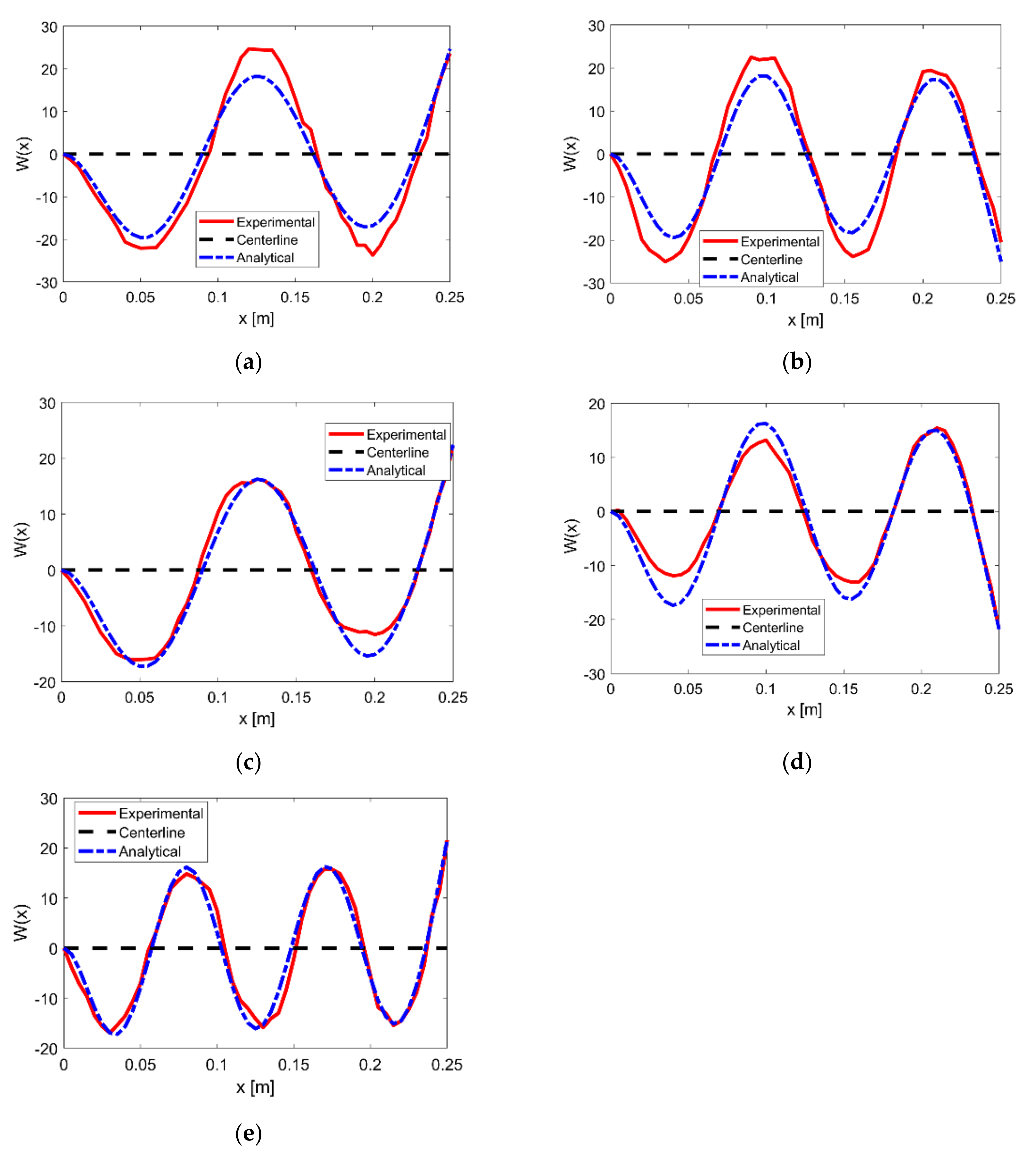
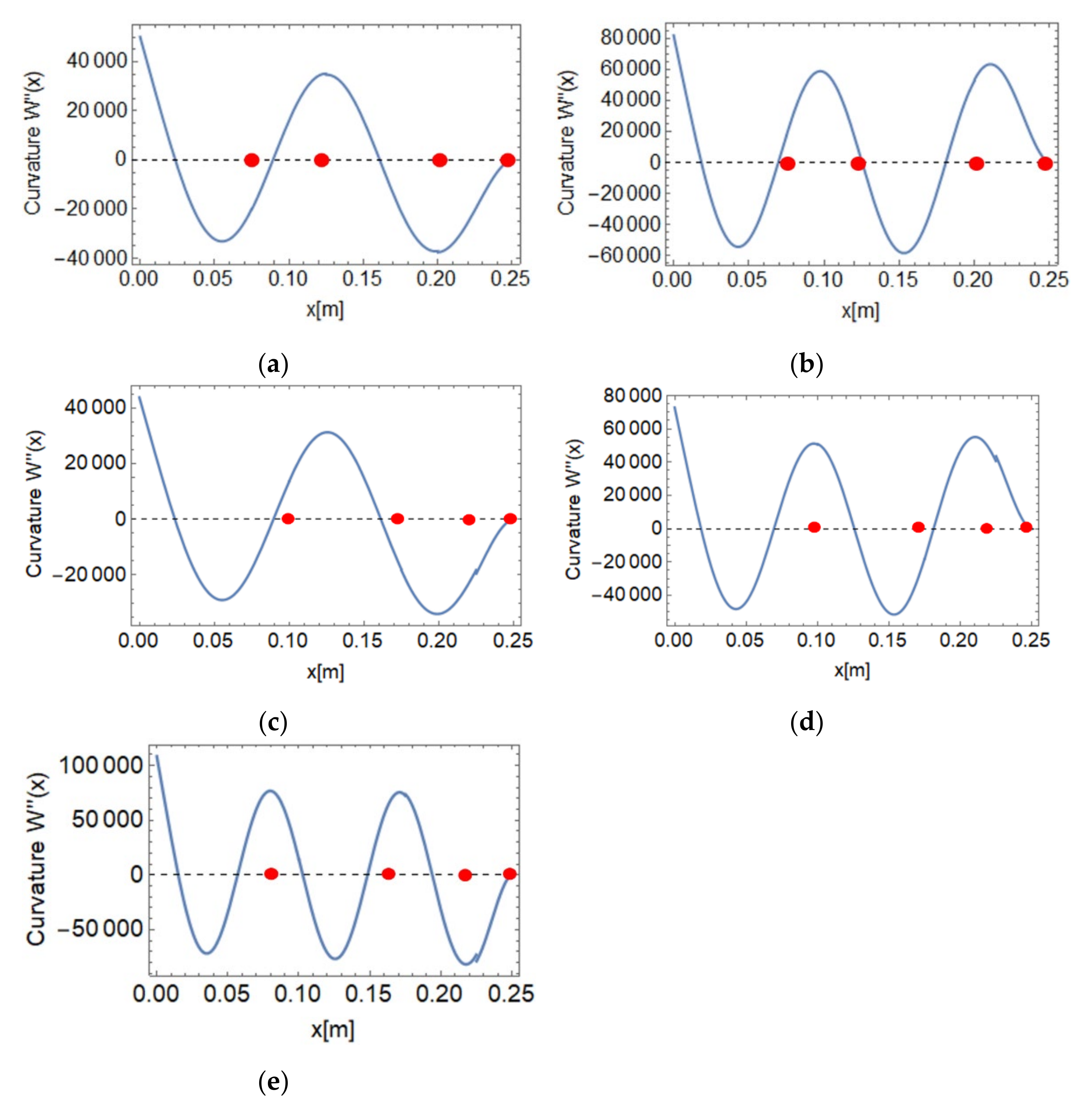
In Figure 5a, the coupled theory over-estimates the fifth mode frequency (fourth OP mode) for sample 1. The theory and experiment mode shapes are compared for modes 5 and 7 (fifth OP mode) in Figure 6a,b. To obtain the experiment mode shapes in the OP direction, the sensing is performed along the centerline with a location resolution of 0.5 cm. The node locations of OP modes 4 and 5 of the theory and experiment match well. Additionally, for sample 2 from Figure 5b, the theory under-predicts the sixth mode (fourth OP mode) and over-predicts the eighth mode (sixth OP mode). For sample 2, the mode shapes of the fourth, fifth and sixth OP modes from the theory match well with the experiment in Figure 6c–e. To obtain more insight into the mismatched modes for sample 1, the theoretical curvature is plotted for OP mode 4 (mismatched mode in FRF) and mode 5 (well-matched mode in FRF) in Figure 7a,b. The lumped-mass sections are represented by red dots in Figure 7 at the interface of the two elements. From Figure 7a, for the fourth OP mode, the second and the third peaks of the curvature are near the lumped-mass locations.
The first lumped-mass location is in the vicinity of the first curvature node. The bending stiffness of the structure is proportional to the curvature. For the mode represented in Figure 7a, the mass effect is higher as the two curvature peaks are closer to the lumped-mass locations.
Therefore, the frequency of this mode from the experiment is lower than the model frequency. In addition, some of the over-prediction from the model could also be due to the averaging approach to convert the variable coefficients into constant coefficients in Equations (9) and (10). In Figure 5b, for the fifth OP mode, the match between the theory and the experiment is good. At this mode, the three lumped-mass locations are away from the curvature peaks, so the significant mass effect observed in the fourth OP mode is not seen in the fifth OP mode.
For sample 2, the curvature plots are presented in Figure 7c–e. In Figure 7c, for the fourth OP mode, the lumped masses of the structure are near the curvature nodes. We expect larger stiffening for this mode experimentally. For the sixth OP mode, the shear effect of the cable will start to increase, which the model ignores. Because of the shear effect, the coupled model slightly over-predicts the sixth OP mode.
In addition, in sample 1, for the fourth OP mode, the peak locations of the curvature are closer to the lumped-mass locations. The presence of lumped masses near the curvature peaks enhances the coupling effect in the system. At higher modes, the number of curvature peaks increases, and the likelihood of curvature peak or node locations coinciding with the lumped-mass locations increases. This makes the coupled model highly important for the non-periodic cable-harnessed structures to accurately predict the frequencies than the decoupled model.
3.5. In-Plane-Bending- and Torsion-Dominant Experimental Mode Shapes
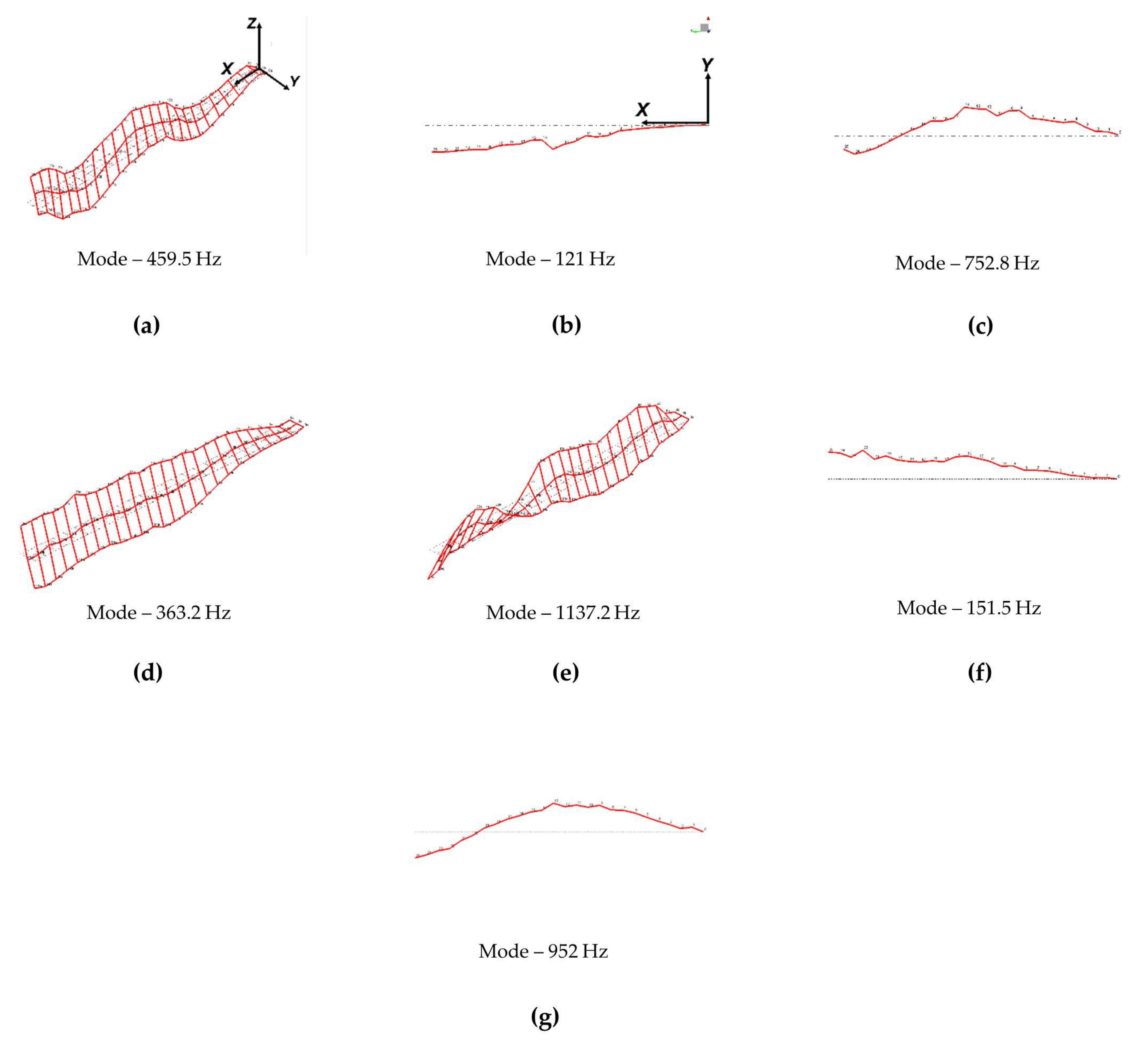
The experimental mode shapes for sample 1 of torsion- and IP-dominant modes are plotted in Figure 8a–c. As mentioned earlier in Section 3.2, to obtain these experiment mode shapes, the geometry of the experimental structures is first defined in the Siemens LMS Sine Control Module software. To obtain the torsion-dominant mode, the structure mesh is first divided into three columns (one centerline and two along the edges). Then, the geometry is meshed along the length for every 1 cm. For the several sensing locations, the motion of the structure is recorded for the torsion-dominant mode and the mode shapes obtained from the software. Similarly, to obtain the IP mode shapes, the geometry is defined along the line with 1 cm discretization in the software. The motion of the structure is obtained for several sensing locations in IP direction, and the software gives the IP mode shapes.
In the torsional-dominant mode (Figure 8a), two extreme points along the width have out-of-phase displacement. This can be observed near the free end of the beam. An IP-dominant mode has bending deformations in the X-Y plane (coordinates defined in Figure 8b). The corresponding theoretical mode shapes of sample 1 are shown in Appendix A Figure A1 to confirm their identities. In our previous work, [13], we explain the procedure to decide the mode shape dominance in a coupled system. We also observe sharp or small peaks associated with the IP mode in the experimental FRF of Figure 5a. Further, to accurately identify the IP mode, an impact test is performed. In Figure A3a, the FRF for the impact test is presented to obtain the IP frequencies. Similarly, the torsional- and IP-dominant experimental mode shapes for sample 2 are presented in Figure 8d–g, and the FRF from the impact test is presented in Figure A3b for the IP frequencies. The corresponding mode shapes from the theory for the torsion and IP modes are presented in Figure A2 for sample 2.
4. Conclusions
In this article, a fully coupled vibration model is developed to analyze CH beams with a non-periodic wrapping pattern. For the theoretical studies, both homogenous and non-homogenous structures were selected. In the theoretical studies, the number of cables was varied and their effect on the normalized coupled natural frequencies of both homogenous and non-homogenous structures was studied. It was observed that homogenous structures show a significant stiffening effect for the first two OP-dominant modes. In the non-homogenous host structure and the homogenous cable system, the stiffening effect is higher for a lower number of cables and the mass effects start to dominate as the number of cables increases. In non-homogenous host structures and non-homogenous cable systems, the natural frequencies tend to approach a saturation value due to the mass effect of the high-density cables in some of the fundamental element sections. In addition, for the wrapping pattern with the smallest element near the tip of the cantilever, the second mode shows a significantly greater stiffening effect than the first mode. This is due to the proximity of the node of the second mode to the lumped-mass cable section. The node occurs near the beam section, which has the lowest modulus and density. The theoretical study showed how variation in material properties and wrapping angles across different fundamental elements changes the natural frequencies.
Two samples with homogenous beam structures and homogenous cables were experimentally investigated. The FRF from the coupled model matched better with the experiment FRF than the decoupled FRF. The SE in the OP-dominant mode depended on the curvature. Employing the coupled model of this paper provided improvement in predicting the natural frequencies, especially for higher modes where the peak or node locations of the curvature were in the vicinity of lumped-mass locations. In real-world space structures, the amount of cable harnessing on the host structure is significant; they are mostly non-periodic and the host structures are non-homogenous. For such systems, it is advantageous to move towards a model that takes into consideration the material non-homogeneity, variable wrapping angles, and the coupling effects, to accurately predict the mass and stiffening effects due to cable harnessing.
Author Contributions
K.Y.—Conceptualization, mathematical modeling, numerical simulation, experimental investigations, analysis, manuscript writing; B.M.—Mathematical modeling and manuscript writing; P.A.—Literature review, discussion and manuscript writing; A.S.—Funding acquisition, project guidance, manuscript writing. All authors have read and agreed to the published version of the manuscript.
Funding
This research received no external funding.
Data Availability Statement
The data used to support the findings of this study can be made available upon request to the authors.
Acknowledgments
The authors thank the Natural Sciences and Engineering Research Council of Canada funding agency in Canada, grant number NSERC-DG 371472-2009 for supporting this research through Salehian’s Discovery Grant Program. The APC charges are waived by the publisher in this invited article. The authors would also like to thank Kirsten Morris for engaging in insightful discussions.
Conflicts of Interest
The authors declare no conflict of interest in preparing this article.
Nomenclature
| Cross-sectional area of the beam and the cable | |
| Width of the beam | |
| Thickness of the beam | |
| Strain energy coefficients for Euler–Bernoulli based model of ith fundamental element | |
| Strain energy coefficients for the constant coefficient model of ith fundamental element | |
| Kinetic energy coefficients of ith fundamental element | |
| Kinetic energy coefficients of the constant coefficient model of ith fundamental element | |
| Length of the beam | |
| Number of cables | |
| Radius of the cable | |
| Pre-tension of the cables | |
| Base excitation | |
| , | Actuation and sensing location |
| , | y and z coordinates of the cable where strains are evaluated |
| Wrapping angle of ith element | |
| Excitation frequency | |
| Natural frequency of the mode for cable-harnessed beam | |
| Natural frequency of the mode for beam with no cable | |
| Length of ith fundamental element | |
| Beam and cable densities of ith fundamental element | |
| Beam and cable Young’s modulus of ith fundamental element | |
| Beam and cable shear modulus of ith fundamental element | |
| Lumped-mass effect due to the horizontal part of the cable in the axial, in-plane bending, out-of-plane bending and torsional directions of ith fundamental element | |
| Displacement components at all points of the body of the beam | |
| Velocity components at all points of the body of the beam |
Appendix A
The intermediate derivation steps to obtain Equations (9) and (10) are shown below in Equation (A1). The higher-order terms (order ) are neglected in the strain energy.
The coefficients for the averaged strain energy and kinetic energy expressions, Equations (12) and (13), are as follows:
The strain and kinetic energy expressions for the entire system are shown in Equations (A4) and (A5):
The expressions for in Equations (18) and (A7) are shown below:
The continuity conditions are shown in Equation (A7):
Regarding the continuity conditions in Equation (A7), the displacement in first and eleventh rows; and the slope in second and twelfth rows; of the axial and torsion motion are assumed to be continuous. In rows three to six, IP and rows seven to ten OP; displacement; slope; moment; and shear are assumed to be continuous.
The mode shape parameter can be written in terms of . The spatial solutions , and are shown in Equation (A8):
where represents the elements of matrix []. To satisfy the condition in Equation (A8), the spatial solutions should be as in Equation (A9):
To mimic the conditions that will be used for experimental testing, the effect of base excitation at the clamped end must be introduced in the fully coupled equations of motion. The base excitation assumed is harmonic and is of the form , where is the base acceleration and is the forcing frequency. The equations after including the effect of base excitation can be formulated similarly to in [10,28,29], and are shown in Equation (A10):
where is the relative displacement in the OP direction with respect to the base. The procedure to obtain FRF is outlined in Equations (A11)–(A14). The readers may refer to the previous works by our group [10,14] regarding the detailed steps for incorporating the effect of base excitation to arrive at the final frequency response function. The solution for the steady-state relative displacement is as follows:
where is the natural frequency. The total displacement of the structure, after including , is shown in Equation (A13):
The expression for the FRF is as in Equation (A14):
The theoretical mode shapes of sample 1 and sample 2 that are referred to in Section 3.5 are shown in this Appendix A. The mode shapes for sample 1 are shown in Figure A1 and for sample 2 in Figure A2. The experimental IP bending FRFs are shown in Figure A3 for both samples.
Figure A1.
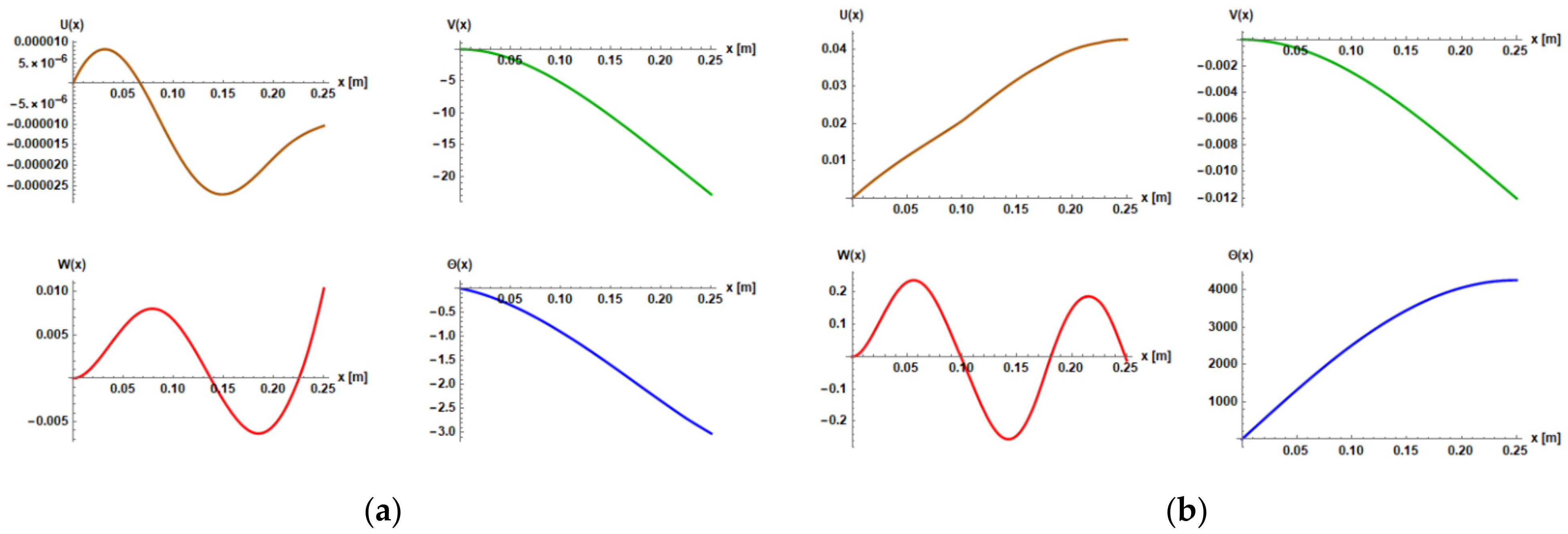
Coupled theoretical mode shapes for sample 1: (a) first IP mode; (b) first torsion mode; (c) second IP mode.
Figure A1.
Coupled theoretical mode shapes for sample 1: (a) first IP mode; (b) first torsion mode; (c) second IP mode.

Figure A2.
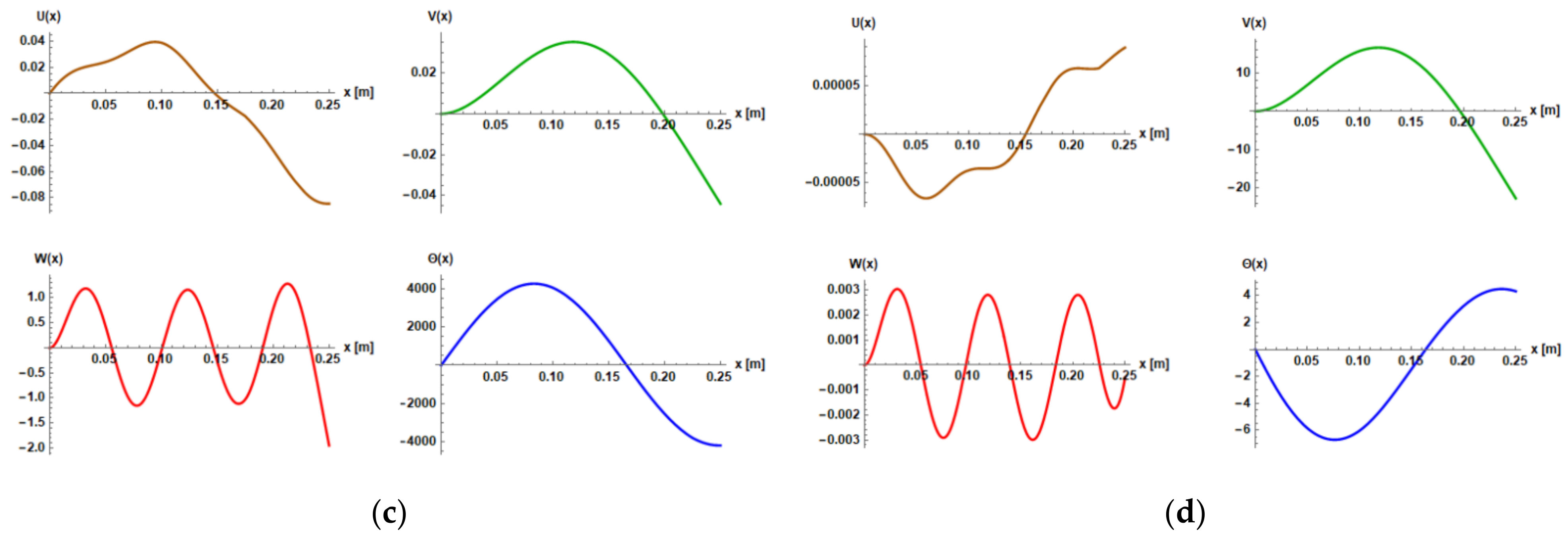
Coupled theoretical mode shapes for sample 2: (a) first IP mode; (b) first torsion mode; (c) second torsion mode; (d) second IP mode.
Figure A2.
Coupled theoretical mode shapes for sample 2: (a) first IP mode; (b) first torsion mode; (c) second torsion mode; (d) second IP mode.


Figure A3.
IP FRF obtained from impact testing for: (a) sample 1; (b) sample 2.

References
- Babuska, V.; Coombs, D.M.; Goodding, J.C.; Ardelean, E.V.; Robertson, L.M.; Lane, S.A. Modeling and experimental validation of space structures with wiring harnesses. J. Spacecr. Rockets 2010, 47, 1038–1052. [Google Scholar] [CrossRef]
- Robertson, L.; Lane, S.; Ingram, B.; Hansen, E.; Babuska, V.; Goodding, J.; Mimovich, M.; Mehle, G.; Coombs, D.; Ardelean, E. Cable effects on the dynamics of large precision structures. In Proceedings of the 48th AIAA/ASME/ASCE/AHS/ASC Structures, Structural Dynamics, and Materials Conference, Honolulu, HI, USA, 23–26 April 2007; p. 2389. [Google Scholar]
- Goodding, J.C.; Ardelean, E.V.; Babuska, V.; Robertson, L.M., III; Lane, S.A. Experimental techniques and structural parameter estimation studies of spacecraft cables. J. Spacecr. Rockets 2011, 48, 942–957. [Google Scholar] [CrossRef]
- Coombs, D.M.; Goodding, J.C.; Babuška, V.; Ardelean, E.V.; Robertson, L.M.; Lane, S.A. Dynamic modeling and experimental validation of a cable-loaded panel. J. Spacecr. Rockets 2011, 48, 958–974. [Google Scholar] [CrossRef]
- Kauffman, J.L.; Lesieutre, G.A.; Babuška, V. Damping models for shear beams with applications to spacecraft wiring harnesses. J. Spacecr. Rockets 2014, 51, 16–22. [Google Scholar] [CrossRef]
- Kauffman, J.L.; Lesieutre, G.A. Damping models for timoshenko beams with applications to spacecraft wiring harnesses. In Proceedings of the 54th AIAA/ASME/ASCE/AHS/ASC Structures, Structural Dynamics, and Materials Conference, Boston, MA, USA, 8–11 April 2013; p. 1890. [Google Scholar]
- Spak, K. Modeling Cable Harness Effects on Space Structures. Ph.D. Thesis, Virginia Tech, Blacksburg, VA, USA, 2014. [Google Scholar]
- Spak, K.S.; Agnes, G.S.; Inman, D.J. Bakeout effects on dynamic response of spaceflight cables. J. Spacecr. Rockets 2014, 51, 1721–1734. [Google Scholar] [CrossRef]
- Martin, B.; Salehian, A. Mass and stiffness effects of harnessing cables on structural dynamics: Continuum modeling. AIAA J. 2016, 54, 2881–2904. [Google Scholar] [CrossRef]
- Martin, B.; Salehian, A. Homogenization modeling of periodically wrapped string-harnessed beam structures: Experimental validation. AIAA J. 2016, 54, 3965–3980. [Google Scholar] [CrossRef]
- Agrawal, P.; Salehian, A. Damping Mechanisms in Cable-Harnessed Structures for Space Applications: Analytical Modeling. J. Vib. Acoust. 2020, 143, 021001. [Google Scholar] [CrossRef]
- Yerrapragada, K.; Salehian, A. Coupled dynamics of cable-harnessed structures: Experimental validation. J. Vib. Acoust. Trans. ASME 2019, 141, 061001. [Google Scholar] [CrossRef] [Green Version]
- Yerrapragada, K.; Salehian, A. Analytical Study of Coupling Effects for Vibrations of Cable-Harnessed Beam Structures. J. Vib. Acoust. 2019, 141, 031001. [Google Scholar] [CrossRef] [Green Version]
- Martin, B.; Salehian, A. Continuum Modeling of Nonperiodic String-Harnessed Structures: Perturbation Theory and Experiments. AIAA J. 2019, 57, 1736–1751. [Google Scholar] [CrossRef]
- Banerjee, J.R. Frequency equation and mode shape formulae for composite Timoshenko beams. Compos. Struct. 2001, 51, 381–388. [Google Scholar] [CrossRef]
- Amoozgar, M.; Bodaghi, M.; Ajaj, M.R. The effect of non-conservative compressive force on the vibration of rotating composite blades. Vibration 2020, 3, 478–490. [Google Scholar] [CrossRef]
- Wang, Q.; Wang, Z.; Fan, B. Coupled bending and torsional vibration characteristics analysis of inhomogeneous wind turbine tower with variable cross section under elastic constraint. Appl. Math. Model. 2021, 93, 188–205. [Google Scholar] [CrossRef]
- Mei, C. Effect of material coupling on wave vibration of composite Timoshenko beams. J. Vib. Acoust. Trans. ASME 2005, 127, 333–340. [Google Scholar] [CrossRef]
- Yerrapragada, K.; Salehian, A. Multi-Dimensional Vibrations of Cable-Harnessed Beam Structures with Periodic Pattern: Modeling and Experiment. Shock. Vib. 2022, 2022, 7343582. [Google Scholar]
- Yerrapragada, K. Coupled Dynamics of Cable-Harnessed Structures: Analytical Modeling and Experimental Validation. Ph.D. Thesis, University of Waterloo, Waterloo, ON, Canada, 2019. [Google Scholar]
- Stoykov, S.; Ribeiro, P. Vibration analysis of rotating 3D beams by the p-version finite element method. Finite Elem. Anal. Des. 2013, 65, 76–88. [Google Scholar] [CrossRef]
- Stoykov, S.; Ribeiro, P. Nonlinear forced vibrations and static deformations of 3D beams with rectangular cross section: The influence of warping, shear deformation and longitudinal displacements. Int. J. Mech. Sci. 2010, 52, 1505–1521. [Google Scholar] [CrossRef]
- Rao, S.S. Vibration of Continuous Systems; John Wiley & Sons: Hoboken, NJ, USA, 2019. [Google Scholar]
- Hagedorn, P.; DasGupta, A. Vibrations and Waves in Continuous Mechanical Systems; John Wiley & Sons: West Sussex, UK, 2007. [Google Scholar]
- Karami, M.A.; Inman, D.J. Analytical modeling and experimental verification of the vibrations of the zigzag microstructure for energy harvesting. J. Vib. Acoust. 2011, 133, 11002. [Google Scholar] [CrossRef]
- Ansari, M.H.; Karami, M.A. Energy harvesting from heartbeat using piezoelectric beams with fan-folded configuration and added tip mass. In ASME Smart Materials, Adaptive Structures and Intelligent Systems Conference; ASME: Colorado Springs, CO, USA, 2015; Volume 57304, p. V002T07A020. [Google Scholar]
- Ansari, M.H.; Karami, M.A. Modeling and experimental verification of a fan-folded vibration energy harvester for leadless pacemakers. J. Appl. Phys. 2016, 119, 94506. [Google Scholar] [CrossRef]
- Erturk, A.; Inman, D.J. An experimentally validated bimorph cantilever model for piezoelectric energy harvesting from base excitations. Smart Mater. Struct. 2009, 18, 25009. [Google Scholar] [CrossRef]
- Erturk, A.; Inman, D.J. Piezoelectric Energy Harvesting; John Wiley & Sons: West Sussex, UK, 2011. [Google Scholar]
Figure 1.
(a) Representation of homogenous non-periodically wrapped CH beam; (b) local element with its coordinate system.
Figure 1.
(a) Representation of homogenous non-periodically wrapped CH beam; (b) local element with its coordinate system.

Figure 2.
Top view representation of CH beams with non-periodic wrapping pattern: (a,b) homogenous host structure and homogenous cables; (c,d) non-homogenous host structure and homogenous cables; (e,f) non-homogenous host structure and non-homogenous cable attachments.
Figure 2.
Top view representation of CH beams with non-periodic wrapping pattern: (a,b) homogenous host structure and homogenous cables; (c,d) non-homogenous host structure and homogenous cables; (e,f) non-homogenous host structure and non-homogenous cable attachments.

Figure 3.
Effect of number of wrapped cables on the normalized natural frequency of first two modes for: (a,b) homogenous beam and cables; (c,d) non-homogenous beam and homogenous cables; (e,f) non-homogenous beam and non-homogenous cables. (g) Periodic wrapping pattern.
Figure 3.
Effect of number of wrapped cables on the normalized natural frequency of first two modes for: (a,b) homogenous beam and cables; (c,d) non-homogenous beam and homogenous cables; (e,f) non-homogenous beam and non-homogenous cables. (g) Periodic wrapping pattern.

Figure 4.
(a) Vibration experiment setup of the samples of CH beams with non-periodic wrapping pattern on the shaker, along with the schematic of the structure attachment to the shaker; (b) schematic of the vibration experiment on the CH beam, along with the instruments used.
Figure 4.
(a) Vibration experiment setup of the samples of CH beams with non-periodic wrapping pattern on the shaker, along with the schematic of the structure attachment to the shaker; (b) schematic of the vibration experiment on the CH beam, along with the instruments used.

Figure 5.
Coupled and decoupled analytical FRFs and experiment FRF for: (a) sample 1; (b) sample 2.

Figure 6.
Experimental and theory OP mode shapes for sample 1—(a) mode 5, and (b) mode 7; for sample 2—(c) mode 6, (d) mode 7, and (e) mode 8.
Figure 6.
Experimental and theory OP mode shapes for sample 1—(a) mode 5, and (b) mode 7; for sample 2—(c) mode 6, (d) mode 7, and (e) mode 8.

Figure 7.
Theoretical plots for curvature for sample 1—(a) mode 5, and (b) mode 7; for sample 2—(c) mode 6, (d) mode 7, and (e) mode 8. ![Vibration 05 00015 i001]() represents position of lumped-mass section.
represents position of lumped-mass section.
 represents position of lumped-mass section.
Figure 7.
Theoretical plots for curvature for sample 1—(a) mode 5, and (b) mode 7; for sample 2—(c) mode 6, (d) mode 7, and (e) mode 8. ![Vibration 05 00015 i001]() represents position of lumped-mass section.
represents position of lumped-mass section.
represents position of lumped-mass section.
Figure 8.
Experiment mode shape: sample 1—(a) first torsion mode at 459.5 Hz, (b) first IP mode at 121 Hz, and (c) second IP mode at 752.8 Hz; for sample 2—(d) first torsion mode at 363.2 Hz, (e) second torsion mode at 1137.2 Hz, (f) first IP mode at 151.5 Hz, and (g) second IP mode at 952 Hz.
Figure 8.
Experiment mode shape: sample 1—(a) first torsion mode at 459.5 Hz, (b) first IP mode at 121 Hz, and (c) second IP mode at 752.8 Hz; for sample 2—(d) first torsion mode at 363.2 Hz, (e) second torsion mode at 1137.2 Hz, (f) first IP mode at 151.5 Hz, and (g) second IP mode at 952 Hz.


Table 1.
System parameters used in theoretical studies with combinations of homogenous and non-homogenous host structure and cable non-periodic wrapping pattern.
Table 1.
System parameters used in theoretical studies with combinations of homogenous and non-homogenous host structure and cable non-periodic wrapping pattern.
| Parameters | System 1 | System 2 | System 3 |
|---|---|---|---|
| Beam length () [mm] | 250 | 250 | 250 |
| Beam width () [mm] | 10 | 10 | 10 |
| Beam thickness () [mm] | 0.782 | 0.782 | 0.782 |
| No. of fundamental elements | 4 | 4 | 4 |
| Cable radius () [mm] | 0.21 | 0.21 | 0.21 |
| Pre-tension of cables () [N] | 4 | 4 | 4 |
| Density of each beam element [kg/m3] | |||
| 2768 | 2768 | 2768 | |
| 2768 | 7850 | 7850 | |
| 2768 | 1100 | 1100 | |
| 2768 | 8790 | 8790 | |
| Young’s Modulus of each beam element [GPa] | |||
| 68.9 | 68.9 | 68.9 | |
| 68.9 | 210 | 210 | |
| 68.9 | 5 | 5 | |
| 68.9 | 121 | 121 | |
| Shear Modulus of each beam element [GPa] | |||
| 25.7 | 25.7 | 25.7 | |
| 25.7 | 81 | 81 | |
| 25.7 | 1.8 | 1.8 | |
| 25.7 | 43.2 | 43.2 | |
| Density of each cable element [kg/m3] | |||
| 1400 | 1400 | 1400 | |
| 1400 | 1400 | 7850 | |
| 1400 | 1400 | 1400 | |
| 1400 | 1400 | 8790 | |
| Young’s Modulus of each cable element [GPa] | |||
| 128.04 | 128.04 | 128.04 | |
| 128.04 | 128.04 | 210 | |
| 128.04 | 128.04 | 128.04 | |
| 128.04 | 128.04 | 121 |
Table 2.
Parameters of two CH beams in experiment investigations.
| System Parameters | Sample 1 | Sample 2 |
|---|---|---|
| Width () [mm] | 10 | 13.1 |
| Thickness () [mm] | 0.782 | 0.782 |
| Length () [mm] | 250 | 250 |
| Number of Cables | 9 | 8 |
| Cable pre-tension () [N] | 14 | 14 |
| Number of fundamental elements () | 4 | 4 |
| Beam density () [kg/m3] | 2768 | 2768 |
| Beam modulus of elasticity () [GPa] | 68.9 | 68.9 |
| Cable radius () [mm] | 0.21 | 0.21 |
| Beam shear modulus () [GPa] | 25.7 | 25.7 |
| Cable density () [kg/m3] | 1400 | 1400 |
| Cable modulus of elasticity () [GPa] | 128.04 | 128.04 |
Table 3.
Coupled, decoupled and experiment natural frequencies of sample 1.
| Mode No | Experiment [Hz] | Coupled [Hz] | Decoupled [Hz] | % Coupled and Experiment | % Decoupled and Experiment |
|---|---|---|---|---|---|
| 1 | 13.2 (OP) | 12.5 | 16.6 | −5.5% | 26.1% |
| 2 | 78.6 (OP) | 78.2 | 104.2 | −0.5% | 32.5% |
| 3 | 121.0 (IP) | 140.3 | - | 15.9% | - |
| 4 | 215.7 (OP) | 218.9 | 291.9 | 1.5% | 35.3% |
| 5 | 384.8 (OP) | 429.8 | 570.0 | 11.7% | 48.1% |
| 6 | 459.5 (Torsion) | 447.1 | - | −2.7% | - |
| 7 | 709.1 (OP) | 706.4 | 946.3 | −0.4% | 33.4% |
| 8 | 752.8 (IP) | 879.9 | - | 16.9% | - |
Table 4.
Coupled, decoupled, and experiment natural frequencies of sample 2.
| Mode No | Experiment [Hz] | Coupled [Hz] | Decoupled [Hz] | % Coupled and Experiment | % Decoupled and Experiment |
|---|---|---|---|---|---|
| 1 | 13.7 (OP) | 11.9 | 14.9 | −13.1% | 8.9% |
| 2 | 76.9 (OP) | 74.7 | 93.3 | −2.8% | 21.3% |
| 3 | 151.5 (IP) | 179.7 | - | 18.6% | - |
| 4 | 213.4 (OP) | 208.8 | 260.7 | −2.2% | 22.1% |
| 5 | 363.2 (Torsion) | 347.0 | - | −4.5% | - |
| 6 | 438.9 (OP) | 407.4 | 511.5 | −7.2% | 16.5% |
| 7 | 679.0 (OP) | 675.2 | 843.4 | −0.6% | 24.2% |
| 8 | 965.7 (OP) | 1008.1 | 1256.0 | 4.4% | 30.1% |
| 9 | 1137.2 (Torsion) | 1045.3 | - | −8.1% | - |
| 10 | 952.0 (IP) | 1123.5 | - | 18.0% | - |
Publisher’s Note: MDPI stays neutral with regard to jurisdictional claims in published maps and institutional affiliations. |
© 2022 by the authors. Licensee MDPI, Basel, Switzerland. This article is an open access article distributed under the terms and conditions of the Creative Commons Attribution (CC BY) license (https://creativecommons.org/licenses/by/4.0/).
Share and Cite
MDPI and ACS Style
Yerrapragada, K.; Martin, B.; Agrawal, P.; Salehian, A. Fully Coupled Vibrations of Cable-Harnessed Beams with a Non-Periodic Wrapping Pattern. Vibration 2022, 5, 238-263. https://doi.org/10.3390/vibration5020015
AMA Style
Yerrapragada K, Martin B, Agrawal P, Salehian A. Fully Coupled Vibrations of Cable-Harnessed Beams with a Non-Periodic Wrapping Pattern. Vibration. 2022; 5(2):238-263. https://doi.org/10.3390/vibration5020015
Chicago/Turabian StyleYerrapragada, Karthik, Blake Martin, Pranav Agrawal, and Armaghan Salehian. 2022. "Fully Coupled Vibrations of Cable-Harnessed Beams with a Non-Periodic Wrapping Pattern" Vibration 5, no. 2: 238-263. https://doi.org/10.3390/vibration5020015