
Safety and Risk Analysis of Autonomous Vehicles Using Computer Vision and Neural Networks


1
Center of Excellence for Autonomous Vehicle Research, Department of Mechanical Engineering, Vellore Institute of Technology, Vellore 632014, Tamil Nadu, India
2
Automotive Research Center, Department of Mechanical Engineering, Vellore Institute of Technology, Vellore 632014, Tamil Nadu, India
3
Entrepreneuriat Territoire Innovation (ETI), Groupe de Recherche en Gestion des Organisations (GREGOR), IAE Paris—Sorbonne Business School, Université Paris 1 Panthéon-Sorbonne, 75013 Paris, France
4
Live + Smart Research Lab, School of Architecture and Built Environment, Deakin University, Geelong, VIC 3220, Australia
*
Author to whom correspondence should be addressed.
Vehicles 2021, 3(3), 595-617; https://doi.org/10.3390/vehicles3030036
Submission received: 9 July 2021
/
Revised: 3 September 2021
/
Accepted: 8 September 2021
/
Published: 15 September 2021
(This article belongs to the Special Issue Driver-Vehicle Automation Collaboration)
Abstract
:The autonomous vehicle (AVs) market is expanding at a rapid pace due to the advancement of information, communication, and sensor technology applications, offering a broad range of opportunities in terms of energy efficiency and addressing climate change concerns and safety. With regard to this last point, the rate of reduction in accidents is considerable when switching safety control tasks to machines from humans, which can be noted as having significantly slower response rates. This paper explores this thematic by focusing on the safety of AVs by thorough analysis of previously collected AV crash statistics and further discusses possible solutions for achieving increased autonomous vehicle safety. To achieve this, this technical paper develops a dynamic run-time safe assessment system, using the standard autonomous drive system (ADS), which is developed and simulated in case studies further in the paper. OpenCV methods for lane detection are developed and applied as robust control frameworks, which introduces the factor of vehicle crash predictability for the ego vehicle. The developed system is made to predict possible crashes by using a combination of machine learning and neural network methods, providing useful information for response mechanisms in risk scenarios. In addition, this paper explores the operational design domain (ODD) of the AV’s system and provides possible solutions to extend the domain in order to render vehicle operationality, even in safe mode. Additionally, three case studies are explored to supplement a discussion on the implementation of algorithms aimed at increasing curved lane detection ability and introducing trajectory predictability of neighbouring vehicles for an ego vehicle, resulting in lower collisions and increasing the safety of the AV overall. This paper thus explores the technical development of autonomous vehicles and is aimed at researchers and practitioners engaging in the conceptualisation, design, and implementation of safer AV systems focusing on lane detection and expanding AV safe state domains and vehicle trajectory predictability.
1. Introduction
An Autonomous Vehicle (AV) is able to perform partial or complete functions, including, i.a., driving, parking, and lane maintaining, with indirect supervision from the driver or no supervision at all. With upcoming trends, it is noted that vehicle automation, vehicle electrification, and ride sharing will aid in unleashing the potential of AVs [1]. Experts predict that these trends will revolutionize the transport industry by 2050, with vehicle safety being the primary concern of AV developers [2] At the time of writing, it is noted that there are numerous AV safety related technologies that can assist drivers, such as features including drift prevention to adjacent lanes, unsafe sudden lane changes, sudden or gradual braking (when there is an obstacle), consequent change of lane (whenever braking is not sufficient), etc. [3,4]. For the above mentioned features, AVs rely primarily on two systems, namely the autonomous drive systems (ADS) and advanced driver-assistance systems (ADAS), to manage all incoming inputs in order to respond with corresponding output functions. These systems are used to make important decisions such as course correction, lane detection, lane keeping, proactive braking, pedestrian detection etc. with the use of methods such as Hough Line transforms, Neural Networks (NNs), Co-operative Collision Avoidance (CCA) algorithms, Markov Decision Processes (MDPs), Robust Control Planning etc. [5,6,7,8]. The main sources of input to AV driving and decision making are noted to be from light detection and ranging (LIDAR), radio detection and ranging (RADAR), camera, and other related sensors [9]. Though there are many sensors and communication technologies built into AVs, there are factors of risk involved which need to be properly addressed. These risks can occur in scenarios which are highly spontaneous and dynamic where AV systems are not able to distinguish a curved from a straight road, to navigate foggy conditions, to predict movements of surrounding vehicles, to judge high speed lane changes, etc. [10]. These risks can, however, be solved by updating and operating AVs in a safe state of the operational design domain (ODD) using OpenCV, improving the detection of curved lanes and predicting a neighbouring vehicle’s trajectory using model-based reinforcement learning algorithms [11].
For example, Alphabet’s Waymo has been reported to have developed similar technologies and the abovementioned methods, where it is claimed that their AV model has completed up to 20 million miles (equivalent to 32 million KM) on a complete autonomous drive [12], which is a significant milestone to reach market use. This leads to a substantial pool of data collected by the system’s LIDAR and subsequent cameras, where the data are stored both on the car’s in-built computer and synchronized through centralized systems for processing. On this front, the stored data are divided into training and validation datasets and then learned by the ADS system which updates the ODD, thus increasing the safe state domain [13]. This also improves the accuracy and confidence of the autonomous vehicle, particularly on curved lane detection, which is a complex domain requiring research attention. They have also claimed that the AV is operable in foggy conditions where it has been reported that it covered the entire Phoenix valley of 517 square miles (equivalent to 832 sq. Kilometers) [14].
There has been much research and development in lane prediction, where vehicles may calculate possible trajectories of their neighbouring vehicles by using robust planning with continuous ambiguity [15]. The robust planning continuously predicts and correspondingly adjusts the AV’s trajectory and speed in accordance with the neighbouring vehicles. The AVs also use the spatial convolutional neural network (SCNN) method for better detection of spatial features of neighbouring objects and their dynamics. One of the major risks involved is AV and pedestrian collision, which can be addressed through the use of vehicle-to-everything (V2X) communication technology, which warns other vehicles and pedestrians in the path of an oncoming vehicle [16]. These risks and their consequences must be taken into account when designing autonomous drive systems.
Different studies are conducted in this paper to develop the safety of AVs, with their foundation being the vehicle’s ability to predict lanes, including both straight and curved lanes, and the AV’s ability to predict the behaviour of neighbouring vehicles, decreasing the probability of crashes and increasing the overall safety of the vehicle and its occupants. For the first case, detection of lanes, the paper presents an algorithm using Hough transforms, enabling the AV to detect straight lanes. In the second case, we address the shortcomings of the first study, where the algorithm used is modified so that the AV can detect and measure the curvature of curved lanes. The final study explores the predictability feature of the AV by simulating an ego vehicle in three environments: (1) the highway environment (highway-env), which involves an AV trying to manoeuvre through traffic in a four-lane road; (2) the merging of lanes environment (merge-of-lanes-env), in which the highway is merged with an adjacent lane, and the AV is tested for incoming traffic from the adjacent lane; and (3) the roundabout environment (roundabout-env), which consists of a standard roundabout with incoming vehicles. A shortcoming of the model is noted, and an improved algorithm is proposed and tested. These are further discussed in the paper.
Throughout the above, the primary aims and contributions of the paper are as follows:
- The interaction between the ADS and the operational design domain (ODD) is studied for various states, and it is analysed with regard to how a safe state ODD can be maintained.
- Various concepts and factors involved in the design of safety and risk assessment systems are explained, such as required human–machine interactions (HMIs), vehicle-to-everything V2X communication, and other factors required for AVs’ ground reality.
- Technical machine learning approaches are discussed, such as the partially observable Markov decision process (POMPD) model, the model predictive control (MPC) model, and other neural network methods such as spatial convolutional neural networks (SCNN) and convolutional neural networks (CNNs).
- A detailed study about cooperative collision avoidance (CCA) for connected vehicles is introduced.
- Case studies on the lane detection of straight lanes and modifying the straight lane detection algorithm for the detection of curved lanes are conducted.
- The neighbouring vehicle’s trajectory is predicted using robust control frameworks, thereby achieving higher predictability in an ego vehicle.
2. Concepts and Factors Involved in the Design of Safety and Risk Assessment in AVs
This section discusses concepts and factors required for designing and assessing the safety and risks in AVs.
2.1. Operational Design Domains and OREMs
An operational design domain (ODD) is a set of scenarios and situations which indirectly represents the requirements of given automation features. SAE J3016 defines an ODD as a set of operating conditions under which a given driving automation system is specifically designed to function, including environmental, geographical, and time-of-day restrictions, with or without the requisite absence or presence of certain traffic characteristics [7,17,18]. ADS and ADAS depend on these learned and pre-analysed scenarios to make important decisions related to the mode of operation of vehicles. The ODD also includes various driving scenarios including low speed assist, cruising assist, urban lane driving, mountainous and off road driving, etc. The ADS has one or more such features, and, correspondingly, each of those features has a predefined ODD. One such model includes the operational road environmental model (OREM) [9]. This model focuses on capturing various factors and features of the environment which are related and relevant to the ADS and neglects unnecessary details: for example, two-lane rural roads, four-lane highway roads, urban roads, or actual roads in a given geographic area. OREMs exist in multiple forms including both executable models and specification tables. These are accessible as documents or software models, which are required for providing context for specific driving tasks of the ADS and can also be used as a verification model for the autonomous drive system (ADS).
The ADS includes a complex intricate functionality between various systems, such as dynamically visually capturing images and analysing them [4]. It also controls a variety of other functions such as steering, braking, and manoeuvring. The ADS can be classified into five levels as per the SAE, from no driving automation for the driver to full vehicle automation. In cases of a vehicle being partially automated, which includes lane keeping, active braking assist, lane changing assist, etc., the driver is solely responsible for the passengers’ lives and her own. With further advancements in ADS and ADAS systems, the driver can be relieved from certain driving tasks, thereby reducing driver fatigue, which is a common issue leading to around 700 deaths per year, as per the National Highway Traffic Safety Administration (NHTSA). As one moves to higher levels of automation of vehicles, the driver can be removed completely from the equation. Therefore, all functional blocks and elements present in the ADS are responsible for overall vehicle safety, thereby probably eliminating all possible human error altogether.
Currently there is no “State of the Art” or “Production Level capable” autonomous driving systems, mainly because of the ever-increasing complexity and difficulty of constantly updating databases and potentially simulating thousands of possible scenarios, requiring extensive computing power. Moreover the actuators and the processing system, required for full vehicle autonomy, are currently extremely space intensive, making it difficult to fit them into existing vehicles or into current vehicle forms that most customers are accustomed to.
To dynamically analyse the various inputs being received by vehicles, a dynamic run-time safety assurance system is required. The core idea of the dynamic run-time system is that it generates situational and conditional contract sets for the ADS/ADAS system to fulfil [2]. If the given condition is not fulfilled, then the system reverts to the warning mode from the safe mode. It transfers the control back to the driver if it is not able to provide a safe, minimal risk manoeuvre.
Figure 1 briefly represents how the ADS/ADAS function works in cooperation with the dynamic run-time assessment system, which involves three states mentioned, the safe state, the warning state, and the unknown state [2]:
- Safe state: The dynamic run-time assessment system produces executable contracts, and the ADS is able to successfully address an assigned problem and produces a minimum risk manoeuvre. In this state, the ODD is completely known, and the system has full capability to make decisions.
- Warning state: In this state, the dynamic run-time system assesses the situation and produces a partially executable contract or a command which may or may not be fulfilled by the ADS, hence transferring control back to the driver. Here, the ODD is partially known and tries to produce a low-risk outcome manoeuvre.
- Hazardous or Catastrophic state: In this state, the run-time system produces virtually unjustifiable commands, where the ADS produces an error output and control is completely transferred to the driver.
Currently, the above-discussed ADS/ADAS places the vehicle at the second level of autonomous driving, wherein the vehicle is in control of the driver most of the time and is responsible for accidents. However, in recent times, sales of vehicles have aimed toward achieving Level 3. For example, Honda’s Legend model, Tesla’s Model Y, Amazon’s ZOOX, Alphabet’s Waymo, and Alibaba’s Auto X underline high investments and a strong industry direction towards the development of Level 3 and higher levels of autonomous vehicle functionality [14]. Furthermore, there is much development required in both updating ODDs and improving the decision-making ability of run-time systems and the action sequences of ADS and ADAS models. The next section discusses the implementation of the ADAS and ADS systems and their interaction with drivers.
2.2. Human–Machine Interaction
Human–machine interaction (HMI) consists of a command being sent to a car and the car detecting whether the driving operation is by the system or from the driver. The HMI is enhanced by methods such as tactile sensory input used in steering vibration, auditory sense (sounding a warning), etc. HMI is highly important in autonomous vehicles mainly because if the ADS/ADAS comes across an unjustifiable request, it should immediately and effectively inform the driver [19]. There are mainly three levels of assessment of the information transmitted from the ADAS to the driving force, that is, information provision, warning (warning state), and an alarm [20]. There can be situations wherein the information passed on by the system may not be correctly assessed by the driving system, which may result in unwanted errors, causing the system to enter a hazardous state and becoming highly vulnerable and dangerous.
2.3. Vehicle-to-Everything Communication (V2X)
Currently, the applications of Internet of vehicles technology and self-driving cars are increasing rapidly [21,22,23,24]. It is thus noted that several companies are highly invested in improving these technologies to produce the most safe autonomous vehicles. If V2X communication is combined with AVs [25], it can allow for increased lateral control and stability. These are known as connected autonomous vehicles (CAV). When an AV (ego vehicle) tries to change lanes, the next lane’s vehicles would not know its intention, and they only can estimate its movements. When the V2X method is applied to CAVs, whenever a CAV attempts to change lanes, it continuously communicates with nearby AVs and informs them about the CAV’s intention [26].
2.4. Factors for AV Ground Reality
To better understand AV integration with street systems, it is important to establish practical implications and understand the underlying hidden factors present at the street/road level. Street/road level studies can be divided into four factors [7], explained as follows:
- Materials: This includes both active and passive components of a street’s infrastructure which are in constant interaction with each other and with vehicles. These primarily include toll gates, road dividers, pavements, traffic separators, curbs, etc.
- Regulations: These are formal rules put into place by a governing authority, which affects how the space is used and how people interact with the surroundings and among themselves. More importantly, as this constitutes the ethics to be followed while driving, this needs to be accounted for when designing an autonomous vehicle.
- People: Probably the most important factor, people are the living embodiment of these established ethics. This is the most diverse and dynamic factor, as people engage in various tasks, such as listening, talking on phones, texting while walking, conversing with others, etc. The human–street–machine interaction is also greatly affected by the age and cultural backgrounds of streets, which must be taken into perspective.
- Patterns of normative negotiations: This constitutes the common understandings and guidelines for using a street in terms of information regarding interactions between structures in place and the people involved. The way a rule or a law is understood depends on the specific configuration of people, materials, and regulations that come together in a specific situation.
To address the above factors and problems, there are three ways of designing an AV system [7].
- Perception: This can be achieved by an AV through the use of high-resolution cameras and high-speed LIDARs which capture the AV’s surroundings with high resolution and contrast.
- Prediction: The principle of a prediction mechanism of an AV consists of its level of confidence in its decision-making algorithms and the way it uses the statistical models of accidents. Solutions to these technical challenges are emerging rapidly with faster sensors and more data to train neural networks to achieve the required and desired accuracy.
- Driving policy: This is mainly formed by the data collected by the AV from the perception stage and how this data is interpreted by the AV in the prediction stage. These data mainly make up the rules and policies followed by the AV on the road. This can also be called the “ethics” maintained and followed by the AV.
Technical solutions to the above mentioned factors are discussed in the following section.
3. Technical Approaches for Safety and Risk Assessment of AVs
3.1. Machine-Learning-Based Approaches
The main aim of the safety assurance system is to provide a safe state output within a variety of complex street situations [27,28]. To overcome such blind spots, various machine learning techniques can be used, such as:
- Partially observable Markov decision process (POMPD): The POMDP model is a decision-making method that performs a series of related tasks and problems to maximise its optimum results in a given time frame [8]. The main advantage of using the POMDP model is that it takes into account the factor of uncertainty in readings by ’Partial Observability’ which means that the agent cannot directly observe the state, but it relies on a probability distribution over a set of all possible states. This distribution is then updated on the basis of the set of observations, their respective transitions, and their probabilities. It can be defined by the tuple given below [29]:
- Model predictive control (MPC): This is a method of process control which satisfies a predetermined set of constraints. An MPC model for an autonomous vehicle is designed in order to maintain the vehicle along its planned path while also fulfilling the physical and dimensional constraints of the vehicle [31]. MPCs are easily implementable at various levels of the process control structure, which includes multiple input and output dynamics, while maintaining the stability of the AV. MPCs are more efficient and pronounced in the steering control of the AV. In comparison to linear controllers, these provide increased stability for the control system boundary. The MPC also creates a benchmark to which other sub-optimal and linear controllers can be compared. Due to these advantages, MPC models are used in many sub-systems of automobiles such as in active steering, proactive suspensions, proactive braking systems, and traction control systems, which coordinate together to improve the vehicle’s handling and stability [32]. The MPC approach in AVs also enables the vehicle to generate its own motion in a given time horizon using its optimization framework, while considering various constraints such as speed limit, trajectories, and states of neighbouring vehicles, as well as the mechanical constraints of AVs, such as maximum acceleration, braking torque availability, etc. [6].
- Use of neural networks (NNs): This is probably the most efficient method in predicting the range of accidents and their intensity and impact. The efficiency of this system is based on the amount of data which is fed. It also depends on the “cleanliness” of the data fed and the labelling of the data points accurately. This is usually done by dividing the data into LIDAR datasets and camera datasets, which are independently generated. Three-dimensional LIDAR data labelling is mainly done by providing 3D box labels which include vehicles, pedestrians, cyclists, and street signs. Each scenario can include areas which are not labelled, known as the no label zone (NLZ), represented as polygons in captured frames [33]. To differentiate between NLZs and box labels, a Boolean data type is explicated to each LIDAR point to indicate whether it is an NLZ or not. Two-dimensional camera labelling is done by providing 2D bounding box labels in the captured camera image [34]. These labels are highly defined, have a specific fit, and have global unique tracking IDs. Usually vehicles, pedestrians, and cyclists are the objects which have 2D labels. Then these labelled data are divided into training and test datasets. The training set is used to train the model, and the test set is used to measure the accuracy of the trained model [35]. It is noted that the test set should be large enough to yield statistically meaningful results, it should contain all the characteristics of the complete dataset, and the training dataset should not exclude any characteristics from the test dataset; in other words, the test dataset should be the subset of the training dataset. It should also be noted that the model should not over fit the training data. This process is repeated till the level of accuracy is achieved. In an autonomous vehicle’s system makes use of this highly trained deep learning technique [36] using CNNs and SCNNs for detecting object and spatial features. These features are then analysed by the on board ADS and ADAS system to render a proper output. Here, SCNNs are better suited as they can also detect the “spatial features” of surrounding objects, which CNNs cannot. In the case of detecting lanes, for those which are occluded by obstacles such as vehicles, poles, road dividers, pavements, etc., the SCNN “extrapolates” these lane markings, as opposed to CNNs which are incapable of detecting spatial features and hence show a discontinuity while detecting lanes occluded by obstacles [37]. SCNNs generalize traditional deep layer-by-layer detected convolutions to slice-by-slice convolutions, thereby establishing message passing between the pixels across the rows and columns of the layer. SCNNs are effective in detecting continuously shaped structures and large objects with strong “spatial” relations: for example, traffic poles, lanes, curved lanes, pillars, walls (road dividers), etc. [37].
These machine-learning-based approaches, which are discussed, are designed and used for specific cases, where in this paper, the CNN and the SCNN methods discussed are mainly used in image processing, as in case study 1, where these networks analysed the input video frame by frame to identify the lane markings on the road. The SCNN is used especially in curved lane detection where the spatial features of the surroundings are also considered. The MDP algorithm is used in modelling behaviour-based planning in the AV. This model is trained, and the loss function is reduced. The MPC model is implemented along with robust control, which is further discussed in this paper. These methods are highly specific to each scenario and are modelled accordingly.
3.2. Cooperative Collision Avoidance Based Approach
The problem of safety when the vehicle operates out of its ODD can also be solved by using a cooperative collision avoidance system (CCA) [5]. CCA systems are highly promising for reducing the number of accidents and traffic congestion [38]. Using the V2V communication method, there are a large number of reported efforts in collision avoidance in scenarios such as frontal collisions due to sudden or immediate braking. The CCA system is highly time sensitive and requires highly spontaneous decision-making algorithms and their corresponding actuators, which help in implementing the required manoeuvre [39]. To address and understand this issue better, this paper further discusses and simulates high-risk scenarios and thereby studies the decision-making algorithms aided by V2V communication. The above system can mainly be visualised by a CCA manoeuvring scenario [5], considered for most of emergency scenarios (hazardous ODD) and emergency situations. During the collision avoidance manoeuvre, the vehicle incoming from the adjacent lane is also considered by an ego vehicle. There are mainly three cases to consider:
- The neighbouring vehicles are moving at a steady and uniform pace.
- An incoming rear vehicle with respect to an ego vehicle from an adjacent lane.
- There is an incoming vehicle, from an opposite direction, with respect to an ego vehicle from the adjacent lane.
The position, direction of travel, and velocity are key components in decision-making algorithms of ego vehicles. Whether to increase or reduce the speed or to engage or disengage the elastic band manoeuvre is a key decision taken by the vehicle. The cases shown under these scenarios underline that the vehicle relies on V2V communication to realise the location of the neighbouring vehicles in real time and navigate around them. It is noted that without the use of V2V or V2X communication, a vehicle will stay on a predetermined path [40].
Established Methodologies and Test Cases in V2X Communication
- Path following: Calculating the margin of error and generating a virtual map of the path are the main functions of the path following system [5]. Using recorded GPS waypoints and previously recorded human driving or data obtained from a web map, the path or the virtual map is generated. Then, there is a division of the routes into particular individual segments which are smaller segments of the road, and each segment contains an equal number of data points. Here, this paper makes use of a third degree polynomial equation:The path or the virtual maps which are mainly contained in the a,b,c, and d coefficients in the equation are all generated offline. Next, for the error calculation, these generated coefficients are used. The errors in lateral deviation and the yaw angle can be analysed and measured by referring to the vehicle path’s curvature, vehicle position, and selected preview distance.
- Collision avoidance with elastic band system [5]: This method is the successor of the path following system. In the case when an object or another vehicle appears on or near the ego vehicle’s path, the collision avoidance mode is activated, and the path points near the vehicle are altered by forces present in the direction of the obstacle. While the vehicle continues along the path following a modified path, data points are generated online [41]. To manoeuvre around the vehicle, instead of a predefined path, the ego vehicle makes use of the generated path consisting of these modified points. The elastic band method is more often applied to a path following task in which there already exists a predefined path which lies between the lanes, with the collision avoidance system mostly being limited to emergency or sudden lane changes [5]. This predefined path is modelled by dividing the path into nodes consecutively joined by these “elastic strings” which hold the curved path together using an internal force Fint.An external force, Fei, acts when the ego vehicle crosses the intended path. These forces “bend” the path of the ego vehicle similar to an elastic band, where the curvature of the path taken by the ego vehicle is dependent upon the magnitude of these forces. Here, Fint, the internal force acting, can be mathematically be given asSimilarly, the external forces acting on the vehicle, Fei, can be mathematically be given asTherefore, by using these equations, the required displacement for each node due to Fint and Fei can be calculated, and by repeating the iteration for each node, the overall path of the ego vehicle can be generated.
- Decision making and lane changing [5]: While the AV is preventing a collision with other vehicles in the same lane or its current path, it should also consider the incoming vehicles and objects in the neighbouring lane to prevent a collision. The incoming vehicle in the neighbouring lane could be approaching the ego vehicle in the same or in the opposite direction to its travel [42]. The system makes use of the algorithmHowever, in accordance with the equation, the adjacent lane vehicles are still at risk of collision. After this calculation is iterated step wise, and, if in the longitudinal direction, the ego vehicle is in the danger zone, the direction of travel need not be altered. Instead of changing the lane, it slows down optimally until the danger zone passes [43] (this is further discussed in case study 3). Once the neighbouring vehicle exits the danger zone, the collusion avoidance mode navigates the preceding vehicle; this, in a way, is akin to the double lane changing manoeuvre.
4. Case Studies on Lane Detection and Simulating Environments
This section presents three cases studies on different methodologies in lane detection and vehicle simulation for autonomous vehicle safety. The first case study is the detection of straight lanes using Hough transforms. The second case study addresses curved lane detection using SCNNs and OpenCV. The third case study discusses the behaviour planning and safe lane change prediction system in highway and roundabout environments. Each of these case studies is discussed in the subsequent subsections. These methods and the solutions presented are geared towards small-scale businesses planning to test solutions for AVs who might lack the computing power (hardware and software) for test beds and the required sensors. Here, for example, in case study 1 and 2, the input sensor is the camera rather than the LIDAR, which has a higher setup and investment cost. In addition, the simulations are performed on Pygame, which is easily accessible, and the models can be run and tested efficiently with almost no cost. This product could then act as a good stepping stone for new entrants on the market to provide pre-results, which can aid in generating informed decisions for investments in new tech to further validate the model. In the case studies presented below, the first two involve an input video file captured from the AV’s camera, and in the final study, where the factor of “predictability” is tested, a simulation is performed which involves testing the behavioural planning of the AV, and the results are rendered.
4.1. Case Study 1: Detection of Straight Lanes
Case study 1 detects a straight lane using a Hough line transform, which involves the following steps:
- Capturing and decoding video file: This captures the video object and decodes the video frame by frame (i.e., converts video into a sequence of images). The following python code is used to capture the video and convert it into frames:cap = cv . VideoCapture (‘‘video Input .mp4’’)
- Greyscale conversion of image: This function mainly converts the RGB format frame to the greyscale format. This is done mainly because the greyscale format has fewer intensity peaks, which can be easily processed when compared to the RGB format. The following Python code converts the RGB frame to the greyscale frame:gray = cv . cvtColor(frame , cv .COLOR_RGB2GRAY)
- Canny edge detector: This is a multi-stage algorithm which is employed in fast dynamic edge detection. This algorithm detects high changes in luminosity in the captured image, detects shifting of the white to black channel, and labels them as an edge in the given set of limits [44]. This process is done in a sequence of steps which include noise reduction, checking intensity gradients, non maximum suppression, and hysteresis thresholding, which are explained below.
- (a)
- Noise reduction: Noise is an integral part of the majority of edge detection algorithms. Noise is one of the main hurdles in the detection process. In order to reduce noise disturbance during the detection process, a 5 × 5 Gauss filter is used to convolve the image and reduce the noise sensitivity of the detector. This is achieved by using a 5 × 5 matrix of the normal distribution numbering to include the complete image and assigning a pixel value as a weighted average of the neighbouring vehicle’s pixel value. This process is repeated till all the pixels are assigned a weighted value. In the matrix, A and B denote neighbouring vehicles pixel value:
- (b)
- Evaluating gradient intensity: The intensity and direction of the edge are calculated by using edge detecting operators, which is done by applying Sobel filters that show the intensity present in both the X and Y directions. This generates a gradient intensity matrix [45].
- (c)
- Non-maximum suppression: Ideally, the image obtained should have thin and highly defined edges.This is applied to effectively define the edges and increase the contrast of the image such that the image is fit for the hysteresis threshold. This is done by analysing all the points in the gradient intensity matrix obtained and evaluating the maximum value of the pixels present at the edges of the image [46].
- (d)
- Hysteresis thresholding: After non-maximum suppression, the highly weighted pixels are confirmed to be in the final map of the edges. However, weak pixels are further analysed in terms of whether they contribute to noise or the image. Applying two pre-defined threshold values, any pixels with an intensity gradient which is higher than the maximum value are edges, and those with lower than minimum values are not edges, not well defined, and hence discarded.Python code for canny edge detector:def do_canny ( frame ) :gray = cv . cvtColor ( frame ,cv .COLOR_RGB2GRAY)blur = cv . GaussianBlur ( gray,( 5 , 5 ) , 0 )canny = cv . Canny ( blur , 50 , 150)return canny
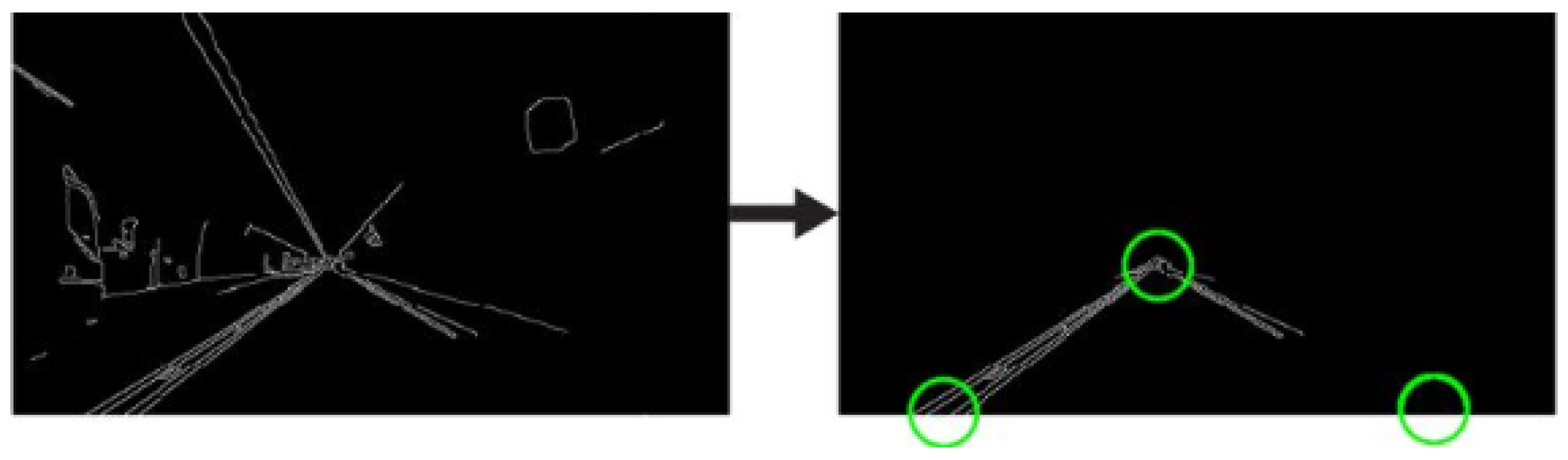
The output of the canny edge detection function is shown in Figure 2. - Region of interest (segmentation): This step takes into account only the region covered by the road lane and the image is divided into segments for processing [47]. A mask is created in this ROI. Furthermore, a bit-wise AND operation is performed between each pixel of the canny image and this mask [48]. This function masks the canny edge and shows only the required polygon ROI.Python code for defining ROI:def do_segment ( frame ) :height = frame . shape [ 0 ]polygons = np . array ( [ [ ( 0 , height ) ,( 800 , height ) , ( 380 , 290 ) ] ] )mask = np . zeros_like ( frame )cv . fillPoly (mask , polygons , 255)segment = cv . bitwise_and ( frame , mask )return segmentThe output of the ROI function is shown in Figure 2.
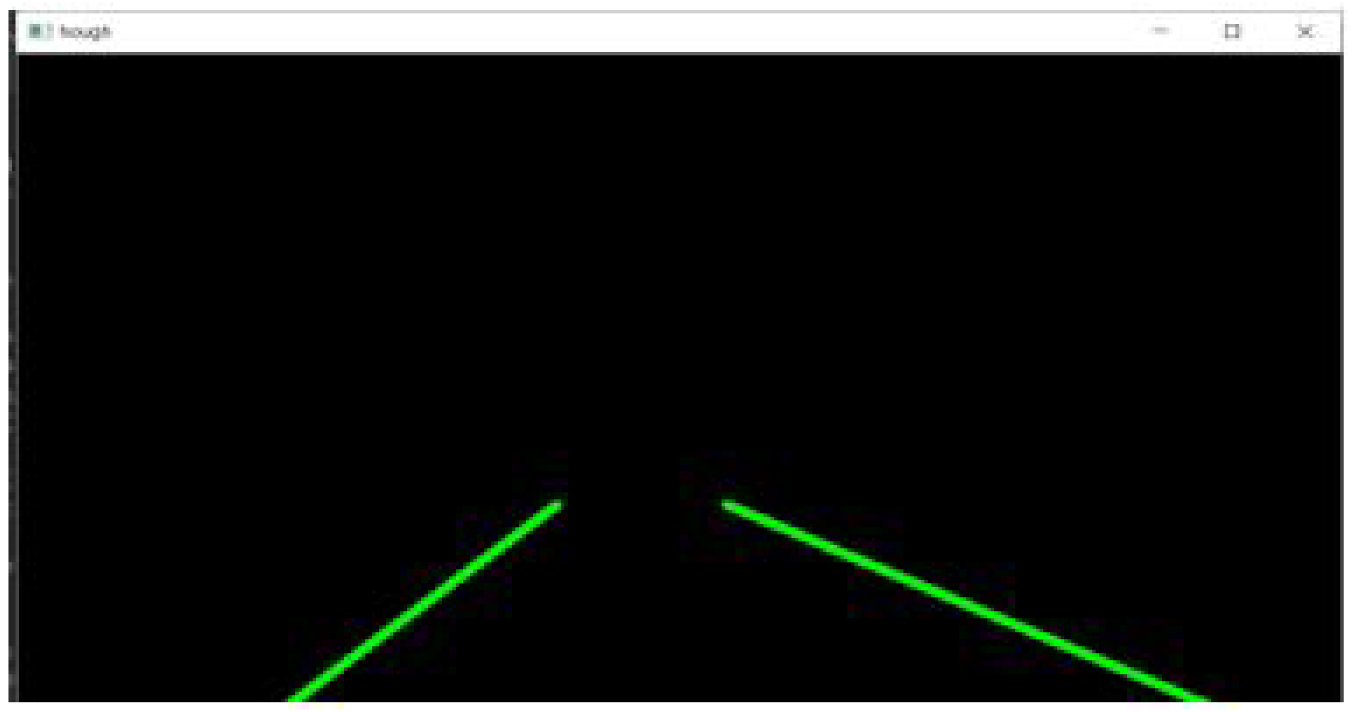
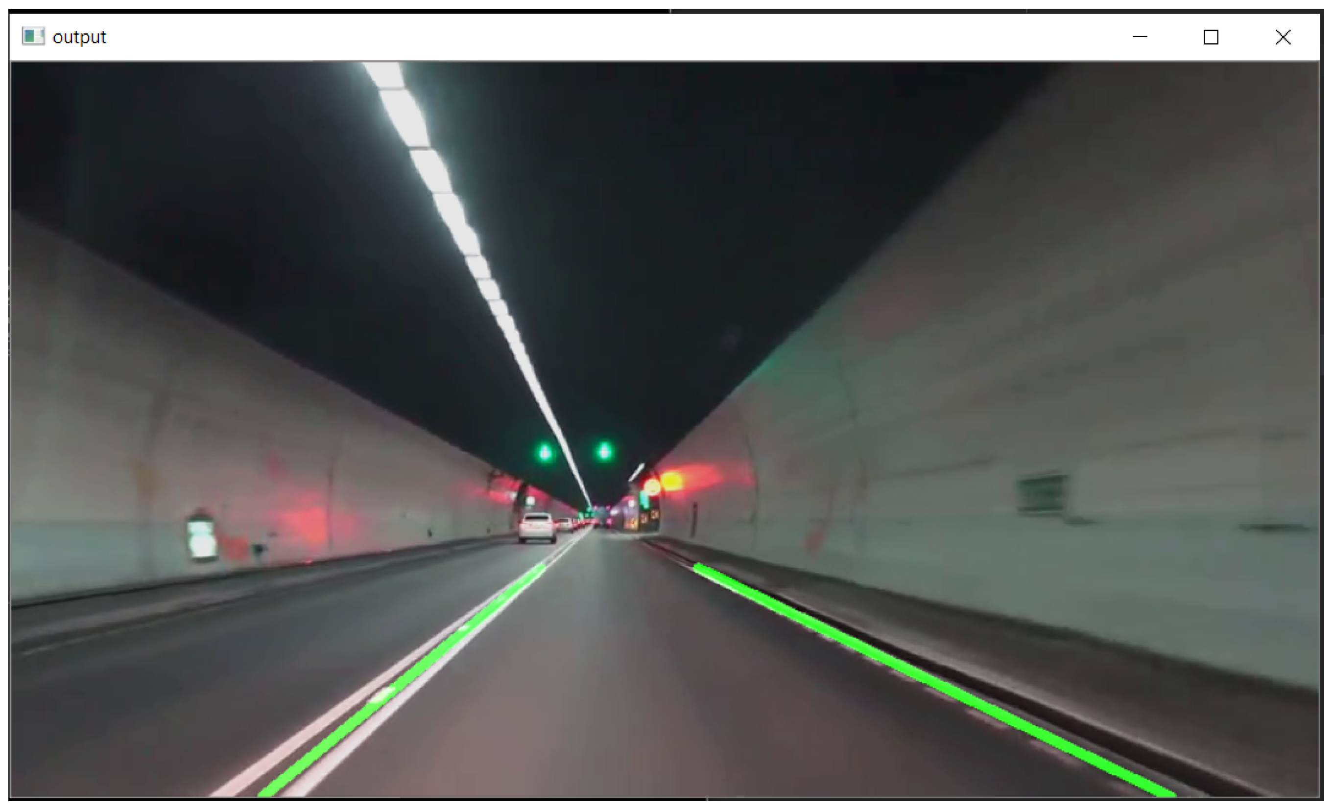
- Hough line transform: The Hough line transform [49] is a transform used to detect straight lines. The probabilistic Hough line transform is used here; this gives the extremes of the highlighted pixels of the image. This is the final step in the lane detection process and is done to find the “Lane markings” on the road. This is given mathematically byThe Hough space lines intersect at = 0.925 and r = 9.6. The curve in the polar coordinate system is given as , and a single line crossing through all these points can be given asPython code for Hough transform:hough = cv . HoughLinesP ( segment , 2 ,np . pi / 180 , 100 ,np . array ( [ ] ) , minLineLength = 100,maxLineGap = 50 )l i n e s = c a l c u l a t e_l i n e s ( frame , hough )
4.2. Case Study 2: Detection of Curved Lane Roads Using OpenCV
Case study 2 detects the curved lane using OpenCV [3]. This study mainly addresses how curved road lanes can be detected. As opposed to case study 1 which uses Hough line transforms, the same algorithm cannot be used to detect curved lanes as they usually only apply to straight lines and lanes. This section includes a number of steps. Firstly, the camera’s distortion is corrected to obtain a distinct sky view of the same image, and then this perspective is changed to obtain an image as viewed from a vehicle. Then, the colour filters are applied to the image to reduce errors and to differentiate between the usual yellow and red markings on lanes, which usually differentiate curved and straight roads. Then, a curve is fitted to the weighted pixel data, and the curved lane is obtained. These steps are explained in more detail below.
- Correcting the camera’s distortion: This involves undistorting the camera view to obtain a distinct sky view and vehicle views of the road ahead. The main cause of the change in size and shape of an object is mainly because of image distortion while being captured. This leads to a major problem: the object may appear to be closer or farther away than it actually is. All the distortion image data points can be extracted by theoretically comparing them to the actual data points which can be calculated. This is done by calling the pickle function, which is shown by the Python code below:def undistort ( img , cal_dir=r’cal_pickle . p’ ):with open ( cal_dir, mode=’rb’ ) as f :file = pickle . load ( f )mtx = file [ ’mtx’ ]dist = file [ ’dist’ ]dst = cv2 . undistort ( img , mtx , dist ,None , mtx )return dst
- Changing the perspective: The sky view perspective (bird’s eye view) is transformed into the vehicle view. For extracting all the image information, location coordinates are used to wrap the image from the calculated sky view to the required vehicle view. This is necessary because the further functions, such as applying colour filters and Sobel operators, are required to process the vehicle’s perspective view [50].
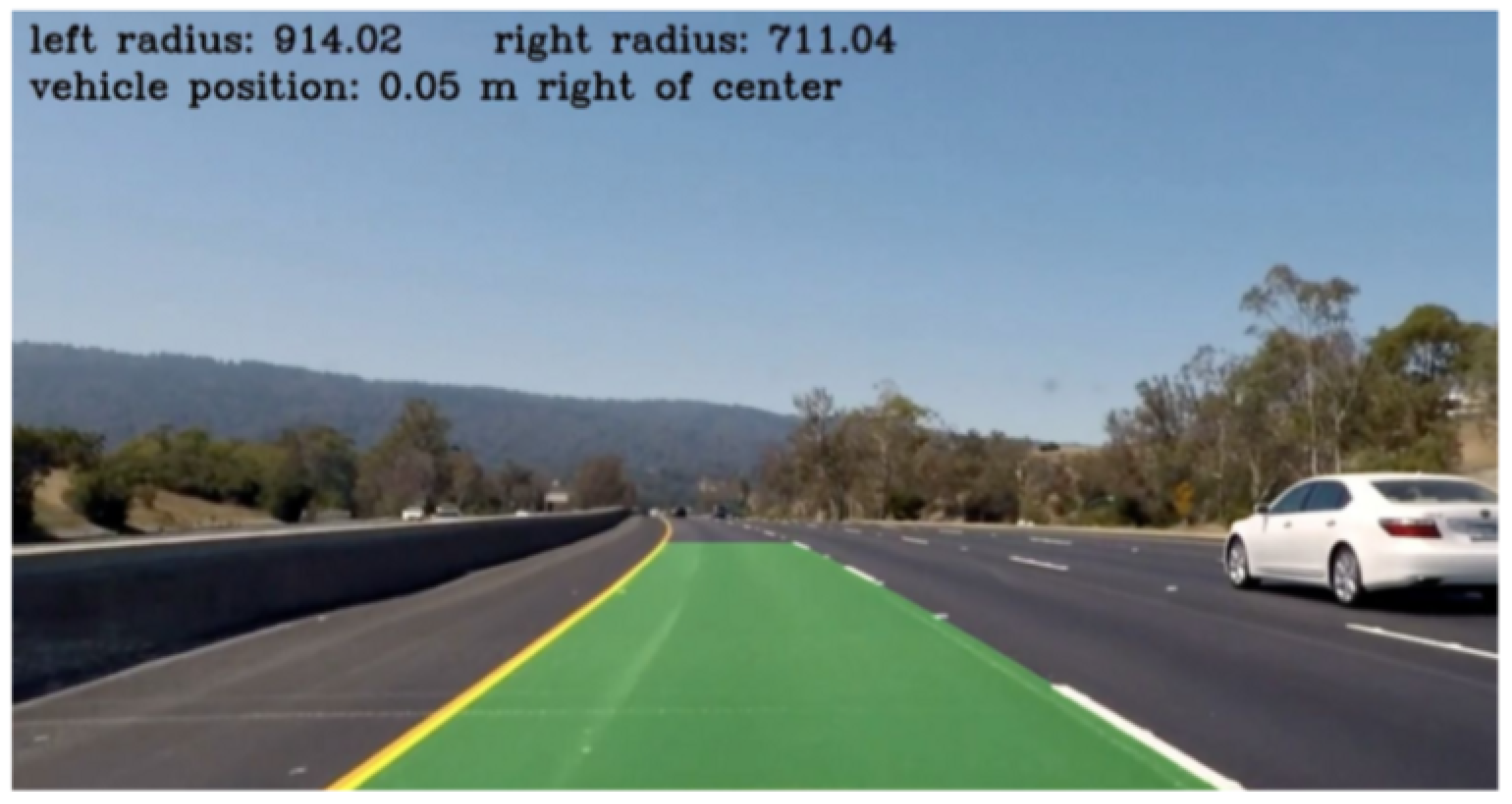
- Applying colour filters: The defined pixel values present in the ROI polygon are enough to calculate the curvature of the road. As an added precaution, there might be an error in distinguishing certain yellow and white markings on the lanes which may not actually be lanes, but markings to denote something else. In order to distinguish this, the filter mainly uses the Sobel operator [50]. The Sobel operator works by calculating the gradient of image intensity in the pixels present in the image. It is observed that this operator is very useful during the assessment of the maximum change of intensity from a lighter pixel to a darker pixel. It also helps to calculate the rate of change in the direction. It also emphatically shows how abruptly or smoothly the image changes at each pixel and how correctly the pixel represents an edge [51].The hue, saturation, and value (HSV) is a colour model that is often used in place of the RGB colour model for image processing. While using this, a specified colour value is added with a white or black contrast biasing. This can also be called hue, saturation, and brightness (HSB) [52].RGB conversion:Hue calculation:Saturation calculation:Value calculation is given bydef colorFilter ( img ):hsv = cv2 . cvtColor ( img ,cv2 . COLOR_BGR2HSV)lowerYellow = np . array ( [ 18 , 94 , 140 ] )upperYellow = np . array ( [ 48 , 255 , 255 ] )lowerWhite = np . array ( [ 0 , 0 , 200 ] )upperWhite = np . array ( [ 255 , 255 , 255 ] )maskedWhite= cv2 . inRange ( hsv ,lowerWhite , upperWhite )maskedYellow = cv2 . inRange\\(hsv,lowerYellow , upperYellow )combinedImage = $cv2 . bitwise_or$\\(maskedWhite , maskedYellow)return combinedImageA curve is fit for each line by using a second degree polynomial equation which is of the form , where A, B, and C are coefficients and are estimated by repeated trials of fitting the curve [53]. Then, the points which fit the curve the best are fed, and the curve is realized. Then, this curve is projected to the corresponding vehicle view, which is explained in the perspective transformation section. The program also gives the radius of curvature of the curved road. The output is shown in Figure 5.
4.3. Case Study 3: Behaviour Planning and Safe Lane Change Prediction Systems
Case study 3 provides the behaviour planning and safe lane change prediction systems using optimistic planning for deterministic systems (OPD) algorithms and reinforcement learning [15]. An optimal problem of a Markov decision process (MDP) with a known reward function (R -Function) is considered [15,54] and is subject to unknown deterministic dynamics, as shown in the following optimisation problem:
This MDP has several properties, which justifies using model-based reinforcement learning (MRLs) methods. The policy value is highly dependent on the goal, which adds a significant level of complexity to a model-free learning process, whereas the dynamics are completely independent of the goal and hence can be simpler to learn [11]. In the context of an industrial application, one can reasonably expect for safety concerns that the planned trajectory is required to be known in advance, before execution. To solve the abovementioned problem, MRL consists of two phases which are described in subsequent subsections.
4.3.1. Phase 1: Model Learning Phase
In the model learning phase, important input parameters are collected and used for training the model. This trained model is then tested on a validation dataset to further fine-tune the hyper parameters and measure the model’s accuracy. If the trained model is not at the required accuracy level, more data points are included in the validation set to further tune the parameters. A model is constructed and trained on the dynamics through repeated regressions on the interaction data. This is mainly done in five consecutive steps, which is explained in detail below.
- Experience collection:This randomly interacts with the environment to produce a batch of experience, which is quantified as shown in the equation below:
- Building a dynamics model:This dynamic model uses a structured model which is derived from linear time-invariant (LTI) systems. This model can be represented by the equation below:where (x, u) denotes the state and action. Intuitively, each point is obtained (, ), as well as the linearization of the true dynamics f with respect to (x, u). The next step involves parameterizing A and B as two fully connected networks with one hidden layer.
- Fit the model on the validation and training dataset:The built dynamic model (f) is trained in a supervised fashion to minimise the loss over the experience batch (D) by using stochastic gradient descent, i.e., one example at a time for 2000 epochs, as shown in Figure 6. As there is only one training set, as the number of epochs increased, the validation error also increased (above 2000), which indicated over fitting of the data. Thus, to avoid this, the number of epochs is set to be 2000, since, higher than this, an increased deviation in the validation dataset compared to the training dataset was observed.
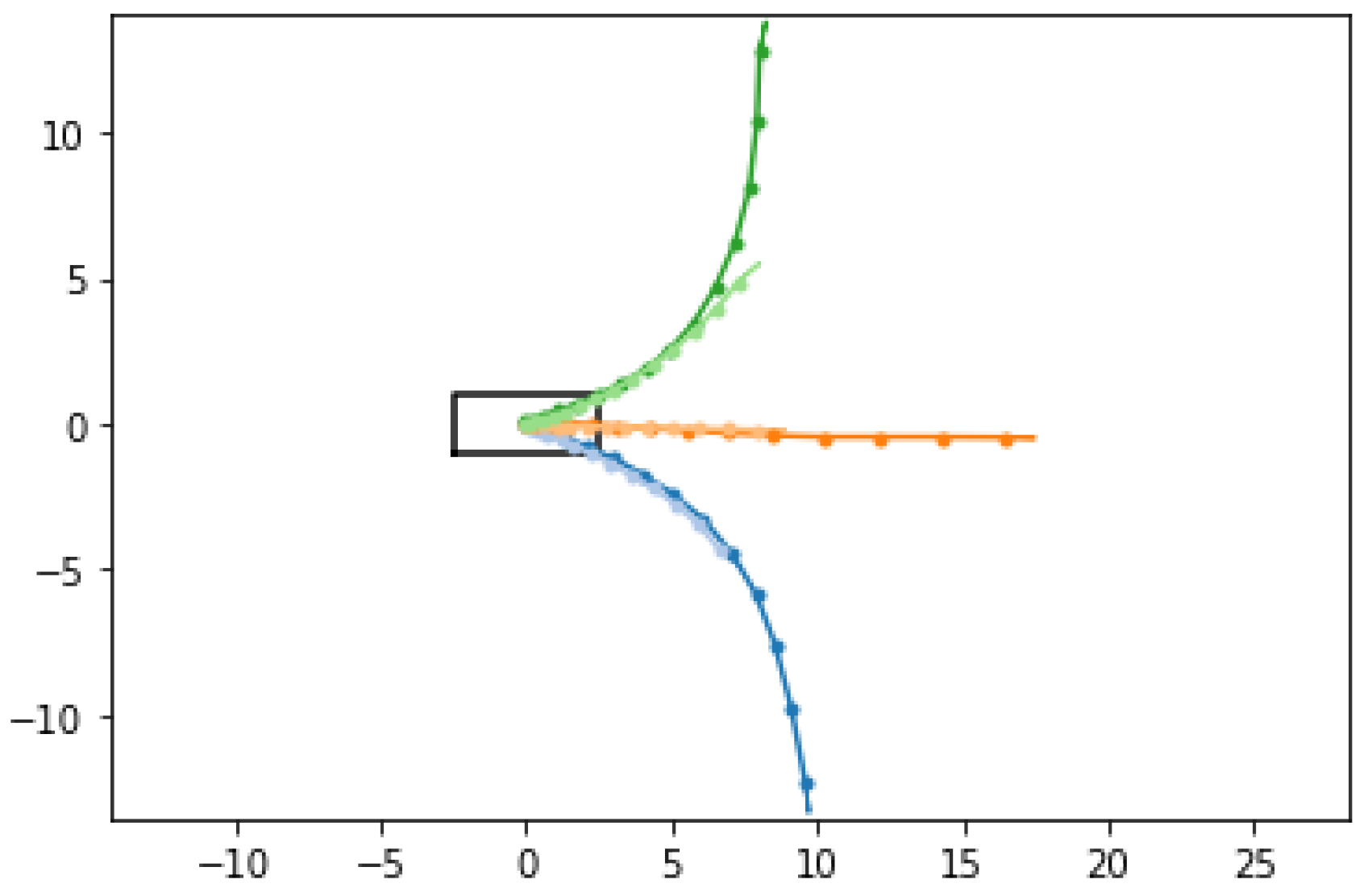
- Visualising trained dynamics and trajectories:In order to qualitatively evaluate the above-trained dynamic model (f), the values of the steering angle (such as right, centre, left) and acceleration (slow, fast) must be defined in order to predict and visualize the corresponding trajectories from an initial state, as shown in Figure 7.
- Reward model: Here, it is assumed that the reward R(s, a) is known (chosen by the system designer) and takes the form of a weighted L1-norm between the state and the goal. The simulation considers the reward of a sample transition: tensor([−0.4329]).
4.3.2. Phase 2: Planning Phase
The planning phase uses the finely tuned and trained dynamics model from the model learning phase for simulating the heterogeneous environments. In order to solve the optimal control problem, a sampling-based optimization algorithm, which is the cross entropy method, is used. The algorithm is applicable to the model learning problems, which are both combinatorial and continuous, and it is applicable to the case of finding the best performing sequence of actions. This method approximates the optimal importance sampling estimator by repeating the following two phases:
- Drawing the samples from a probability distribution which uses Gaussian distributions over the sequence of actions.
- Minimizing the cross-entropy [55] between the given and the target distribution to better the sample in the next distribution.
This distribution is compared with the given target distribution. The target distribution is defined by selecting the top performing sampled sequences. After reducing the entropy to the required level, the trained model is simulated in three different environments, such as a highway, merging of lanes on a highway, and a roundabout. The rendering of these environments is done using Pygame, and the required graphics are designed and scaled as required, finally importing the required modules for the environments, agents, and visualisation. The abovementioned environments are simulated with these defined parameters, as in Table 1 and Table 2 and are discussed as follows:
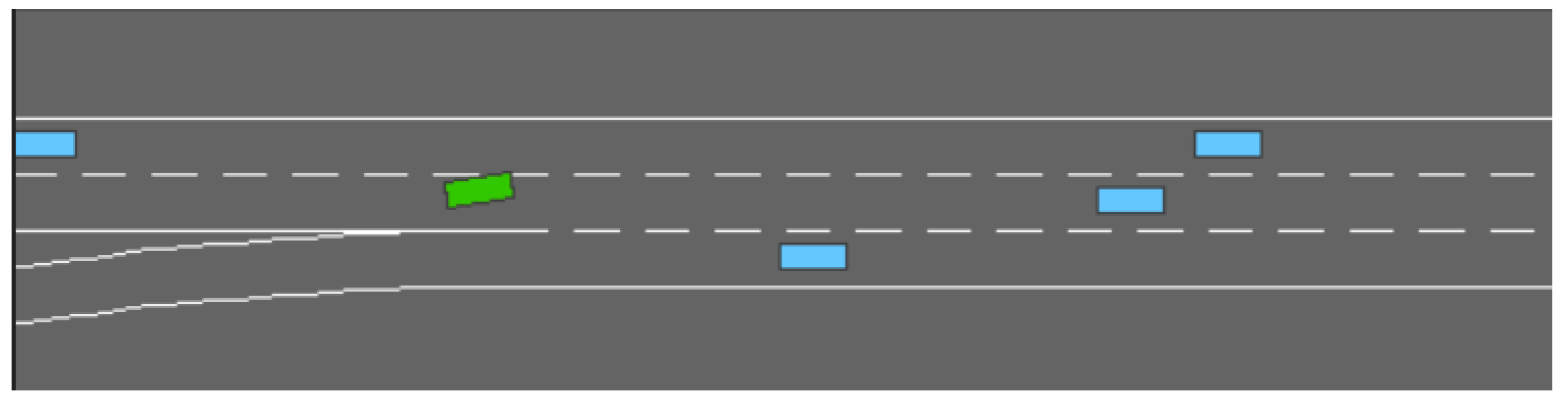
- HighwayIn the highway environment, the ego vehicle (indicated in green as shown in Figure 8) is being driven on a four-lane, one-way highway with all incoming vehicles in the same direction. The main objective of the optimisation algorithm here is to find the most optimal speed and also avoid possible collisions with the neighbouring incoming vehicles. Driving in the right lane of the road is rewarded by the reward function (as discussed in MRL phase).
- Merging of lanesIn this environment, the ego vehicle initially starts on the main highway, and an access or a service road is joined with the main highway, along with its incoming vehicles. In this environment, the main objective of the optimisation algorithm is to maintain the most optimal speed, making space and avoiding collisions with the incoming vehicles from the service lane, as shown in Figure 9.
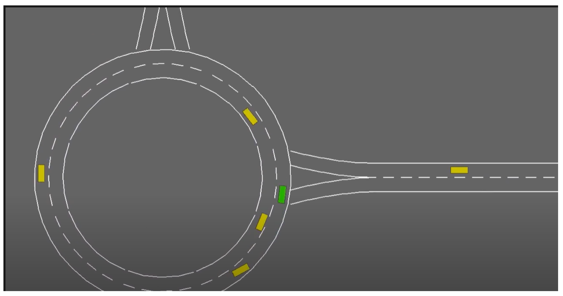
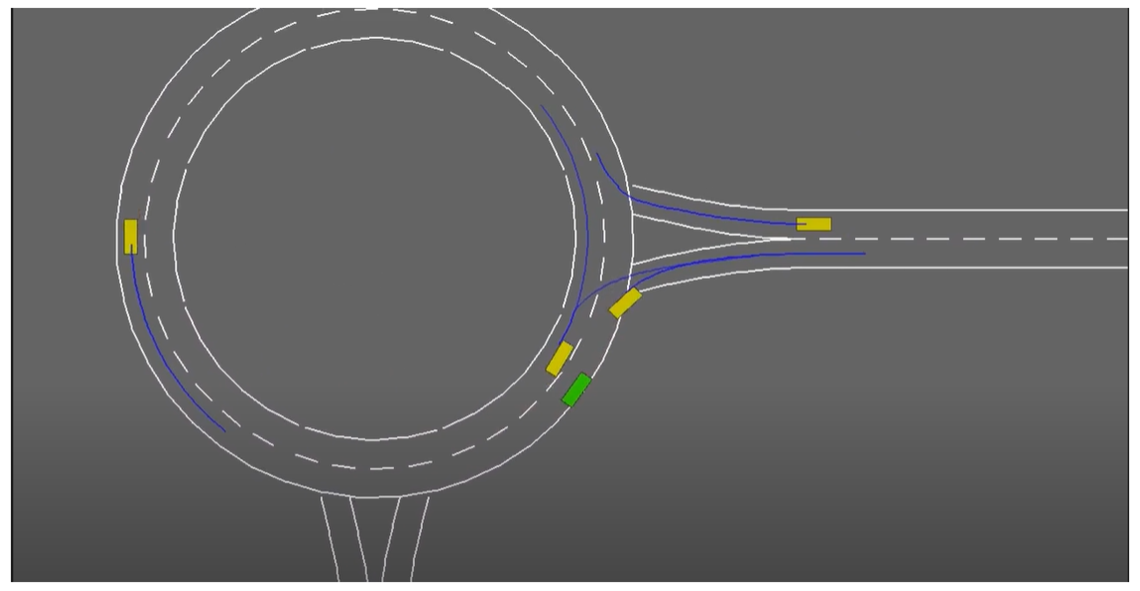
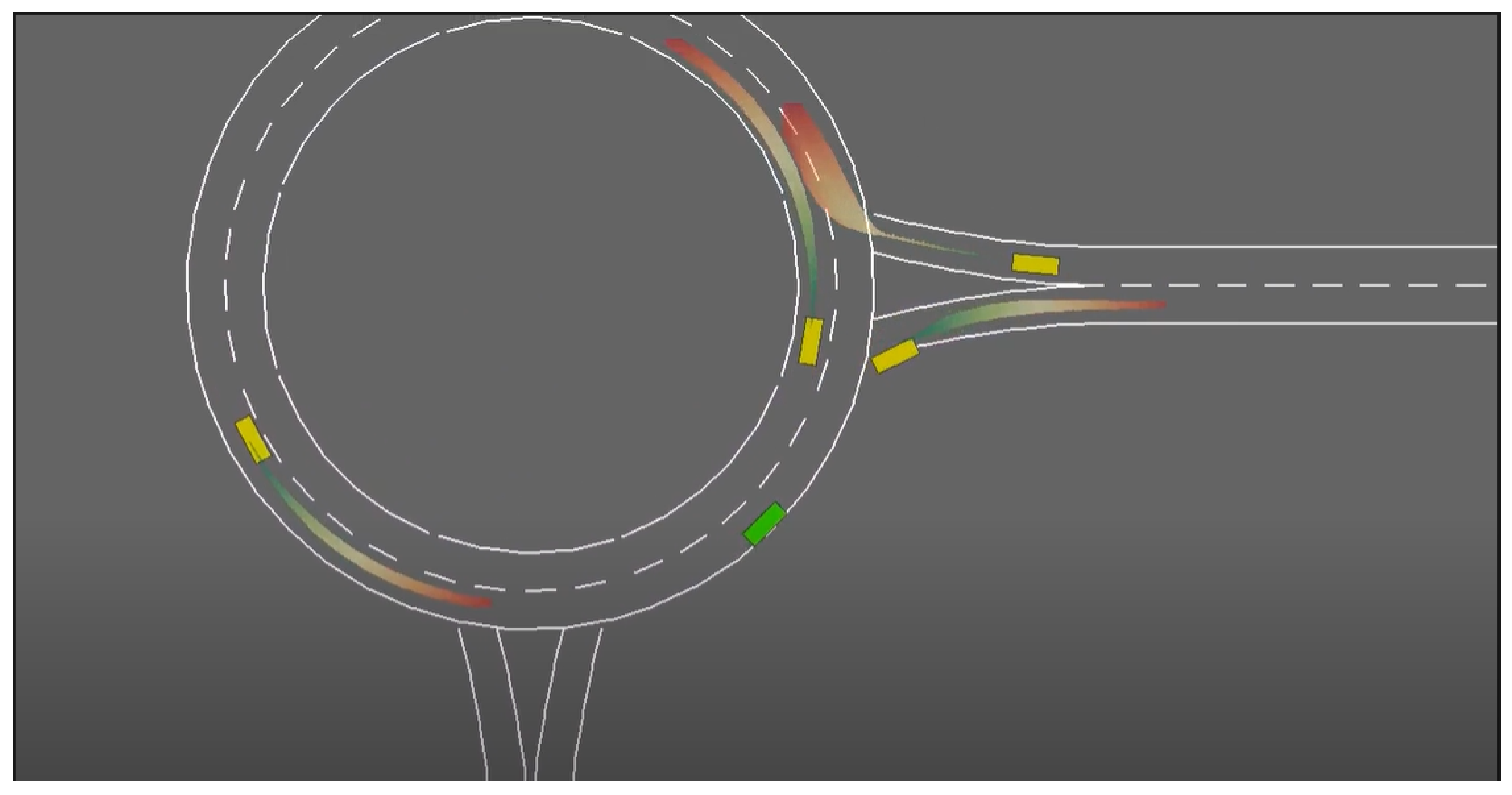
- RoundaboutIn this environment, the ego vehicle is approaching and negotiating a roundabout circle with four incoming roads. In this case, the function of the optimisation algorithm is to maintain the most optimal speed, to avoid all possible collisions within the roundabout, and to make space for the incoming vehicles from the connecting road. To optimise it further, optimum planning with the oracle model is applied, as shown in Figure 10. The oracle model utilizes the system constraints and related behaviours which may result in dangerous behaviours.The slight model errors in the oracle model can lead to catastrophic accidents and crashes, as shown in Figure 11. This occurs because the optimisation is not calibrated to the probability of the trajectory that the surrounding or adjacent vehicles can take. It affects the ego vehicle, as it ignores the trajectory of surrounding vehicles even when it is predictable.In order to account for this model’s uncertainty, a robust control framework is implemented, as shown in Figure 12, to maximise the worst case performance with respect to a set of possible behaviours, which is done by considering every possible direction that the traffic participants can take at their next intersection.It is important to take into consideration the driving styles and behaviour of the traffic participants, and this can be implemented by the robust planning with continuous ambiguity. It continuously “predicts” the trajectory of the adjacent vehicles while also considering their driving styles, as shown in Figure 13.
5. Further Studies and Scope
While the concept of autonomous vehicles has been presented for decades [12], it is only in the last five years that AVs have come into the limelight, with model cars being in physical testing phases. This is further growing due to increased demand for self-driving cars which increase traffic safety, but currently, full autonomous driving technology has been restricted only to logistics and shuttle services with defined and familiar paths [6]. This is mainly due to safety issues arising from the potential threat of welcoming a nascent technology onto roads with driver-driven vehicles, where safety concerns may arise, as some ‘autonomous’ driving technologies can only respond to limited situations. However, in the near future, with highly responsive and accurate neural networks and decision-making algorithms and systems, it is believed that AVs will be an indispensable part of transportation systems [56,57]. The integration of AVs into society would only be complete if the driver/passenger could completely and comfortably trust the vehicle to drive itself safely. This can be achieved by comprehensive public demonstrations, by placing AVs in various hazardous scenarios and showcasing their responses to numerous ‘unpredictable’ situations–at least by human standards–which can be statistically predicted by vehicle on-board computers [58]. This was effectively done by Tesla, which successfully demonstrated this on the company’s ‘Autonomy Day’ event, where various drives and accident and response scenarios where showcased. Tesla also showcased its easier to use user interface (UI) for autonomous driving, which would enable drivers to easily visualise the vehicle’s surroundings, thereby reducing the possibility of accidents [58]. Similar advancements are being observed for numerous other automotive companies, which are focusing on AV development. Additionally, the advancement of machine learning and neural networks can bring far reaching contributions to increasing the precision of autonomous driving, in particular with the introduction of the concept of neuroplasticity [59]. Finally, with the coupling of technology in urban fabrics, leading to the advancement of the concept of smart cities [60,61,62] and the need for more compact yet connected neighbourhoods [63], it is expected that sensors will be able to further communicate with AVs, resulting in even safer driving experiences. This is even expected to be facilitated by upcoming 6G technologies [64]. These advancements warrant further research and development of safer and more proactive AV systems that can surely match or surpass a human driver in safe and secure driving.
In regards to the current study, specific methods for addressing problems related to lane detection (both straight and curved lanes) were proposed by using Hough transforms and HSV conversions and simulated by MDP algorithms for behavioural planning, enabling vehicles to manoeuvre accurately by estimating the states of surrounding vehicles. A shortcoming of the MDP model was recognised and accordingly addressed, and it is to be noted that this method is highly case specific, as it takes into account only the surrounding vehicles and not other factors such as people, animals, etc. These would be highly complex to model, as this state estimation cannot be applied to people. In future research, this can be addressed by building prediction models for human behaviour on roads and also modelling human and vehicle interactions. These simulations could then be combined to render a more realistic scenario which includes people’s behaviours.
6. Conclusions
This paper thoroughly discusses the safety and risk measures and analysis of autonomous vehicles through the developed dynamic run-time safe assessment system to understand how a variation in the ODD could affect the operation of AVs, so that vehicles could remain operational in safe mode, which is explored via different scenarios and factors. In particular, a CCA approach to manoeuvre through incoming vehicles is adopted and discussed, with test cases for V2X communication, via an ’elastic band’ method, and decision-making algorithms, for lane changing and straight lines via Hough transforms. A contribution of this paper is the modification of the Hough transform algorithm to allow AVs to detect curved lanes, which is achieved by removing captured image distortions by capturing a colour matrix of the image, hence deriving the radius of the curvature of the road.
Case studies, via an ego vehicle through the use of MRLs, were performed as part of the analysis, where the algorithm was tested in two phases over 2000 epochs to reduce the variance between the validation and training datasets. Furthermore, the planning phase oversaw the ego vehicle’s manoeuvrability, where the MDP algorithm was tested in three environments: velocity variance, lane changing, and lane merging.
With the application of a robust control framework, it was noted that the ego vehicle was able to predict the states of its surrounding vehicles, hence gaining the ability to predict the possible paths of surrounding vehicles. It is noted that there is no single pathway towards achieving autonomous driving, where a multitude of methods may be utilised. However, human safety should be optimised at all levels, where AV companies should prioritise this aspect, which will then lead to increased adoption and subsequently the further development of the concept.
Author Contributions
Conceptualization, Methodology, Software, Formal Analysis, Investigation, and Visualization by A.D.; Validation by A.D.; Data Curation by R.K.C.; Writing—Original Draft Preparation by A.D.; Writing—Review and Editing by A.D. and Z.A.; Supervision by Z.A. All authors have read and agreed to the published version of the manuscript.
Funding
This research received no external funding.
Institutional Review Board Statement
Not applicable.
Informed Consent Statement
Not applicable.
Data Availability Statement
Not applicable.
Conflicts of Interest
The authors declare no conflict of interest.
Nomenclature
| Symbol | Quantity |
| S | Given set of states |
| A | The action state |
| O | The observation space |
| Z | The uncertainty of the sensor reading |
| T | The uncertainty of the system dynamics and the surrounding environment |
| R | The optimum function produced for the state known as the reward function |
| The discount factor which is in the range of [0,1) | |
| X2 | The end position of ego vehicle |
| X1 | The initial position of the neighbouring vehicle |
| Vajd | The velocity of the neighbouring vehicle |
| Vego | The velocity of the ego vehicle |
| Tmanoeuvre | The time it takes to finish the manoeuvre |
| Xsafety | The additional safety distance for extra tolerance |
| r | Radius of curvature of the road |
| Angle between the intersected Hough lines | |
| Final internal force between the ith and (i + 1)th elastic band node | |
| Initial internal force between the ith and (i + 1)th elastic band node | |
| Displacement of the ith knot | |
| Displacement of the i + 1th knot | |
| Displacement of the i − 1th knot | |
| ks | Spring constant in the range (0, 1] |
| External force acting at the ith node element |
References
- SAE International Releases Updated Visual Chart for Its “Levels of Driving Automation” Standard for Self-Driving Vehicles. Available online: https://www.sae.org/news/press-room/2018/12/sae-international-releases-updated-visual-chart-for-its-%E2%80%9Clevels-of-driving-automation%E2%80%9D-standard-for-self-driving-vehicles (accessed on 15 December 2020).
- Rathour, S.S.; Ishigooka, T.; Otsuka, S.; MARTIN, R. Runtime Active Safety Risk-Assessment of Highly AutonomousVehicles for Safe Nominal Behavior; SAE Technical Paper 2020-01-0107; SAE International: Seville, Spain, 2020. [Google Scholar] [CrossRef]
- Udacity’s Self Driving Nano Degree Programme. Available online: https://www.udacity.com/course/self-driving-car-engineer-nanodegree--nd013 (accessed on 15 November 2020).
- Kukkala, V.K.; Tunnell, J.; Pasricha, S.; Bradley, T. Advanced Driver-Assistance Systems: A Path Toward Autonomous Vehicles. IEEE Consum. Electron. Mag. 2018, 7, 18–25. [Google Scholar] [CrossRef]
- Gelbal, S.Y.; Zhu, S.; Anantharaman, G.A.; Guvenc, B.A.; Guvenc, L. Cooperative Collision Avoidance in a Connected Vehicle Environment; SAE Technical Paper 2019-01-0488; SAE International: Warrendale, PA, USA, 2019. [Google Scholar] [CrossRef]
- Nugraha, B.T.; Su, S.F. Towards self-driving car using convolutional neural network and road lane detector. In Proceedings of the 2017 2nd International Conference on Automation, Cognitive Science, Optics, Micro Electro–Mechanical System, and Information Technology (ICACOMIT), Jakarta, Indonesia, 23–24 October 2017; pp. 65–69. [Google Scholar] [CrossRef]
- Latham, A.; Nattrass, M. Autonomous vehicles, car-dominated environments, and cycling: Using anethnography of infrastructure to reflect on the prospects of a newtransportation technology. J. Transp. Geogr. 2019, 81, 102539. [Google Scholar] [CrossRef]
- Brechtel, S.; Gindele, T.; Dillmann, R. Probabilistic Decision-Making under Uncertainty for Autonomous Driving Using Continuous POMDP. In Proceedings of the IEEE 17th International Conference on Intelligent Transportation Systems (ITSC), Qingdao, China, 8–11 October 2014. [Google Scholar] [CrossRef]
- Berns, K. Off-road robotics-perception and navigation. In Proceedings of the 2014 11th International Conference on Informatics in Control, Automation and Robotics (ICINCO), Vienna, Austria, 1–3 September 2014; pp. IS-9–IS-11. [Google Scholar]
- Berecz, C.E.; Kiss, G. Dangers in autonomous vehicles. In Proceedings of the 2018 IEEE 18th International Symposium on Computational Intelligence and Informatics (CINTI), Budapest, Hungary, 21–22 November 2018; pp. 000263–000268. [Google Scholar] [CrossRef]
- Wei, J.; Dolan, J.M.; Snider, J.M.; Litkouhi, B. A point-based MDP for robust single-lane autonomous driving behavior under uncertainties. In Proceedings of the 2011 IEEE International Conference on Robotics and Automation, Shanghai, China, 9–13 May 2011; pp. 2586–2592. [Google Scholar] [CrossRef]
- Pressman, A. Waymo Reaches 20 Million Miles of Autonomous Driving. Fortune. 7 January 2020. Available online: https://fortune.com/2020/01/07/googles-waymo-reaches-20-million-miles-of-autonomous-driving/ (accessed on 8 July 2020).
- Colwell, I.; Phan, B.; Saleem, S.; Salay, R.; Czarnecki, K. An Automated Vehicle Safety Concept Based on Runtime Restriction of the Operational Design Domain. In Proceedings of the 2018 IEEE Intelligent Vehicles Symposium (IV), Changshu, China, 26–30 June 2018; pp. 1910–1917. [Google Scholar] [CrossRef]
- Korosec, K. Watch a Waymo Self-Driving Car Test Its Sensors in a Haboob. Techcrunch. 23 August 2019. Available online: https://techcrunch.com/2019/08/23/watch-a-waymo-self-driving-car-test-its-sensors-in-a-haboob/ (accessed on 2 August 2020).
- Highway-Env, Leurent, Edouard, An Environment for Autonomous Driving Decision-Making, GitHub, GitHub Repository. 2018. Available online: https://github.com/eleurent/highway-env (accessed on 12 September 2020).
- Anaya, J.J.; Merdrignac, P.; Shagdar, O.; Nashashibi, F.; Naranjo, J.E. Vehicle to pedestrian communications for protection of vulnerable road users. In Proceedings of the 2014 IEEE Intelligent Vehicles Symposium Proceedings, Dearborn, MI, USA, 8–11 June 2014; pp. 1037–1042. [Google Scholar] [CrossRef] [Green Version]
- SAE Standards News J3016 Automated-Driving Graphic Update 2019-01-07 JENNIFER SHUTTLEWORTH SAE Updates J3016 Levels of Automated Driving Graphic to Reflect Evolving Standard. Available online: https://www.sae.org/news/2019/01/sae-updates-j3016-automated-driving-graphic (accessed on 12 September 2020).
- Shuttleworth, J. SAE Standards News: J3016 Automated-Driving Graphic Update. 7 January 2019. Available online: https://www.sae.org/news/2019/01/sae-updates-j3016-automated-driving-graphic (accessed on 16 October 2020).
- Gnatzig, S.; Schuller, F.; Lienkamp, M. Human-machine interaction as key technology for driverless driving-A trajectory-based shared autonomy control approach. In Proceedings of the 2012 IEEE RO-MAN: The 21st IEEE International Symposium on Robot and Human Interactive Communication, Paris, France, 9–13 September 2012; pp. 913–918. [Google Scholar] [CrossRef]
- Al Zamil, M.G.; Samarah, S.; Rawashdeh, M.; Hossain, M.S.; Alhamid, M.F.; Guizani, M.; Alnusair, A. False-Alarm Detection in the Fog-Based Internet of Connected Vehicles. IEEE Trans. Veh. Technol. 2019, 68, 7035–7044. [Google Scholar] [CrossRef]
- Qian, Y.; Chen, M.; Chen, J.; Hossain, M.S.; Alamri, A. Secure Enforcement in Cognitive Internet of Vehicles. IEEE Internet Things J. 2018, 5, 1242–1250. [Google Scholar] [CrossRef]
- Nanda, A.; Puthal, D.; Rodrigues, J.J.P.C.; Kozlov, S.A. Internet of Autonomous Vehicles Communications Security: Overview, Issues, and Directions. IEEE Wirel. Commun. 2019, 26, 60–65. [Google Scholar] [CrossRef]
- Jameel, F.; Chang, Z.; Huang, J.; Ristaniemi, T. Internet of Autonomous Vehicles: Architecture, Features, and Socio-Technological Challenges. IEEE Wirel. Commun. 2019, 26, 21–29. [Google Scholar] [CrossRef] [Green Version]
- Qian, Y.; Jiang, Y.; Hu, L.; Hossain, M.S.; Alrashoud, M.; Al-Hammadi, M. Blockchain-Based Privacy-Aware Content Caching in Cognitive Internet of Vehicles. IEEE Netw. 2020, 34, 46–51. [Google Scholar] [CrossRef]
- Chou, F.; Shladover, S.E.; Bansal, G. Coordinated merge control based on V2V communication. In Proceedings of the 2016 IEEE Vehicular Networking Conference (VNC), Columbus, OH, USA, 8–10 December 2016; pp. 1–8. [Google Scholar] [CrossRef]
- Nie, J.; Zhang, J.; Ding, W.; Wan, X.; Chen, X.; Ran, B. Decentralized Cooperative Lane-Changing Decision-Making for Connected Autonomous Vehicles*. IEEE Access 2016, 4, 9413–9420. [Google Scholar] [CrossRef]
- Qian, S.; Zhang, T.; Xu, C.; Hossain, M.S. Social event classification via boosted multimodal supervised latent dirichlet allocation. ACM Trans. Multimed. Comput. Commun. Appl. 2015, 11, 27.1–27.22. [Google Scholar] [CrossRef]
- Yang, X.; Zhang, T.; Xu, C.; Hossain, M.S. Automatic Visual Concept Learning for Social Event Understanding. IEEE Trans. Multimed. 2015, 17, 346–358. [Google Scholar] [CrossRef]
- Norman, G.; Parker, D.; Zou, X. Verification and control of partially observable probabilistic systems. Real-Time Syst. 2017, 53, 354–402. [Google Scholar] [CrossRef] [Green Version]
- Bouton, M.; Cosgun, A.; Kochenderfer, M.J. Belief state planning for autonomously navigating urban intersections. In Proceedings of the 2017 IEEE Intelligent Vehicles Symposium (IV), Los Angeles, CA, USA, 11–14 June 2017; pp. 825–830. [Google Scholar] [CrossRef] [Green Version]
- Babu, M.; Oza, Y.; Singh, A.K.; Krishna, K.M.; Medasani, S. Model Predictive Control for Autonomous Driving Based on Time Scaled Collision Cone. In Proceedings of the 2018 European Control Conference (ECC), Limassol, Cyprus, 12–15 June 2018; pp. 641–648. [Google Scholar] [CrossRef] [Green Version]
- Mizushima, Y.; Okawa, I.; Nonaka, K. Model Predictive Control for Autonomous Vehicles with Speed Profile Shaping. IFAC-PapersOnLine 2019, 52, 31–36. [Google Scholar] [CrossRef]
- Yurtsever, E.; Lambert, J.; Carballo, A.; Takeda, K. A Survey of Autonomous Driving: Common Practices and Emerging Technologies. IEEE Access 2020, 8, 58443–58469. [Google Scholar] [CrossRef]
- Lertniphonphan, K.; Komorita, S.; Tasaka, K.; Yanagihara, H. 2D to 3D Label Propagation For Object Detection In Point Cloud. In Proceedings of the 2018 IEEE International Conference on Multimedia and Expo Workshops (ICMEW), San Diego, CA, USA, 23–27 July 2018; pp. 1–6. [Google Scholar] [CrossRef]
- Hu, X.; Xu, X.; Xiao, Y.; Chen, H.; He, S.; Qin, J.; Heng, P.A. SINet: A Scale-Insensitive Convolutional Neural Network for Fast Vehicle Detection. IEEE Trans. Intell. Transp. Syst. 2019, 20, 1010–1019. [Google Scholar] [CrossRef] [Green Version]
- Yang, X.; Zhang, T.; Xu, C.; Yan, S.; Hossain, M.S.; Ghoneim, A. Deep Relative Attributes. IEEE Trans. Multimed. 2016, 18, 1832–1842. [Google Scholar] [CrossRef]
- Pan, X.; Shi, J.; Luo, P.; Wang, X.; Tang, X. Spatial as Deep: Spatial CNN for Traffic Scene Understanding. The Chinese University of Hong Kong. SenseTime Group Limited. Available online: https://www.aaai.org/ocs/index.php/AAAI/AAAI18/paper/viewFile/16802/16322 (accessed on 11 January 2021).
- Liu, R.W.; Nie, J.; Garg, S.; Xiong, Z.; Zhang, Y.; Hossain, M.S. Data-Driven Trajectory Quality Improvement for Promoting Intelligent Vessel Traffic Services in 6G-Enabled Maritime IoT Systems. IEEE Internet Things J. 2020, 8, 5374–5385. [Google Scholar] [CrossRef]
- Lee, J.; Park, S. New interconnection methodology of TSNs using V2X communication. In Proceedings of the 2017 IEEE 7th Annual Computing and Communication Workshop and Conference (CCWC), Las Vegas, NV, USA, 9–11 January 2017; pp. 1–6. [Google Scholar] [CrossRef]
- Abou-zeid, H.; Pervez, F.; Adinoyi, A.; Aljlayl, M.; Yanikomeroglu, H. Cellular V2X Transmission for Connected and Autonomous Vehicles Standardization, Applications, and Enabling Technologies. IEEE Consum. Electron. Mag. 2019, 8, 91–98. [Google Scholar] [CrossRef]
- Gelbal, S.Y.; Arslan, S.; Wang, H.; Aksun-Guvenc, B.; Guvenc, L. Elastic band based pedestrian collision avoidance using V2X communication. In Proceedings of the 2017 IEEE Intelligent Vehicles Symposium (IV), Los Angeles, CA, USA, 11–14 June 2017; pp. 270–276. [Google Scholar] [CrossRef]
- An, H.; Jung, J.I. Design of a Cooperative Lane Change Protocol for a Connected and Automated Vehicle Based on an Estimation of the Communication Delay. Sensors 2018, 18, 3499. [Google Scholar] [CrossRef] [PubMed] [Green Version]
- Zhang, X.; Peng, M.; Yan, S.; Sun, Y. Deep-Reinforcement-Learning-Based Mode Selection and Resource Allocation for Cellular V2X Communications. IEEE Internet Things J. 2020, 7, 6380–6391. [Google Scholar] [CrossRef] [Green Version]
- Chen, L.C.; Papandreou, G.; Kokkinos, I.; Murphy, K.; Yuille, A.L. DeepLab: Semantic Image Segmentation with Deep Convolutional Nets, Atrous Convolution, and Fully Connected CRFs. arXiv 2017, arXiv:1606.00915v2. [Google Scholar] [CrossRef]
- Pan, B.; Lu, Z.; Xie, H. Mean Intensity Gradient: An Effective Global Parameter for Quality Assessment of the Speckle Patterns Used in Digital Image Correlation. Opt. Lasers Eng. 2010, 48, 469–477. [Google Scholar] [CrossRef]
- Hou, Z.; Liu, X.; Chen, L. Object Detection Algorithm for Improving Non-Maximum Suppression Using GIoU. IOP Conf. Ser. Mater. Sci. Eng. 2020, 790, 012062. [Google Scholar] [CrossRef]
- George Seif Semantic Segmentation with Deep Learning. Available online: https://towardsdatascience.com/semantic-segmentation-with-deep-learning-a-guideand-code-e52fc8958823 (accessed on 13 November 2020).
- Lee, J.; Lian, F.; Lee, H. Region Growing Approach on Detecting Drivable Space for Intelligent Autonomous Vehicles. In Proceedings of the 2018 7th International Congress on Advanced Applied Informatics (IIAI-AAI), Yonago, Japan, 8–13 July 2018; pp. 972–973. [Google Scholar] [CrossRef]
- Shehata, A.; Mohammad, S.; Abdallah, M.; Ragab, M. A Survey on Hough Transform, Theory, Techniques and Applications. arXiv 2015, arXiv:1502.02160. [Google Scholar]
- Feng, Y.; Rong-ben, W.; Rong-hui, Z. Based on Digital Image Lane Edge Detection and Tracking under Structure Environment for Autonomous Vehicle. In Proceedings of the 2007 IEEE International Conference on Automation and Logistics, Jinan, China, 18–21 August 2007; pp. 1310–1314. [Google Scholar] [CrossRef]
- Misra, S.; Yaokun, W. Machine Learning for Subsurface Characterization; Gulf Professional Publishing: Houston, TX, USA, 2020. [Google Scholar] [CrossRef]
- Najafi Kajabad, E. Detection of Vehicle and Brake Light Based on Cascade and HSV Algorithm in Autonomous Vehicle. In Proceedings of the 2018 International Conference on Industrial Engineering, Applications and Manufacturing (ICIEAM), Moscow, Russia, 15–18 May 2018; pp. 1–5. [Google Scholar] [CrossRef]
- Mithi Road Lane Lines Detection Using Advanced Computer Vision Techniques. Available online: https://medium.com/@mithi/advanced-lane-finding-using-computer-vision-techniques7f3230b6c6f2 (accessed on 10 February 2020).
- Okuyama, T.; Gonsalves, T.; Upadhay, J. Autonomous Driving System based on Deep Q Learnig. In Proceedings of the 2018 International Conference on Intelligent Autonomous Systems (ICoIAS), Singapore, 1 March 2018; pp. 201–205. [Google Scholar] [CrossRef]
- Barthelme, A.; Wiesmayr, R.; Utschick, W. Model Order Selection in DoA Scenarios via Cross-entropy Based Machine Learning Techniques. In Proceedings of the ICASSP 2020—2020 IEEE International Conference on Acoustics, Speech and Signal Processing (ICASSP), Barcelona, Spain, 4–8 May 2020; pp. 4622–4626. [Google Scholar] [CrossRef] [Green Version]
- Chavhan, S.; Gupta, D.; Garg, S.; Khanna, A.; Choi, B.J.; Hossain, M.S. Privacy and Security Management in Intelligent Transportation System. IEEE Access 2020, 8, 148677–148688. [Google Scholar] [CrossRef]
- Zhang, Y.; Li, Y.; Wang, R.; Hossain, M.S.; Lu, H. Multi-Aspect Aware Session-Based Recommendation for Intelligent Transportation Services. IEEE Trans. Intell. Transp. Syst. 2020. [Google Scholar] [CrossRef]
- Bellan, R.; Alamalhodaei, A. Top four highlights of Elon Musk’s Tesla AI Day. 20 August 2021. Available online: https://techcrunch.com/2021/08/19/top-five-highlights-of-elon-musks-tesla-ai-day/ (accessed on 12 October 2020).
- Allam, Z. Achieving Neuroplasticity in Artificial Neural Networks through Smart Cities. Smart Cities 2019, 2, 118–134. [Google Scholar] [CrossRef] [Green Version]
- Allam, Z.; Dhunny, Z.A. On big data, artificial intelligence and smart cities. Cities 2019, 89, 80–91. [Google Scholar] [CrossRef]
- Sharifi, A.; Allam, Z.; Feizizadeh, B.; Ghamari, H. Three Decades of Research on Smart Cities: Mapping Knowledge Structure and Trends. Sustainability 2021, 13, 7140. [Google Scholar] [CrossRef]
- Allam, Z. Cities and the Digital Revolution: Aligning Technology and Humanity; Springer International Publishing: Berlin/Heidelberg, Germany, 2020. [Google Scholar]
- Moreno, C.; Allam, Z.; Chabaud, D.; Gall, C.; Pratlong, F. Introducing the “15-Minute City”: Sustainability, Resilience and Place Identity in Future Post-Pandemic Cities. Smart Cities 2021, 4, 93–111. [Google Scholar] [CrossRef]
- Allam, Z.; Jones, D.S. Future (post-COVID) digital, smart and sustainable cities in the wake of 6G: Digital twins, immersive realities and new urban economies. Land Use Policy 2021, 101, 105201. [Google Scholar] [CrossRef]
Figure 1.
Operational states of ODDs.

Figure 2.
Canny edge detection and establishing the ROI.

Figure 3.
Corresponding Hough line transform.

Figure 4.
Final output of the Lane Detection Algorithm.

Figure 5.
Lane detection for curved roads.

Figure 6.
Decrease in loss function over 2000 epochs.

Figure 7.
Left, right, and centre trajectories of ego vehicle visualised after training in the X,Y plane.
Figure 7.
Left, right, and centre trajectories of ego vehicle visualised after training in the X,Y plane.

Figure 8.
Lane changing in the highway environment (ego vehicle in green).

Figure 9.
Behaviour when lanes merge. The ego vehicle makes way for the incoming vehicle from the adjacent lane.
Figure 9.
Behaviour when lanes merge. The ego vehicle makes way for the incoming vehicle from the adjacent lane.

Figure 10.
Roundabout simulation on oracle model.

Figure 11.
Accident cases due to errors in the model and inability to predict vehicle trajectories (as shown in red).
Figure 11.
Accident cases due to errors in the model and inability to predict vehicle trajectories (as shown in red).

Figure 12.
Model with robust control framework implemented.

Figure 13.
Robust control with continuous ambiguity to predict trajectories of surrounding vehicles.
Figure 13.
Robust control with continuous ambiguity to predict trajectories of surrounding vehicles.


Table 1.
Parameters and their quantitative meaning.
| Parameter | Definition |
|---|---|
| Acceleration Range | Range of acceleration of ego vehicle |
| Steering Range | Maximum and minimum steering angle of the ego vehicle |
| Actions All | Labels for all the actions performed by the ego vehicle |
| Actions Longit | Labels for the actions performed in the longitudinal plane |
| Actions Lat | Labels for the actions performed in the lateral plane |
| Max Speed | Maximum speed limit on the ego vehicle |
| Default Speeds | Default initial speed |
| Distance Wanted | Desired distance to the vehicle in front |
| Time Wanted | Time gap desired to the vehicle in front |
| Stripe Spacing | Distance between the road stripe and the edge of the road |
| Stripe Length | Length of the stripe |
| Stripe Width | Width of the stripe |
| Perception Distance | Distance the ego vehicle can perceive |
| Collisions Enabled | Ego vehicle is open for collisions which the system avoids |
Table 2.
Simulation parameters and labels for highway, merging of lanes, and roundabout environments.
Table 2.
Simulation parameters and labels for highway, merging of lanes, and roundabout environments.
| Parameter | Quantity |
|---|---|
| Acceleration Range | ms−2 |
| Steering Range | rad |
| Actions All | 0: ‘Lane Left’, 1: ‘Idle’, 2: ‘Lane Right’, 3: ‘Faster’, 4: ‘Slower’ |
| Actions Longit | 0: ‘Slower’, 1: ‘Idle’, 2: ‘Faster’ |
| Actions Lat | 0: ‘Lane Left’, 1: ‘Idle’, 2: ‘Lane Right’ |
| Max Speed | 40 ms−1 |
| Default Speeds | [23, 25] ms−1 |
| Distance Wanted | 10.0 m |
| Time Wanted | 1.5 s |
| Stripe Spacing | 5 m |
| Stripe Length | 3 m |
| Stripe Width | 0.3 m |
| Perception Distance | 180 m |
| Collisions Enabled | True |
Publisher’s Note: MDPI stays neutral with regard to jurisdictional claims in published maps and institutional affiliations. |
© 2021 by the authors. Licensee MDPI, Basel, Switzerland. This article is an open access article distributed under the terms and conditions of the Creative Commons Attribution (CC BY) license (https://creativecommons.org/licenses/by/4.0/).
Share and Cite
MDPI and ACS Style
Dixit, A.; Kumar Chidambaram, R.; Allam, Z. Safety and Risk Analysis of Autonomous Vehicles Using Computer Vision and Neural Networks. Vehicles 2021, 3, 595-617. https://doi.org/10.3390/vehicles3030036
AMA Style
Dixit A, Kumar Chidambaram R, Allam Z. Safety and Risk Analysis of Autonomous Vehicles Using Computer Vision and Neural Networks. Vehicles. 2021; 3(3):595-617. https://doi.org/10.3390/vehicles3030036
Chicago/Turabian StyleDixit, Aditya, Ramesh Kumar Chidambaram, and Zaheer Allam. 2021. "Safety and Risk Analysis of Autonomous Vehicles Using Computer Vision and Neural Networks" Vehicles 3, no. 3: 595-617. https://doi.org/10.3390/vehicles3030036