


Decoupled Anisotropic Solutions Using Karmarkar Condition in f(G, T) Gravity


1
Department of Mathematics, University of the Punjab, Quaid-e-Azam Campus, Lahore 54590, Pakistan
2
Department of Mathematics and Statistics, The University of Lahore, 1-km Defence Road, Lahore 54000, Pakistan
*
Author to whom correspondence should be addressed.
Universe 2023, 9(4), 165; https://doi.org/10.3390/universe9040165
Submission received: 8 March 2023
/
Revised: 23 March 2023
/
Accepted: 26 March 2023
/
Published: 29 March 2023
(This article belongs to the Special Issue Selected Papers from the 2nd International Electronic Conference on Universe (ECU 2023))
Abstract
:In this paper, we compute two anisotropic static spherical solutions for two compact stellar candidates in the background of gravity using the minimal geometric decoupling technique. The internal structure becomes anisotropic when an additional sector is added to the isotropic system. With this method, the radial component is distorted to establish two sets of the field equations that represent perfect and anisotropic sources. We use the Karmarkar condition to formulate the metric potentials that help to find the solution of the first set. For the second set, two extra constraints are applied on theanisotropic sector to find its solution. Both of the solutions are then combined to yield the ultimate anisotropic solution. We then examine the physical feasibility and stability of the resulting anisotropic solutions through energy conditions and stability criteria, respectively. It is found that the compact star Her X-1 is viable but not stable corresponding to the first solution while satisfying all the physical acceptability conditions for the second solution. On the other hand, the star 4U 1820-30 indicates viable and stable behavior for both anisotropic solutions.
PACS:
04.20.Jb; 04.40.-b; 04.50.Kd1. Introduction
The vicinity of the universe ranges from unpretentious physical objects to immense and perplexing cosmic bodies. Normal matter, dark energy and dark matter are assumed to form the structure of the cosmos. Normal matter is recognized as the component of the universe that can be seen by humans, while dark matter and dark energy exhibit obscure and intriguing characteristics that are thought to be governed by general relativity (GR). Along with addressing the rotation curves of galaxies [1,2], it also acknowledges the accelerating cosmic expansion [3,4]. The Lambda cold dark matter model incorporated the cosmological constant to explain the existence of dark energy. In addition, the cosmological constant value must be updated in order to be consistent with the experimental observation and to explain how the universe has evolved through several cosmic epochs. Thus, it is believed that modified gravity theories are the more favorable alternatives to GR for overcoming these issues.
The Lovelock theory of gravity, which is identical to GR in four dimensions, is the straightforward generalization of GR in higher dimensions [5,6]. The two scalars obtained from this theory are Ricci scalar and Gauss–Bonnet (GB) invariant, which can also be termed as first and second Lovelock scalars, respectively. The second Lovelock scalar (or GB term) established the Einstein GB gravity in five dimensions [7,8]. The mathematical expression of the GB invariant is defined as follows:
where the Riemann tensor , the Ricci tensor and scalar curvature are combined in four dimensions. In order to comprehend how GB-invariant behaves in four dimensions, Nojiri and Odintsov [9] revised the Einstein–Hilbert action with the inclusion of the generalized function and devised the gravity, also known as modified GB theory. The embedding class-1 method was utilized by Sharif and Ramzan [10] in this theory to explore the fundamental physical characteristics of anisotropic stellar configurations.
The accelerated expansion of the universe is assumed to be best explained by modified models that incorporate the curvature–matter coupling. In this regard, Sharif and Ikram [11] combined the trace of the energy–momentum tensor with function in Einstein–Hilbert action to introduce gravity. The non-conservation of the stress–energy tensor generates extra force that pushes the massive particles to deviate from the geodesic route. By taking into account the homogeneous and isotropic universe, the same authors [12] adopted linear perturbation to investigate several cosmological systems. By following the orthogonal decomposition of the Riemann curvature tensor, we have calculated the complexity factor for static cylindrical geometry in the absence and presence of electromagnetic field as well as for the non-static spherical and cylindrical compositions in the same theory [13,14,15].
The physical properties of interacting materials in massive compact objects frequently differ in different orientations. As a result, the existence of anisotropy in heavenly bodies is confirmed [16]. Phase transition [17] and superfluid [18] are thought to be the factors that cause anisotropy in the internal regime. The origin of anisotropy and its implication in the progression of stellar entities were studied by Herrera and Santos [19]. Harko and Mak [20] investigated the anisotropic spherical systems by analytically solving the field equations using a particular anisotropic component. Through several equations of the state coupling of the radial and tangential pressures, Dev and Gleiser [21] examined physical features of celestial objects undergoing pressure anisotropy. Paul and Deb [22] examined physical aspects of cosmic entities experiencing hydrostatic equilibrium. The stability of the strange cosmic bodies was investigated by Arbañil and Malheiro [23] using the MIT bag model in the final solutions.
In comprehending the complex nature of the astrophysical bodies, the analytic solutions to the field equations are assumed to play a crucial role. Finding viable solutions to these intricate non-linear differential equations is definitely a challenging task. Gravitational decoupling via minimal geometric deformation (MGD) is one of the reasonable methods for achieving physically acceptable solutions in the context of spherically symmetric geometries. This method divides the system of field equations into two independent arrays and uses a linear transformation to distort the radial metric function of spacetime. The first set is related to the seed sector, and the second system includes the contribution of newly introduced source. These two sets are handled separately, after which the superposition principle is used to ascertain the solution of the entire framework. Primarily, Ovalle [24] applied this approach to assess the exact solution of the stellar objects. Afterward, the anisotropic solutions and their well-behaving aspects were discussed by Ovalle et al. [25]. Gabbanelli et al. [26] employed the isotropic Durgapal–Fuloria ansatz in devising its anisotropic version. The Krori–Barua metric was adopted by Sharif and Sadiq [27] to find charged anisotropic domains.
In order to develop new exact anisotropic models, Estrada and Tello-Ortiz [28] used gravitational decoupling and analyzed their physical characteristics graphically. Singh et al. [29] worked on class-I geometry to construct viable solutions and determined the mass and radius of astrophysical objects by plotting the M–R curve. Hensh and Stuchlík [30] found the anisotropic version of the Tolman VII metric. Using decoupled field equations, Zubair and Azmat [31] investigated how the decoupling parameter affected the feasible properties of the derived result. Sharif and Saba [32,33] distorted the radial metric coefficient via MGD and graphically represented the well-behaved solutions for charged/uncharged systems in gravity. The application of this technique in different modified theories has extensively been studied in the literature [34,35,36,37,38,39,40,41,42]. We have utilized different spacetimes as a seed source to formulate the anisotropic domains using minimal and extended geometric deformation corresponding to uncharged/charged and charged systems, respectively, in theory [43,44,45].
In this paper, the MGD technique is used to evaluate two anisotropic static solutions using the Karmarkar condition in theory. The format of the paper is arranged as follows. The substantial aspects of this theory are mentioned in Section 2. In Section 3, we utilize the MGD scheme to segregate the field equations into two independent sets. Section 4 explores the two constraints to formulate the anisotropic solutions. In Section 5, the viability and stability of the developed solutions are analyzed through graphical interpretation. In Section 6, a brief description of the main results is presented.
2. Fundamental Features of Theory
The Einstein–Hilbert action of this theory is defined as
where and symbolize the matter Lagrangian density corresponding to the extra source and normal matter, respectively, g is the determinant of the metric tensor, and T represents the trace of the usual energy–momentum tensor . For the current system, the positive pressure is assumed to be placed at the matter Lagrangian density. The energy–momentum tensor and Lagrangian densities are interlinked through the relations as
The modified field equations are produced by varying the action (1) with respect to the metric tensor as
where denotes the decoupling parameter, and is the Einstein tensor with . It can be seen that the extra source is responsible for causing anisotropy in the considered structure. In addition, the perfect and anisotropic matter sources are associated with the dimensionless parameter . In the present theory, the additional terms can be written as
where and stand for the partial derivatives of an arbitrary function with respect to T and G, respectively. Further, indicates the covariant derivative and signifies the d’ Alembert operator. The stress–energy tensor of the perfect fluid is characterized as
where is the covariant component of the four-velocity possessing , and P and U depict the pressure and density of the matter configuration, respectively.
The stars under consideration have two regions (inner and outer) that are segregated through a boundary termed as a hypersurface. The static symmetric structure describing the internal regime is portrayed by the line element
where and are functions of r only, and the four-velocity is defined as
We adopt the following model [46,47] to figure out the feasible and stable characteristics of the spherical anisotropic structure
where and are independent functions of G and T, respectively. The physical characteristics of the self-gravitating stars are taken into account with the help of a quadratic model to study the significant impact of this curvature–matter coupling. For this purpose, we pick and , where is the real constant and stands for the free parameter. The derivatives of G up to its second order are presented in Equations (A4)–(A6) of Appendix A.
The modified field equations of the celestial structure in view of metric functions are represented as
where and are the additional terms whose values are exhibited in Appendix A, and prime shows differentiation with respect to r. Furthermore, and . The additional force in this theory is generated as a result of the non-conserved usual energy–momentum tensor. Therefore, the equation representing the non-zero divergence of matter configuration is described by
where and the only non-zero term is
where Ł is the correction term prescribed as
One can notice that the system (9)–(11) together with (13) constitutes four non-linear differential equations that have seven unknown parameters, i.e., . This shows that the system under consideration is indefinite (less equations than unknowns); therefore, the system must be closed by employing certain constraints. As a result, the systematic approach of MGD is utilized to find the solution of the current system. The state variables are defined for the sake of simplification as
The above terms indicate that the extra sector is responsible for inducing anisotropy within the self-gravitating celestial objects. Thus, the effective anisotropy for is delineated as
3. Minimal Gravitational Decoupling Strategy
In this section, the system (9)–(11) is closed by evaluating the unknown quantities through the systematic approach of MGD. The field equations are split so that the new sector produces anisotropy in the interiors of celestial bodies. Hence, the following line element is chosen to solve the isotropic regime
where and m is the Misner–Sharp mass of the internal geometry. The radial metric potential is deformed through linear geometric transformations to study the influence of anisotropy on isotropic source by
where and are two geometric deformation functions imposed on temporal and radial metric coefficients, respectively. As a result of MGD, the translation is applied only to the radial potential, whereas the temporal function remains unchanged. With the help of the above-mentioned transformations, the field Equations (9)–(11) are segregated into two arrays.
For the perfect source, the modified field equations yield the first set as
For the seed sector, the above equations are simultaneously solved to determine the values of U and P as
The second set, representing the contribution of anisotropy due to the new sector, is
It is clearly seen that the system (19)–(21) has four unknown parameters, i.e., and , whereas the anisotropic set consists of seven unknowns . The isotropic sector should be specified to calculate the solution of the second system (anisotropic set). In this way, MGD plays a significant role in minimizing the number of unknowns and estimating the anisotropic solutions.
4. Anisotropic Interior Solutions
Here, we require a solution corresponding to the seed source to solve the field Equations (24)–(26) which are used in evaluating the solution of anisotropic systems. For this purpose, a well-known constraint termed as embedding class-one (also known as the Karmarkar condition) is imposed for the first array. Eiesland [48] proposed the necessary and sufficient condition corresponding to the embedding class-one, given as
Substituting the values of Riemann tensor, we obtain
whose solution turns out to be
where X represents the integration constant. To find out , we choose the temporal metric function proposed by Maurya: et al. [49,50]
where Y and W are positive unknowns to be determined by matching conditions. Now, by combining Equations (29) and (30), we have the radial metric as
Hence, the final form of the metric potentials is
The isotropic matter determinants present in Equations (19)–(21) under embedding class-one assume the form
The constants are determined as a result of matching the outer and inner geometries (over the hypersurface). The metric components of the internal and external structures are matched at the hypersurface as
which give rise to the values of constants as
with , where and represent the mass and radius of the spherical objects at the junction. The radial as well as temporal metric functions in Equations (32) and (33) are utilized to accomplish the solutions of the anisotropic spherical celestial bodies. One can see that the system (24)–(26) involves the anisotropic sector and deformation function . Certain additional constraints must be imposed to have the solution of this system. To do so, density-like and pressure-like constraints are employed in the subsequent sections. In the present setup, two astronomical objects, i.e., Her X-1 and 4U 1820-30 , are used to observe the physical acceptance of the resulting solutions. The graphical analysis of the constructed solutions is illustrated by utilizing the masses and radii of the above-mentioned stars. The surfaces of the stars Her X-1 and 4U 1820-30 are represented by blue and orange colors, respectively.
4.1. The First Solution
Here, we impose an extra constraint on the temporal part of the new source. It contributes to finding the deformation function , which is then used to develop the components of and formulate the first solution. It leads to
Equations (19) and (24) together with this constraint yield the following form:
which provides the solution of the deformation function as
where is the integration constant. Here, we choose to be zero in order to prevent any ambiguity in the solution of celestial entities at the center. The matter determinants and anisotropy obtained for the first solution are
4.2. The Second Solution
For the second anisotropic solution, we enforce a constraint on the radial part of the extra sector, also called the pressure-like constraint. It can be noticed that the continuity between the outer geometry and inner source holds as long as is satisfied. It can also be written by using Equations (20) and (25) as
from which the deformation function is defined as
Alternatively, this deformation function under embedding class-one can be written as
The corresponding fluid parameters, i.e., , and , are given as
The influence of anisotropy is estimated by the expression
5. Physical Features
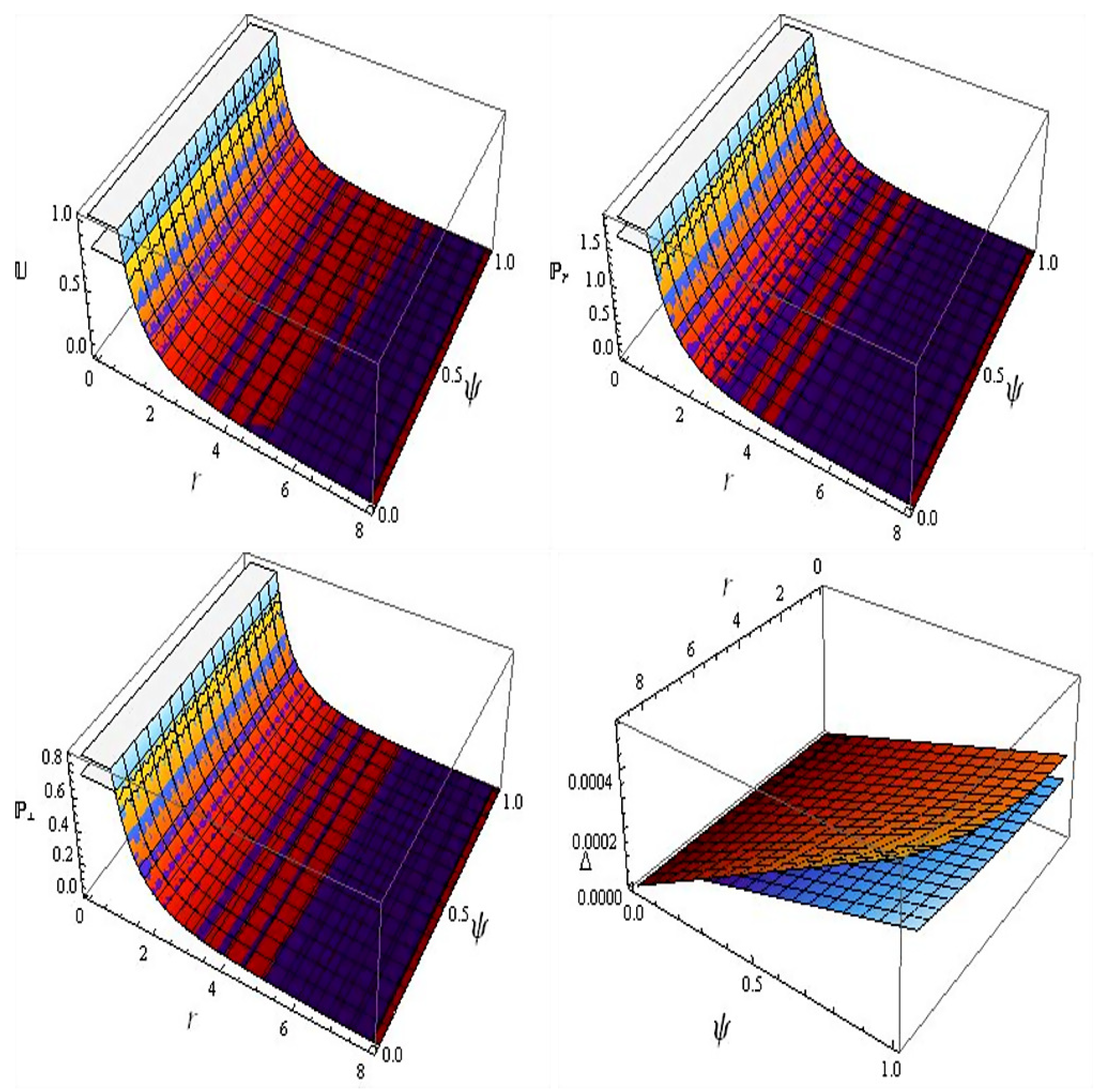
In this section, we analyze the physical aspects, viability and stability of the established solutions corresponding to two stellar entities. For this purpose, the model (8) is chosen, and the values of variables and are fixed to be 1 and −12, respectively. Through the behavior of matter constituents, the feasibility of the astronomical objects is examined. The physical nature of the matter variables (pressure components and energy density) must be positive and maximal closer to the center with diminishing sketch as r rises. The profiles of density and pressure constituents of solution I shown in Figure 1 indicate the maximum behavior at the center and monotonic decrement on reaching the boundary with r. The tangential and radial pressures depict the same trend as that of density and become zero at the star surface. The anisotropy trend in Figure 1 demonstrates that it is zero at the core and maintains this behavior until it reaches the boundary. It is worth noting that anisotropy becomes larger on increasing , and the second star has more anisotropy in comparison to the first one. This ensures the increment in anisotropy in the system as a result of extra source.
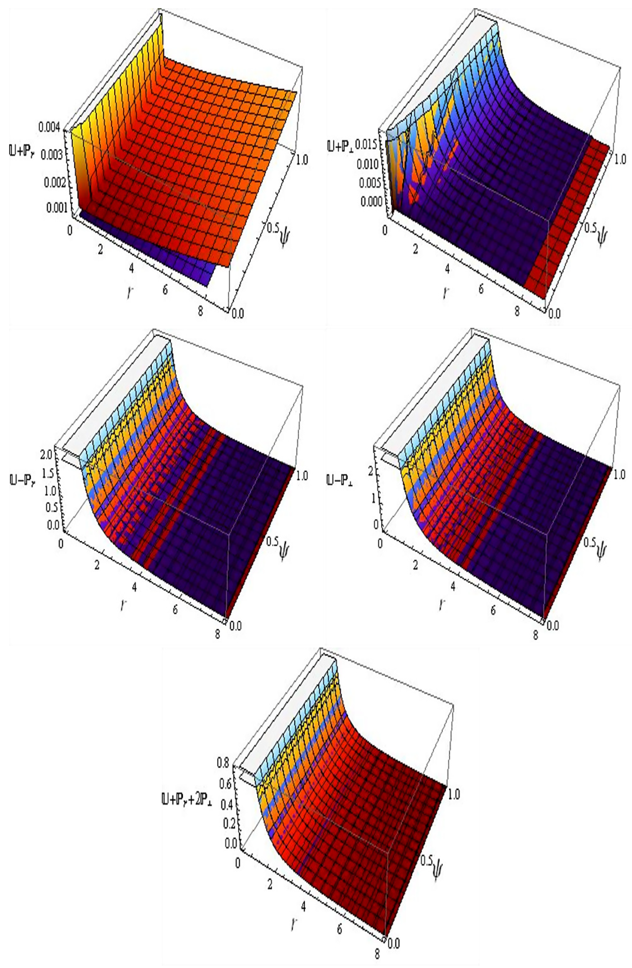
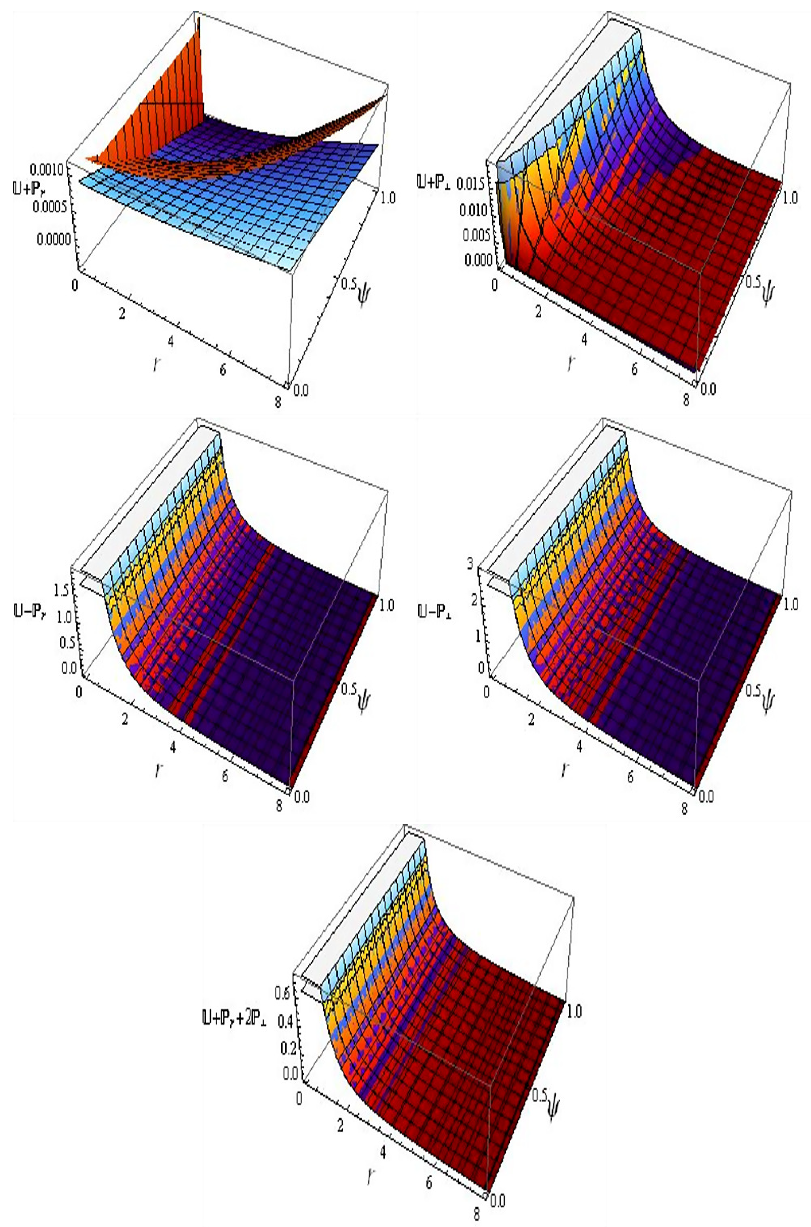
Some mathematical limitations known as energy bounds guarantee the presence of ordinary matter in the inner region of cosmic structures. The fulfillment of these constraints assures the existence of usual source as well as the feasibility of the constructed solutions. These conditions, for the anisotropic matter configuration, are classified as null (NEC), dominant (DEC), weak (WEC) and strong (SEC) as
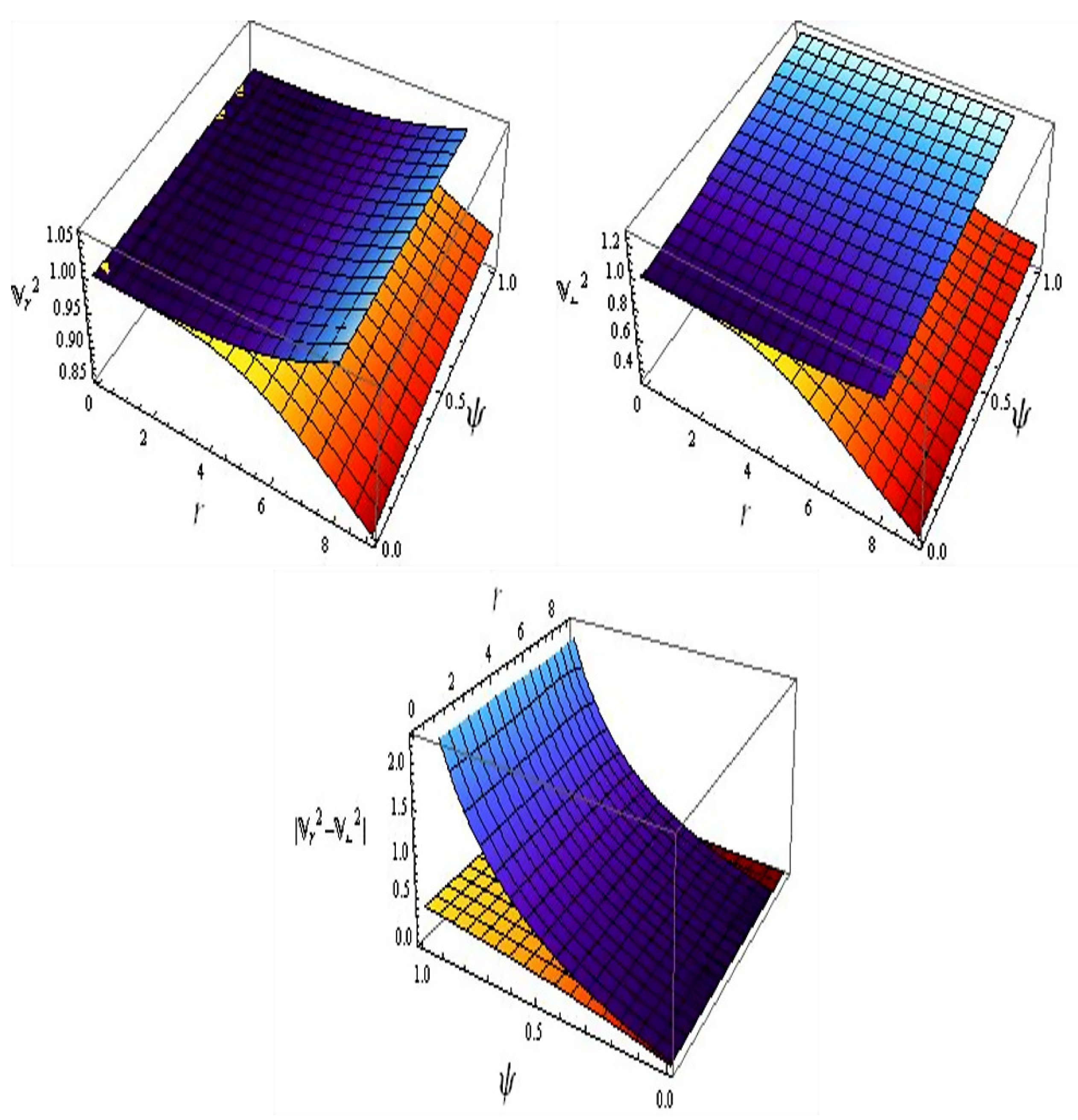
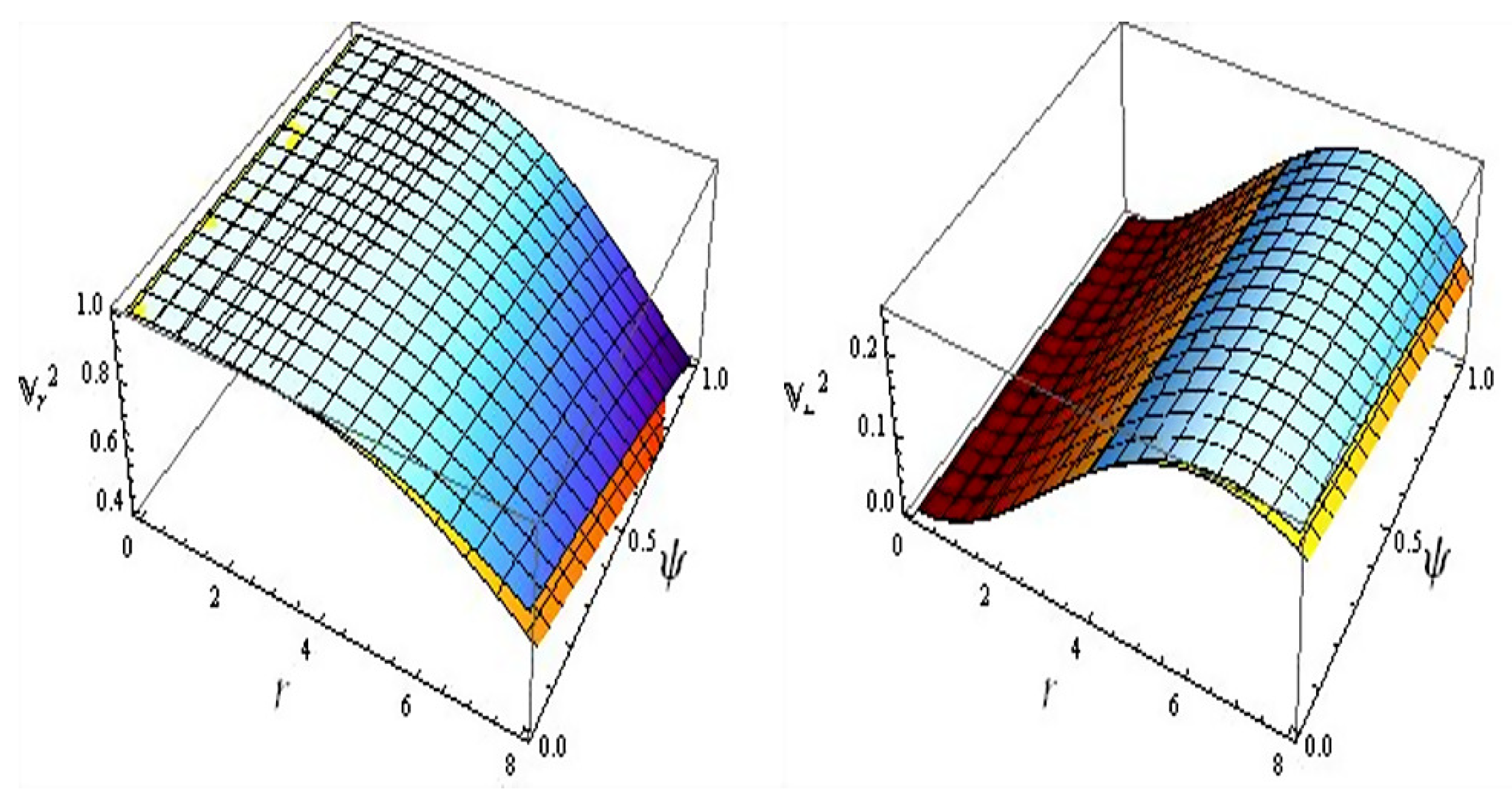
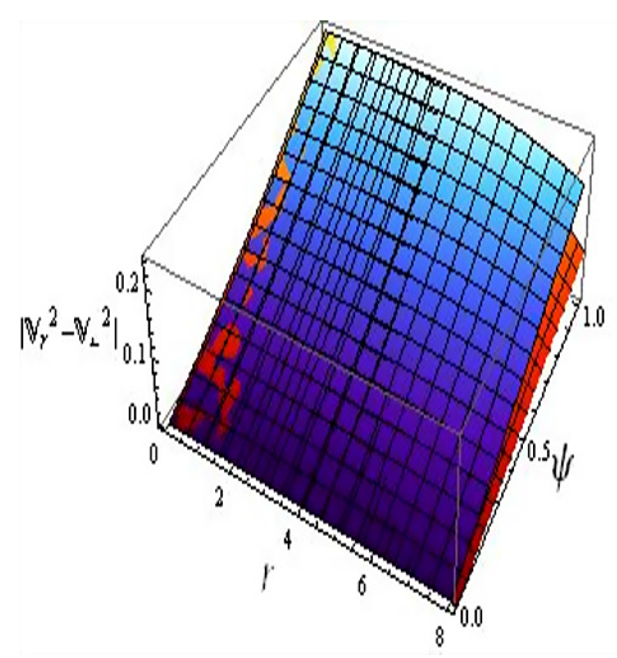
Stability is regarded as an essential feature for analyzing the physical acceptance of stellar structures. We utilize two approaches (Herrera cracking approach and causality condition) to discuss the stable feature of considered astrophysical objects. According to causality condition, the constituents of squared speed of sound must obey [0, 1] or as well as [51], where the radial and tangential ingredients of square speed sound are indicated by and , respectively. Alternatively, we can also say that the speed of sound should be less than the speed of light. The mathematical expressions of speed sound are given as
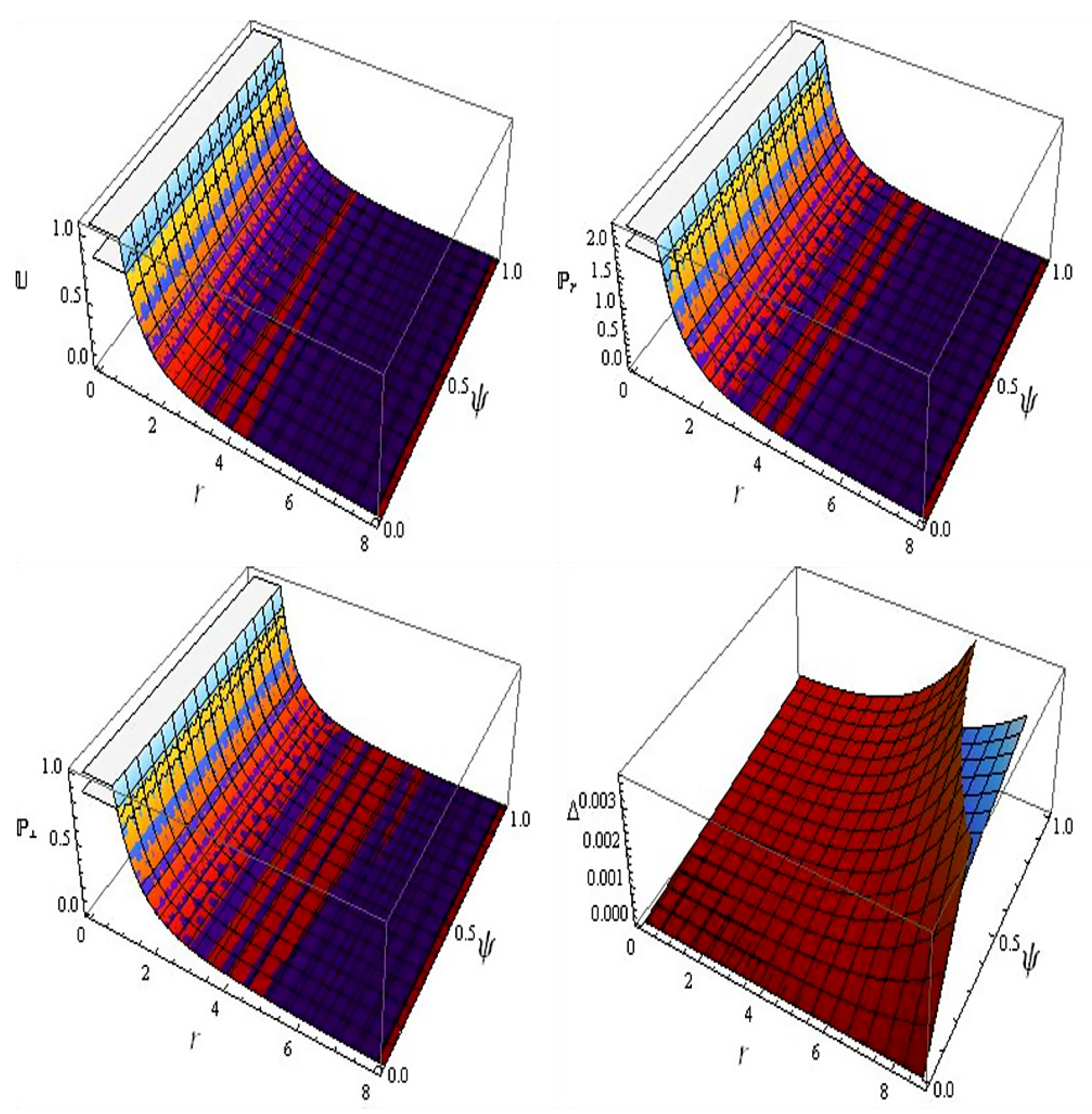
In order to discuss stability, Herrera [52] devised another method called the cracking approach, according to which components of speed sound related to the celestial structures must fulfill the constraint [52]. The stars in Figure 2 illustrate that the first solution is viable as all the necessary requirements for the energy bounds are fulfilled. In Figure 3, one can see that the first solution does not meet the stability criteria for the first candidate. However, for the second model, the similar solution satisfies the stability ranges. To analyze solution II graphically, we make use of the similar values as provided for the first solution. Figure 4 shows that the plots of , and have maximum values at the core and display decreasing behavior as r increases towards the stellar surface. The anisotropy, presented in the last plot of Figure 4, vanishes at the core and sustains this behavior for the whole domain of r. It is also seen that astrophysical objects depict zero anisotropy near the center for every value of decoupling parameter, but it increases near the star surface when the decoupling parameter is increased. Interestingly, similar to solution I, the second star has more anisotropic effects than the first candidate. Figure 5 demonstrates the viability of the second solution since both the stellar structures meet all the energy limitations. The Herrera cracking approach and causality conditions are consistent with the required results for both celestial systems, implying the stability of the solution II (Figure 6).
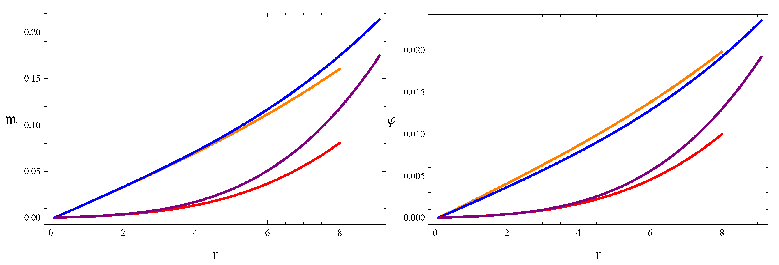
One of the basic entities of a static spherical symmetric geometry is the mass, whose mathematical expression can be defined as
To calculate the mass of the assumed anisotropic stellar models, we numerically solve the above equation together with the initial condition . Compactness () is a necessary substantial property of astrophysical objects, defined as the mass to radius ratio. Buchdahl [53] estimated the maximum bound of the compactness parameter by the matching of inner and outer structures using junction conditions, which was determined to be smaller than . The celestial body produces electromagnetic radiations whose wavelength becomes larger as a result of strong gravitational attraction, hence this change in wavelength is assessed through redshift factor with . Buchdahl revealed that for isotropic matter sources, this value is , while it becomes 5.211 for anisotropic distribution [54]. We assign the decoupling parameter to be for both solutions to analyze the graphical interpretation of mass, compactness and redshift parameters corresponding to two stellar models. The analysis of mass corresponding to solutions I and II is given as
6. Concluding Remarks
This paper deals with static anisotropic spherical solutions using gravitational decoupling method via MGD in the gravity model. The isotropic matter distribution within the static system has been evolved with the addition of an extra sector that introduces anisotropy into the system. Isotropic and anisotropic frameworks are constructed as a result of the deformation of the radial metric component, which splits the system of field equations into two different sets. To resolve the seed source, we have used the Karmarkar condition, which gives rise to particular metric functions, and matching conditions are employed to find the expressions of unknown constants. The second array (24)–(26) has four unknown quantities, so we have closed this system to find the unknowns by applying certain additional constraints on the extra gravitational source. Finally, the physical behavior of the matter determinants as well as viable and stable characteristics of two compact star candidates have been illustrated graphically.
We have discussed physical characteristics of matter variables, anisotropy and energy constraints to ensure that the generated solutions are physically viable. To determine the stable behavior of both solutions, the causality and cracking conditions have been used. We have found that mass, compactness and redshift parameters meet the required limits for both solutions. For both solutions, the star Her X-I is more dense compared to 4U 1820-30. The anisotropic solution I is viable but not stable for the first candidate, while it is both viable as well as stable for the second star. On the other hand, the second anisotropic solution has satisfied all the physical acceptability conditions for both stellar stars. It is important to note that two anisotropic solutions were developed in GR [27], in which only the first solution was viable whereas both solutions were unstable. In the context of gravity, the viable and stable solutions have been found [32,33]. We have also worked on two anisotropic solutions in gravity using Krori–Barua spacetime and found both solutions physically viable as well as the second solution stable [43,44,45]. Here, we have found the results that show more appropriate behavior. Finally, the restrictions in model reduce to GR.
Author Contributions
M.S. suggested the research problem and finalized the manuscript while K.H. did the calculations and prepared the initial draft. All authors have read and agreed to the published version of the manuscript.
Funding
This research received no external funding.
Institutional Review Board Statement
Not applicable.
Data Availability Statement
No new data was generated or used in this paper.
Conflicts of Interest
The authors declare no conflict of interest.
Appendix A
The modified terms are described as
The expressions of GB together with its higher derivative are determined as
References
- Van Albada, T.S.; Sancisi, R. Dark matter in spiral galaxies. Philos. Trans. Royal Soc. A 1986, 320, 447. [Google Scholar]
- Swaters, R.A.; Madore, B.F.; Trewhella, M. High-resolution rotation curves of low surface brightness galaxies. Astrophys. J. 2000, 531, L107. [Google Scholar] [CrossRef] [Green Version]
- Barrow, J.D.; Maartens, R.; Tsagas, C.G. Cosmology with inhomogeneous magnetic fields. Phys. Rep. 2007, 449, 131. [Google Scholar] [CrossRef] [Green Version]
- Neveu, J.; Ruhlmann-Kleider, V.; Astier, P.; Besançon, M.; Guy, J.; Möller, A.; Babichev, E. Constraining the ΛCDM and Galileon models with recent cosmological data. Astron. Astrophys. 2017, 600, A40. [Google Scholar] [CrossRef]
- Deruella, N. On the approach to the cosmological singularity in quadratic theories of gravity: The Kasner regimes. Nuclear. Phys. B 1989, 327, 253. [Google Scholar] [CrossRef] [Green Version]
- Deruella, N.; Farina-Busto, L. Lovelock gravitational field equations in cosmology. Phys. Rev. D 1990, 41, 3696. [Google Scholar] [CrossRef] [Green Version]
- Bhawal, B.; Kar, S. Lorentzian wormholes in Einstein-Gauss-Bonnet theory. Phys. Rev. D 1992, 46, 2464. [Google Scholar] [CrossRef] [PubMed]
- Deruella, N.; Doležel, T. Brane versus shell cosmologies in Einstein and Einstein-Gauss-Bonnet theories. Phys. Rev. D 2000, 10, 103502. [Google Scholar] [CrossRef] [Green Version]
- Nojiri, S.; Odintsov, S.D. Modified Gauss Bonnet theory as gravitational alternative for dark energy. Phys. Lett. B 2005, 631, 1. [Google Scholar] [CrossRef] [Green Version]
- Sharif, M.; Ramzan, A. Anisotropic compact stellar objects in modified Gauss-Bonnet gravity. Phys. Dark Universe 2020, 30, 100737. [Google Scholar] [CrossRef]
- Sharif, M.; Ikram, A. Energy conditions in f(G,T) gravity. Eur. Phys. J. C 2016, 76, 640. [Google Scholar] [CrossRef] [Green Version]
- Sharif, M.; Ikram, A. Stability analysis of some reconstructed cosmological models in f(G,T) gravity. Phys. Dark Universe 2017, 17, 1. [Google Scholar] [CrossRef]
- Sharif, M.; Hassan, K. Complexity factor for static cylindrical objects in f(G,T) gravity. Pramana 2022, 96, 50. [Google Scholar] [CrossRef]
- Sharif, M.; Hassan, K. Complexity of dynamical cylindrical system in f(G,T) gravity. Mod. Phys. Lett. A 2022, 37, 2250027. [Google Scholar] [CrossRef]
- Sharif, M.; Hassan, K. Complexity for dynamical anisotropic sphere in f(G,T) gravity. Chin. J. Phys. 2022, 77, 1479. [Google Scholar] [CrossRef]
- Ruderman, M. Pulsars: Structure and dynamics. Annu. Rev. Astron. Astrophys. 1972, 10, 427. [Google Scholar] [CrossRef]
- Sokolov, A.I. Phase transformations in a superfluid neutron liquid. J. Exp. Theor. Phys. 1980, 49, 1137. [Google Scholar]
- Kippenhahn, R.; Weigert, A.; Weiss, A. Stellar Structure and Evolution; Springer: Berlin/Heidelberg, Germany, 1990. [Google Scholar]
- Herrera, L.; Santos, N.O. Local anisotropy in self-gravitating systems. Phys. Rep. 1997, 286, 53. [Google Scholar] [CrossRef]
- Harko, T.; Mak, M.K. Anisotropic relativistic stellar models. Ann. Phys. 2002, 11, 3. [Google Scholar] [CrossRef]
- Dev, K.; Gleiser, M. Anisotropic stars: Exact solutions. Gen. Relativ. Gravit. 2002, 34, 1793. [Google Scholar] [CrossRef]
- Paul, B.C.; Deb, R. Relativistic solutions of anisotropic compact objects. Astrophys. Space Sci. 2014, 354, 421. [Google Scholar] [CrossRef]
- Arbañil, J.D.V.; Malheiro, M. Radial stability of anisotropic strange quark stars. J. Cosmol. Astropart. Phys. 2016, 11, 012. [Google Scholar] [CrossRef] [Green Version]
- Ovalle, J. Decoupling gravitational sources in general relativity: From perfect to anisotropic fluids. Phys. Rev. D 2017, 95, 104019. [Google Scholar] [CrossRef] [Green Version]
- Ovalle, J.; Casadio, R.; Rocha, R.; Sotomayor, A.; Stuchlík, Z. Black holes by gravitational decoupling. Eur. Phys. J. C 2018, 78, 960. [Google Scholar] [CrossRef] [Green Version]
- Gabbanelli, L.; Rincón, Á.; Rubio, C. Gravitational decoupled anisotropies in compact stars. Eur. Phys. J. C 2018, 78, 370. [Google Scholar] [CrossRef]
- Sharif, M.; Sadiq, S. Gravitational decoupled charged anisotropic spherical solutions. Eur. Phys. J. C 2018, 78, 410. [Google Scholar] [CrossRef] [Green Version]
- Estrada, M.; Tello-Ortiz, F. A new family of analytical anisotropic solutions by gravitational decoupling. Eur. Phys. J. Plus 2018, 133, 453. [Google Scholar] [CrossRef] [Green Version]
- Singh, K.; Maurya, S.K.; Jasim, M.K.; Rahaman, F. Minimally deformed anisotropic model of class one space-time by gravitational decoupling. Eur. Phys. J. C 2019, 79, 851. [Google Scholar] [CrossRef]
- Hensh, S.; Stuchlík, Z. Anisotropic Tolman VII solution by gravitational decoupling. Eur. Phys. J. C 2019, 79, 834. [Google Scholar] [CrossRef] [Green Version]
- Zubair, M.; Azmat, H. Anisotropic Tolman V solution by minimal gravitational decoupling approach. Ann. Phys. 2020, 420, 168248. [Google Scholar] [CrossRef]
- Sharif, M.; Saba, S. Gravitational decoupled charged anisotropic solutions in modified Gauss-Bonnet gravity. Chin. J. Phys. 2019, 59, 481. [Google Scholar] [CrossRef]
- Sharif, M.; Saba, S. Gravitational decoupled Durgapal Fuloria anisotropic solutions in modified Gauss Bonnet gravity. Chin. J. Phys. 2020, 63, 348. [Google Scholar] [CrossRef]
- Sharif, M.; Waseem, A. Effects of charge on gravitational decoupled anisotropic solutions in f(R) gravity. Chin. J. Phys. 2019, 60, 426. [Google Scholar] [CrossRef] [Green Version]
- Sharif, M.; Waseem, A. Anisotropic spherical solutions by gravitational decoupling in f(R) gravity. Ann. Phys. 2019, 405, 14. [Google Scholar] [CrossRef]
- Sharif, M.; Majid, A. Decoupled anisotropic spheres in self-interacting Brans-Dicke gravity. Chin. J. Phys. 2020, 68, 406. [Google Scholar] [CrossRef]
- Sharif, M.; Majid, A. Extended gravitational decoupled solutions in self-interacting Brans Dicke theory. Phys. Dark Universe 2020, 30, 100610. [Google Scholar] [CrossRef]
- Maurya, S.K.; Errehymy, A.; Singh, K.N.; Tello-Ortiz, F.; Daoud, M. Gravitational decoupling minimal geometric deformation model in modified f(R,T) gravity theory. Phys. Dark Universe 2020, 30, 100640. [Google Scholar] [CrossRef]
- Maurya, S.K.; Tello-Ortiz, F.; Ray, S. Decoupling gravitational sources in f(R,T) gravity under class I spacetime. Phys. Dark Universe 2021, 31, 100753. [Google Scholar] [CrossRef]
- Sharif, M.; Naseer, T. Effects of f(R,T,RγυTγυ) gravity on anisotropic charged compact structures. Chin. J. Phys. 2021, 73, 179. [Google Scholar] [CrossRef]
- Naseer, T.; Sharif, M. Study of Decoupled Anisotropic Solutions in f(R,T,RρηTρη) Theory. Universe 2022, 8, 62. [Google Scholar] [CrossRef]
- Sharif, M.; Naseer, T. Isotropization and complexity analysis of decoupled solutions in f(R,T) theory. Eur. Phys. J. Plus 2022, 137, 1304. [Google Scholar] [CrossRef]
- Sharif, M.; Hassan, K. Influence of charge on decoupled anisotropic spheres in f(G,T) gravity. Eur. Phys. J. Plus 2022, 137, 997. [Google Scholar] [CrossRef]
- Sharif, M.; Hassan, K. Anisotropic decoupled spheres in f(G,T) gravity. Int. J. Geom. Methods Mod. Phys. 2022, 19, 2250150. [Google Scholar] [CrossRef]
- Sharif, M.; Hassan, K. Charged Anisotropic Solutions through Decoupling in f(G,T) Gravity. Int. J. Geom. Methods Mod. Phys. 2022. [Google Scholar] [CrossRef]
- Shamir, M.F.; Ahmad, M. Emerging anisotropic compact stars in f(G,T) gravity. Eur. Phys. J. C 2017, 77, 74. [Google Scholar]
- Sharif, M.; Naeem, A. Anisotropic solution for compact objects in f( ) gravity. Int. J. Mod. Phys. A 2020, 35, 2050121. [Google Scholar] [CrossRef]
- Eiesland, J. The group of motions of an Einstein space. Trans. Am. Math. Soc. 1925, 27, 213. [Google Scholar] [CrossRef]
- Maurya, S.K.; Gupta, Y.K.; Dayanandan, B.; Ray, S. A new model for spherically symmetric anisotropic compact star. Eur. Phys. J. C 2016, 76, 266. [Google Scholar] [CrossRef] [Green Version]
- Maurya, S.K.; Gupta, Y.K.; Ray, S.; Deb, D. Generalised model for anisotropic compact stars. Eur. Phys. J. C 2016, 76, 693. [Google Scholar] [CrossRef] [Green Version]
- Abreu, H.; Hernandez, H.; Nunez, L.A. Sound Speeds, Cracking and Stability of Self-Gravitating Anisotropic Compact Objects. Class. Quant. Gravit. 2007, 24, 4631. [Google Scholar] [CrossRef]
- Herrera, L. Cracking of self-gravitating compact objects. Phys. Lett. A 1992, 165, 206. [Google Scholar] [CrossRef]
- Buchdahl, H.A. General relativistic fluid spheres. Phys. Rev. 1959, 116, 1027. [Google Scholar] [CrossRef]
- Ivanov, B.V. Maximum bounds on the surface redshift of anisotropic stars. Phys. Rev. D 2002, 65, 104011. [Google Scholar] [CrossRef] [Green Version]
Figure 1.
Physical analysis of , , and △ versus and r corresponding to two stellar candidates (Solution I).
Figure 1.
Physical analysis of , , and △ versus and r corresponding to two stellar candidates (Solution I).

Figure 2.
Plots of energy constraints versus and r corresponding to two stellar candidates (Solution I).
Figure 2.
Plots of energy constraints versus and r corresponding to two stellar candidates (Solution I).

Figure 3.
Plots of causality condition and Herrera cracking approach versus and r corresponding to two stellar candidates (Solution I).
Figure 3.
Plots of causality condition and Herrera cracking approach versus and r corresponding to two stellar candidates (Solution I).

Figure 4.
Physical analysis of , , and △ versus and r corresponding to two stellar candidates (Solution II).
Figure 4.
Physical analysis of , , and △ versus and r corresponding to two stellar candidates (Solution II).

Figure 5.
Plots of energy constraints versus and r corresponding to two stellar candidates (Solution II).
Figure 5.
Plots of energy constraints versus and r corresponding to two stellar candidates (Solution II).

Figure 6.
Plots of causality condition and Herrera cracking approach versus and r corresponding to two stellar candidates (Solution II).
Figure 6.
Plots of causality condition and Herrera cracking approach versus and r corresponding to two stellar candidates (Solution II).


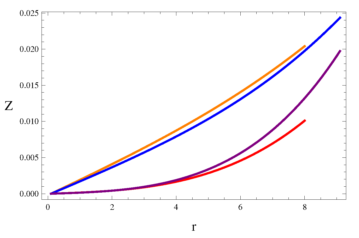
Figure 7.
Plots of mass, compactness and redshift versus r corresponding to (Orange), (Red) (Her X-1) and (Blue) and (Purple) (4U 1820-30) for solution I.
Figure 7.
Plots of mass, compactness and redshift versus r corresponding to (Orange), (Red) (Her X-1) and (Blue) and (Purple) (4U 1820-30) for solution I.


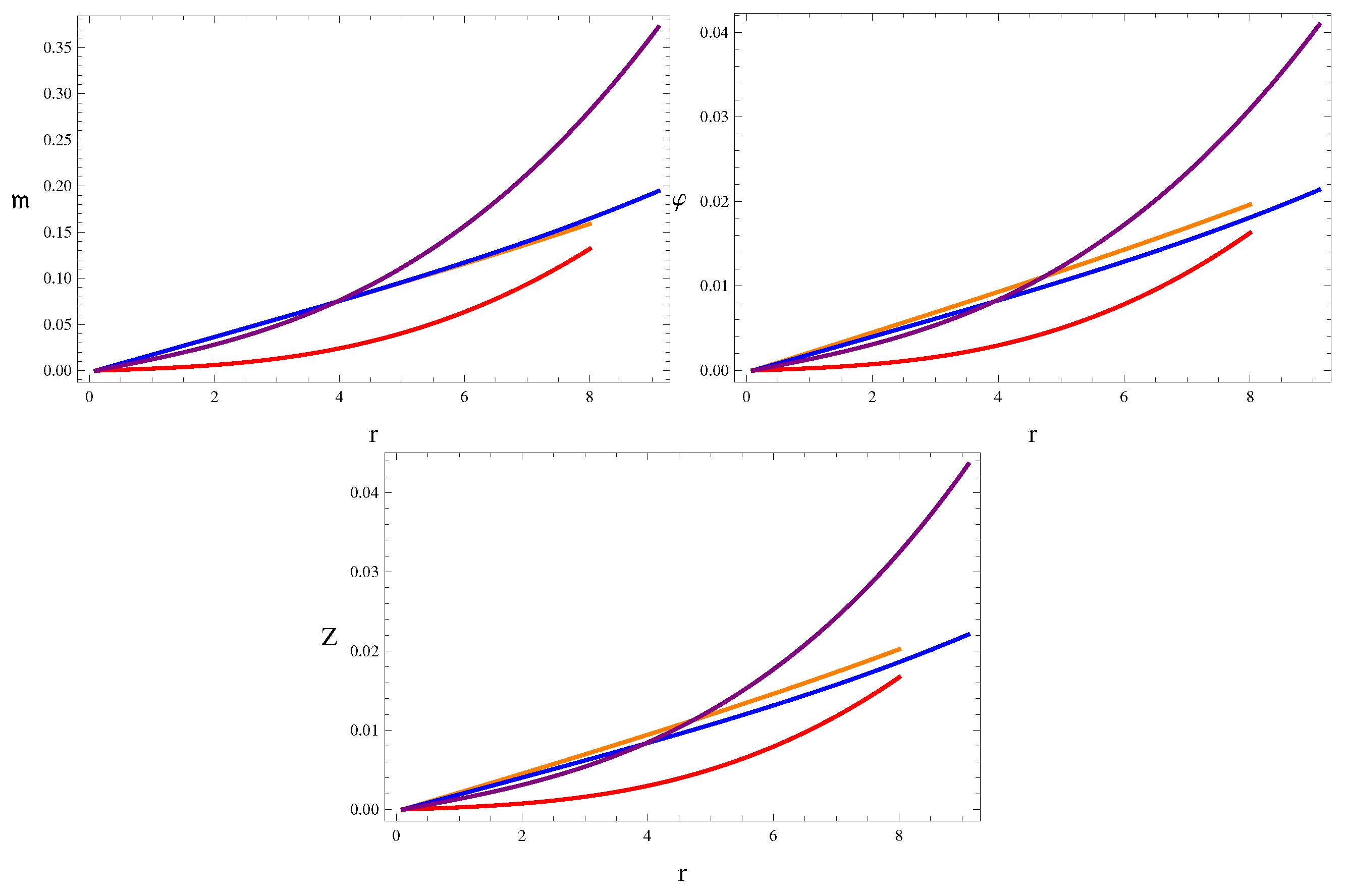
Figure 8.
Behavior of mass, compactness and redshift versus r corresponding to (Orange), (Red) (Her X-1) and (Blue) and (Purple) (4U 1820-30) for solution II.
Figure 8.
Behavior of mass, compactness and redshift versus r corresponding to (Orange), (Red) (Her X-1) and (Blue) and (Purple) (4U 1820-30) for solution II.

Disclaimer/Publisher’s Note: The statements, opinions and data contained in all publications are solely those of the individual author(s) and contributor(s) and not of MDPI and/or the editor(s). MDPI and/or the editor(s) disclaim responsibility for any injury to people or property resulting from any ideas, methods, instructions or products referred to in the content. |
© 2023 by the authors. Licensee MDPI, Basel, Switzerland. This article is an open access article distributed under the terms and conditions of the Creative Commons Attribution (CC BY) license (https://creativecommons.org/licenses/by/4.0/).
Share and Cite
MDPI and ACS Style
Hassan, K.; Sharif, M. Decoupled Anisotropic Solutions Using Karmarkar Condition in f(G, T) Gravity. Universe 2023, 9, 165. https://doi.org/10.3390/universe9040165
AMA Style
Hassan K, Sharif M. Decoupled Anisotropic Solutions Using Karmarkar Condition in f(G, T) Gravity. Universe. 2023; 9(4):165. https://doi.org/10.3390/universe9040165
Chicago/Turabian StyleHassan, Komal, and Muhammad Sharif. 2023. "Decoupled Anisotropic Solutions Using Karmarkar Condition in f(G, T) Gravity" Universe 9, no. 4: 165. https://doi.org/10.3390/universe9040165
Note that from the first issue of 2016, this journal uses article numbers instead of page numbers. See further details here.