Search for Dark Higgs Inflation with Curvature Corrections at LHC Experiments

Abstract

We analyse the dark Higgs inflation model with curvature corrections and explore the possibility to test its predictions by the particle physics experiments at LHC. We show that the dark Higgs inflation model with curvature corrections is strongly favoured by the present cosmological observation. The cosmological predictions of this model, including the quantum corrections of dark Higgs coupling constants and the uncertainty in estimation of the reheating temperature, lead to the dark Higgs mass $m_{\phi }=0.919\pm$ 0.211 GeV and the mixing angle (at 68% CL). We evaluate the FASER and MAPP-1 experiments reach for dark Higgs inflation mass and mixing angle in the 95% CL cosmological confidence region for an integrated luminosity of 3ab${}^{-1}$ at 13 TeV LHC, assuming 100% detection efficiency. We conclude that the dark Higgs inflation model with curvature corrections is a compelling inflation scenario based on particle physics theory favoured by the present cosmological measurements that can leave imprints in the dark Higgs boson searchers at LHC.

1. Introduction

The precise Cosmic Microwave Background (CMB) properties reported by the Planck experiment [1,2,3] and the discovery by LHC of the Higgs boson [4,5] increased the interest in so-called Higgs portal interactions that connect the hidden (dark) sector and the visible sector of the Standard Model (SM), with expected imprints on collider experiments [6]. Scenarios beyond-the-SM (BSM) that introduce a dark sector in addition to the visible SM sector, are required to explain a number of observed phenomena in particle physics, astrophysics and cosmology such as the non-zero neutrino masses and oscillations, Dark Matter (DM), baryon asymmetry of the universe, and cosmological inflation.

It is usual to assume that cosmic inflation is decoupled from the SM at energies lower than the inflationary scale since the slow-roll conditions for inflation generally permit only tiny couplings of the inflation field to other fields. This assumption prevents the direct investigation of the inflation mechanism in particle physics experiments. Consequently, there are few compelling scenarios of inflation based on particle physics theory.

Since the only known fundamental scalar quantum field is the SM Higgs field, the inflation models using the SM Higgs boson as inflation attained great attention over past years. A number of Higgs inflation models, mostly with non-canonical action, have been proposed. They include models with Higgs scalar field non-minimally coupled to gravity [7,8,9], non-minimal derivative coupling to the Einstein tensor [10,11,12,13], scalar-tensor models [14,15], Galileon models [16,17,18,19], and quartic hilltop models [20,21].

The viability of these models is already substantially limited, mostly because they predict tensor-to-scalar ratios larger than the upper bound set by the combined analysis of Planck and BICEP-Keck Array data (hereafter Planck+BK15) that constrain the energy scale of inflation to [2,3]:

$$V_{*}^{1/4}={\left(\frac{3{\pi }^2{A}_s^{*}}{2}{r}_{*}\right)}^{1/4}{M}_{pl}<1.6\times {10}^{16}\mathrm{GeV}(95\%\mathrm{CL}).$$

(1)

Here the quantities with ${(}^{*})$ are evaluated at the pivot scale $k_{*}=0.002$, $r_{*}$ is the ratio of tensor-to-scalar amplitudes, $A_s^{*}$ is the amplitude of the curvature density perturbations and $M_{pl}$ is the reduced Planck mass. This implies an upper bound for the Hubble expansion rate during inflation:

$$H_{*}<2.5\times {10}^{-5}{M}_{pl}(95\%\mathrm{CL}).$$

(2)

The above bound selects the viable Higgs inflation models from the requirement $H_{*}\ll {\Lambda }_c$, where ${\Lambda }_c$ is the unitary bound of each underlying theory, defined as the scale below which the quantum gravitational corrections are sub-leading [22,23,24].

It is worthwhile to mention that the chaotic inflation model with quartic potential is excluded by the data at more than 95% confidence level [25].

Among the models used to lower the predictions for the tensor-to-scalar ratio, the most studied is the Higgs inflation with non-minimal coupling to gravity [7]. At tree level, and for large non-minimal coupling $\xi \sim \mathcal{O}\left({10}^4\right)$, this model gives a small tensor-to-scalar ratio, in agreement with the Planck+BK15 data. However, for such large values of $\xi$, the unitary bound scale, ${\Lambda }_c=M_{pl}/\xi$, could be close or below the energy scale of inflation [22,26].

An interesting framework for Higgs inflation is provided by the scalar-tensor models, including the non-minimal kinetic coupling to the Einstein tensor and to the Gauss–Bonnet invariant. These models can produce inflation simultaneously, satisfying the present inflationary observational constraints and the unitary bound constraints [14,15,27].

Higgs portal interactions via the Renormalisation Group (RG) loop contributions can also lower the predictions of Higgs inflation models for the tensor-to-scalar ratio. The price to pay in these models is the electroweak (EW) vacuum metastability issue. The actual values of Higgs boson and top quark masses imply that the EW vacuum is metastable at energies larger than ${\Lambda }_I\sim {10}^{11}$ GeV, where Higgs quartic coupling turns negative. The actual value of the EW vacuum metastability scale is defined for the top quark mass $m_t=173.15$ GeV and Higgs boson mass $m_h=125.10$ GeV [28] as the value of the Higgs field at which the Higgs quartic coupling, ${\lambda }_h$, becomes negative due to radiative corrections [29,30,31,32].

However, it is found that a small admixture of the Higgs field with an SM scalar singlet with a non-zero vacuum expectation value (vev) can make the EW completely stable due to a tree-level effect on the Higgs quartic coupling, which may be enough to guarantee the stability at large Higgs field values [28,33,34,35].

An appealing scenario in the presence of Higgs portal interactions is given by a SM singlet scalar field with non-zero vev mixed with the SM Higgs boson, often called dark Higgs boson. The dark Higgs mixing with the SM Higgs boson make possible the direct search of the dark Higgs inflation at collider experiments. The mixing guarantees that dark Higgs can be produced in the same channels as the SM Higgs boson if its mass would be the same as that of the dark Higgs boson. Through the same mixing, the dark Higgs boson inherits the SM Higgs boson couplings to SM fermions via the Yukawa interaction term:

$$L\supset \theta \frac{m_f}{v}\phi \overline{f}f,$$

(3)

where $\phi$ is the dark Higgs field, $\theta$ is its mixing angle with the SM Higgs boson and $m_f$ is the fermion mass.

Dark Higgs bosons can be produced at LHC in rare heavy meson decays (such as K and B mesons). They are highly collimated, with characteristic angles $\alpha =M/E$ relative to the parent meson’s direction (M is the meson mass and E is the dark Higgs energy). For $E\sim$ 1 TeV the light dark Higgs decay lengths are of $\mathcal{O}$(${10}^3$ m). Therefore, a significant number of dark Higgs bosons can be detected in faraway detectors of the LHC experiments [6]. Thus, the present and future experimental sensitivity to the light dark Higgs boson decay crucially depends on its production and decay rates and on the detector’s location and acceptance [6,36,37].

The light dark Higgs boson as inflation (rather than the Higgs boson) has been first implemented in Ref. [38], extending the $\nu$MSM model [39,40] to simultaneously explain the cosmological inflation, the DM sterile neutrino masses and the baryon asymmetry of the universe [38,41]. The light dark Higgs inflation properties have been mostly studied in the frame of dark Higgs inflation with non-minimal coupling to gravity [42,43,44,45,46]. A detailed analysis on the possibility to explore this model in the particle physics experiments is presented in Refs. [47,48]. This possibility has also been investigated in the frame of low-scale inflation models, such as the quartic hilltop model [20], predicting a very small value for tensor-to scalar ratio, beyond the sensitivity of the CMB experiments.

In this paper, we analyse the dark Higgs inflation model with non-minimal couplings to gravity and to the Gauss–Bonnet (GB) 4-dimensional invariant and explore the possibility to test its predictions by the particle physics experiments. In this model, the second-order curvature corrections represented by the inflation field coupled to the GB term can increment or suppress (depending on the sign) the tensor-to-scalar ratio [49,50,51,52,53,54]. The possibility to explore this model with the dark Higgs searchers at LHC could provide connections between fundamental theories such as supergravity and string theories, where these couplings are expected to arise, and the Higgs portal interactions.

The paper is organised as follows. In the next section, we discuss the dark Higgs inflation properties. In Section 3, we introduce the dark Higgs inflation model with non-minimal couplings and in Section 4, we analyse the cosmological consistency of its predictions. Section 5 discusses the possibility to test the predictions of the dark Higgs inflation with non-minimal couplings by some representative particle physics experiments at LHC. In Section 6, we draw our conclusions.

Throughout the paper we consider a homogeneous and isotropic flat background described by the Friedmann–Robertson–Walker (FRW) metric:

$$\mathrm{d}{s}^2=g_{\mu ,\nu }\mathrm{d}{x}_{\mu }\mathrm{d}{x}^{\nu }=-\mathrm{d}{t}^2+a^2\left(t\right)d{x}^2,$$

(4)

where a is the cosmological scale factor ($a_0$ = 1 today). Moreover, we use the overdot to denote the time derivative and ${(}^{\prime })$ to denote the derivative with respect to the scalar field.

2. Dark Higgs Model

We consider the scale invariant extension of the SM plus GR with the Lagrangian density given by [55,56,57]:

$$\frac{\mathcal{L}}{\sqrt{-\overline{g}}}=\frac{1}{2{\kappa }^2}({\xi }_{\phi }{\phi }^2+{\xi }_h{h}^2)\mathcal{R}+{\mathcal{L}}_{SM[{\lambda }_h\to 0]}-\frac{1}{2}\partial {\phi }_{\mu }\partial {\phi }_{\nu }-\frac{1}{2}\partial h_{\mu }\partial h_{\nu }+V(h,\phi ),$$

(5)

where ${\mathcal{L}}_{SM[{\lambda }_h\to 0]}$ is the SM Lagrangian without the Higgs potential, $\mathcal{R}$ is the Ricci scalar, ${\kappa }^2=M_{pl}^{-2}$, ${\xi }_h$ and ${\xi }_{\phi }$ are positive coupling constants. We use h to denote the SM Higgs field in the unitary gauge, $h^2=2{\mathcal{H}}^{†}\mathcal{H}$ ( where ${\mathcal{H}}^{†}\mathcal{H}$ is the Higgs doublet ) and $\phi$ to denote the dilaton field, called hereafter the dark Higgs inflation. The scalar potential $V(h,\phi )$ is defined as:

$$V(h,\phi )={\lambda }_h{(\frac{1}{2}{h}^2-\frac{\alpha }{2{\lambda }_h}{\phi }^2)}^2+\beta {\phi }^4,$$

(6)

where $\beta$ and $\alpha$ are positive coupling constants and ${\lambda }_h$ is the SM Higgs field self coupling.

If $\alpha ,\beta \ll {\lambda }_h$, inflation is driven along a flat direction of the scalar potential (6) given by:

$${\mathcal{H}}^{†}\mathcal{H}\simeq \frac{\alpha }{{\lambda }_h}{\phi }^2.$$

(7)

Along this direction the dark Higgs potential is $V\left(\phi \right)=\beta {\varphi }^4/4$ and the coupling constant $\beta$ can be constrained from the requirement to obtain the correct amplitude of curvature density perturbations. This condition leads to $\beta \sim 1.3\times {10}^{-13}$ [58].

The upper bound on the coupling $\alpha$ comes from the requirement that the quantum corrections do not upset the flatness of inflation potential. This constraint leads to $\alpha <3\times {10}^{-7}$ at the tree level [47]. The lower bound on $\alpha$ comes from the requirement to have an efficient conversion of the lepton asymmetry to baryon asymmetry during baryogengesis. This requirement leads to $\alpha >\beta \sim {10}^{-13}$ [38]. A stronger lower bound on $\alpha$ is placed by the estimate of the reheating temperature. For the inflation particles in thermal equilibrium, the reheating temperature is given by [41]:

$$T_r\simeq \frac{\zeta \left(3\right){\alpha }^2}{4{\pi }^2}\sqrt{\frac{90}{g_r}}{\mathrm{M}}_{\mathrm{pl}},$$

(8)

where $g_r=106.75$ is the SM effective number of relativistic degrees of freedom at reheating and $\zeta \left(3\right)=1.202$ is the Reimann zeta function. The requirement that $T_r>150$ GeV ($T\simeq 150$ GeV is the temperature of the EW symmetry breaking), leads to $\alpha >7.3\times {10}^{-8}$.

For a non-thermal distribution of the inflation field the estimate of the reheating temperature is ∼${10}^5{T}_r$, leading to $\alpha >7\times {10}^{-10}$ [59,60].

The couplings in the Lagrangian (5) are energy scale-dependent and may be changed when quantum corrections are take into account. For this reason it is useful to write $V(h,\phi )$ in terms of couplings ${\lambda }_i$:

$$V(h,\phi )=\frac{1}{4}{\lambda }_h{h}^4-\frac{1}{4}{\lambda }_{h\phi }{h}^2{\phi }^2+\frac{1}{4}{\lambda }_{\phi }{\phi }^4$$

(9)

where ${\lambda }_{h\phi }=2\alpha$ and ${\lambda }_{\phi }\simeq \beta$. In this paper, we take the RG beta-functions of the relevant couplings following Refs. [31,42,44,45].

2.1. Light Dark Higgs Mass and Mixing Angle

Under the metric transformation:

$$\begin{array}{c}\hfill g_{\mu \nu }={\Omega }^2{\overline{g}}_{\mu \nu },\Omega =({\xi }_{\phi }{\phi }^2+{\xi }_h{h}^2)/M_{pl}^2,\end{array}$$

(10)

the potential (6) in the Einstein frame reads as:

$$\begin{array}{c}\hfill U(h,\phi )=\frac{M_{pl}^4}{{\Omega }^{2}V(h,\phi )}=\frac{M_{pl}^4}{{({\xi }_{\phi }{\phi }^2+{\xi }_h{h}^2)}^2}\times \left({\lambda }_h{(\frac{1}{2}{h}^2-\frac{\alpha }{2{\lambda }_h}{\phi }^2)}^2+\beta {\phi }^4\right).\end{array}$$

(11)

One should note that we have neglected the contribution of ${\mathcal{R}}^2$ term in the Lagrangian (5) as the field $\phi$ is equivalent to a new scalaron field that is degenerated with the non-minimal couplings ${\xi }_h$ and ${\xi }_{\phi }$ under the metric redefinition [61,62,63].

The minimisation condition of the potential:

$$\frac{\mathrm{d}U(h,\phi )}{\mathrm{d}h}{|}_{h=\mathit{v},\phi =\mathit{w}}=0,$$

(12)

where $\mathit{v}$ and $\mathit{w}$ are the corresponding vacuum expectation values, sets the hierarchy parameter $\vartheta$ and the dark Higgs inflation mixing angle $\theta$ to:

$$\begin{array}{c}\hfill {\vartheta }^2\equiv \frac{{\mathit{v}}^2}{{\mathit{w}}^2}=\frac{\alpha }{{\lambda }_h}+\frac{4\beta {\xi }_h}{{\lambda }_h{\xi }_{\phi }+\alpha {\xi }_h},tan2\theta \simeq \frac{\mathit{v}}{\mathit{w}}.\end{array}$$

(13)

We emphasise that the SM Higgs boson mass is given by $m_h=\sqrt{2{\lambda }_h}\mathit{v}$, where $\mathit{v}\equiv {\left(\sqrt{2}{G}_F\right)}^{1/2}=246.22$ GeV is fixed by the Fermi coupling constant $G_F$, and the experimentally measured Higgs boson mass is $m_h=125.10\pm 0.14$ GeV [28].

The corresponding mass-matrix:

$${\mathcal{M}}^2=2\times \left(\begin{array}{cc}{\lambda }_h{\mathit{v}}^2& \alpha \mathit{v}\mathit{w}\\ \alpha \mathit{v}\mathit{w}& \beta {\mathit{w}}^2\end{array}\right),$$

can be diagonalised by the orthogonal transformation $O^T{\mathcal{M}}^{2}O=\mathrm{diag}(m_{\tilde{h}}^2,m_{\tilde{\phi }}^2)$ [64]:

$$O=\left(\begin{array}{cc}cos\theta & sin\theta \\ -sin\theta & cos\theta \end{array}\right).$$

The mass squared eigenvalues are than given by [65]:

$$m_{\tilde{h},\tilde{\phi }}^2={\lambda }_h{\mathit{v}}^2+{\lambda }_{\phi }{\mathit{w}}^2\frac{{\lambda }_{\phi }{\mathit{w}}^2-{\lambda }_h{\mathit{v}}^2}{cos2\theta }.$$

(14)

Since we are interested in the case with

$m_{\phi }\ll m_h$ and $\alpha ,\beta \ll {\lambda }_h$, we find: $\theta \simeq \mathit{v}/\mathit{w}$, $m_{\tilde{h}}^2=2{\lambda }_h{\mathit{v}}^{\mathit{2}}$ and $m_{\tilde{\phi }}^2=2{\lambda }_{\tilde{\phi }}{\mathit{w}}^{\mathit{2}}$.

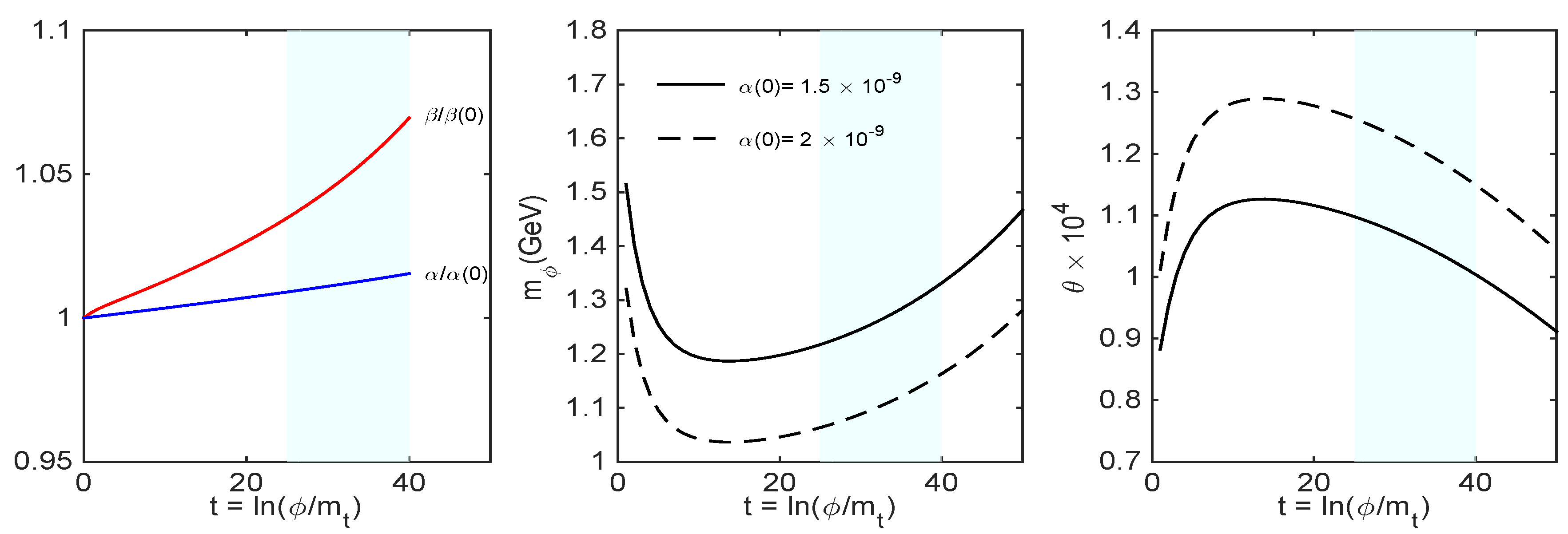
Figure 1 presents the RG evolution with the energy scale of $\beta$ and $\alpha$ coupling constants, the dark Higgs mass $m_{\phi }$ and the mixing angle $\theta$, showing the stability of these parameters relative to the radiative corrections in the inflationary regime.

2.2. Reheating and Horizon Crossing

Reheating proceeds by the energy transfer from the dark Higgs inflation field to the SM Higgs particles through a regime of parametric resonance [59,60]. At early stages, the entire energy is in the inflation zero-mode and all other modes are absent. The inflation zero-mode oscillations excite the non-zero modes of the inflation and of the SM Higgs particles. This parametric resonance regime ends before a significant part of the inflation zero-mode energy is depleted [41]. The reason is the SM Higgs re-scattering process that becomes important quite early because of the large SM Higgs self-coupling ($\lambda \sim 0.1$).

After the end of the parametric resonance regime, the fluctuations of the inflation field continue to grow exponentially while the energy transferred to the SM Higgs field is negligible. The SM Higgs re-scattering processes bring the inflation particles in the thermal equilibrium and the reheating proceeds through the decay of the dark Higgs inflation into the SM degrees of freedom.

If reheating occurs after the electroweak symmetry breaking (EWSB) the dark Higgs field evolves as cold dark matter from ESWB onwards, and the universe becomes matter-dominated until reheating occurs [66]. To prevent the restoration of the EW symmetry after reheating, a late inflation decay is required such as the reheating temperature $T_r\le m_W\simeq$ 80 GeV. These low reheating temperatures require non-thermal baryogenesis such as the Affleck–Dine mechanism [67,68]. We note that the condition required for nucleosynthesis is $T_r>$ 10 MeV. This scenario requires a dark Higgs mass of few GeV that may be probed by the future LHC experiments.

If instead reheating occurs before EWSB, the inflation evolves like dark radiation from reheating until EWSB and the post-inflationary universe becomes radiation-dominated. In this scenario, the temperature at which EWSB occurs is $\sim 7\times {10}^5$ GeV [66]. Consequently, the EW symmetry is restored by the thermal effects and the dark Higgs remains massless, behaving as dark radiation.

The inflationary observables are evaluated at the epoch of the Hubble crossing scale $k_{*}$ (pivot scale) quantified by the number of e-folds $\mathcal{N}$ before the end of the inflation. Therefore, the uncertainties in the determination of $\mathcal{N}$ translates into theoretical uncertainties in determination of the inflationary observables [42,69]. Assuming that the ratio of the today entropy per co-moving volume to that after reheating is negligible, the main error $\Delta \mathcal{N}$ in the determination of $\mathcal{N}$ is given by the uncertainty in the determination of the reheating temperature $T_r$. The number of e-foldings at Hubble crossing scale $k_{*}$ is related to $T_r$ through:

$$\mathcal{N}=\log \left[{\left(\frac{{\rho }_r}{{\rho }_e}\right)}^{1/4}{\left(\frac{g_0{T}_0^3}{g_r{T}_r^3}\right)}^{1/3}\left(\frac{k_{*}}{a_0{H}_0}\right)\right],$$

(15)

where ${\rho }_r$ and ${\rho }_e$ refer to the densities at reheating and at the end of inflation, $T_0$ is the present photon temperature, $H_{*}$ is the Hubble parameter at $k_{*}$, $g_r=106.75$ and $g_0=43/11$ are the effective numbers of relativistic degrees of freedom at reheating and at present time. From (8) and (15) we obtain $\Delta \mathcal{N}\simeq 3$, corresponding to the uncertainty in determination of $T_r$ for the thermal distribution of the inflation field. This uncertainty is four times higher in the case of a non-thermal distribution.

3. Dark Higgs Inflation with Curvature Corrections

In this section, we consider that inflation is driven by the dark Higgs field potential $V\left(\varphi \right)=\beta {\phi }^4/4$ along the flat direction defined in (13).

We briefly discuss the Dark Higgs inflation model assuming non-minimal coupling of the dark Higgs field to the Ricci scalar and to the GB invariant. To simplify formulas, in this section we choose the Planck units.

We consider that the dark Higgs model is described by the following action:

$$S=\int {\mathrm{d}}^{4}x\sqrt{-g}\left[F\left(\phi \right)\mathcal{R}-\frac{g^{\mu \nu }}{2}{\partial }_{\mu }\phi {\partial }_{\nu }\phi -V\left(\phi \right)-\frac{1}{2}g\left(\phi \right){\mathcal{G}}_{GB}\right],$$

(16)

where $V\left(\phi \right)$ is the dark Higgs potential, $\mathcal{R}$ is the Ricci scalar, $F\left(\phi \right)$ and $g\left(\phi \right)$ are coupling functions and ${\mathcal{G}}_{GB}$ is the Gauss–Bonnet invariant: ${\mathcal{G}}_{GB}={\mathcal{R}}^2-4{\mathcal{R}}_{\mu \nu }{\mathcal{R}}^{\mu \nu }+{\mathcal{R}}_{\mu \nu \delta \rho }{\mathcal{R}}^{\mu \nu \delta \rho }$.

For a homogeneous and isotropic flat background described by the FRW metric (4) the expression for the Ricci scalar $\mathcal{R}$ and the Gauss-Bonnet invariant ${\mathcal{G}}_{GB}$ are given by [70]:

$$\begin{array}{c}\hfill \mathcal{R}=6(H^2+\dot{H}),{\mathcal{G}}_{GB}=24H^2(H^2+\dot{H}),\end{array}$$

(17)

where $H=\dot{a}/a$ is the Hubble parameter, and $a\left(t\right)$ is the cosmological scale factor.

The variation of action (16) leads to the following evolution evolutions [53,71,72]:

$$\begin{array}{ccc}\hfill 6H^2\left(F-4H{g}^{{}^{\prime }}\dot{\phi }\right)& =& {\dot{\phi }}^2+2V-6H{F}^{{}^{\prime }}\dot{\phi },\hfill \end{array}$$

(18)

$$\begin{array}{ccc}\hfill 2\dot{H}\left(F-4H{g}^{{}^{\prime }}\dot{\phi }\right)& =& 4H^2\left(\ddot{g}-{\dot{\phi }}^2-H{g}^{{}^{\prime }}\dot{\phi }\right)-\ddot{F}+H{F}^{{}^{\prime }}\dot{\phi },\hfill \end{array}$$

(19)

$$\begin{array}{ccc}\hfill \ddot{\phi }+3H\dot{\phi }& =& 3\left(\dot{H}+2H^2\right)F^{{}^{\prime }}-V^{{}^{\prime }},-12g^{{}^{\prime }}{H}^2\left(\dot{H}+H^2\right).\hfill \end{array}$$

(20)

In the slow-roll approximation [71]:

$$\begin{array}{c}\hfill {\dot{\phi }}^2\ll V,|\ddot{\phi }|\ll 3H|\dot{\phi }|,4|\dot{g}|H\ll F,|\ddot{g}|\ll H|\dot{g}|,|\ddot{F}|\ll H|\dot{F}|\ll H^{2}F,\end{array}$$

(21)

Equations (18)–(20) read as:

$$\begin{array}{ccc}\hfill 3F{H}^2& \simeq & V,\hfill \end{array}$$

(22)

$$\begin{array}{ccc}\hfill 2F\dot{H}& \simeq & -{\dot{\phi }}^2-4H^3{g}^{{}^{\prime }}\dot{\phi }+H{F}^{{}^{\prime }}\dot{\phi },\hfill \end{array}$$

(23)

$$\begin{array}{ccc}\hfill \dot{\phi }& \simeq & -\frac{V^{{}^{\prime }}+12g^{{}^{\prime }}{H}^4-6H^2{F}^{{}^{\prime }}}{3H}.\hfill \end{array}$$

(24)

The slow-roll approximation (21) requires $|{ϵ}_0|,|{ϵ}_1|,...|{\Delta }_1|\ll 1$, where the slow-roll parameters are defined as:

$$\begin{array}{c}\hfill {ϵ}_0=-\frac{\dot{H}}{H^2},{ϵ}_1=\frac{{\dot{ϵ}}_0}{H{ϵ}_0},{\zeta }_0=\frac{\dot{F}}{HF},{\zeta }_1=\frac{{\dot{\zeta }}_0}{H{\zeta }_0},{\Delta }_0=\frac{4H{\dot{F}}_1}{F},{\Delta }_1=\frac{{\dot{\Delta }}_0}{H{\Delta }_0}.\end{array}$$

(25)

The number of e-folds before the end of inflation is then given by:

$$\mathcal{N}={\int }_{{\phi }_I}^{{\phi }_E}\frac{H}{\dot{\phi }}\mathrm{d}\phi ={\int }_{{\phi }_I}^{{\phi }_E}\frac{3H^2}{6H^2{F}^{{}^{\prime }}-12g^{{}^{\prime }}{H}^4-V^{{}^{\prime }}},$$

(26)

where ${\phi }_I$ and ${\phi }_E$ are the values of the field at the beginning and at the end of inflation. The value of ${\varphi }_E$ is obtained from the requirement ${ϵ}_0=1$, while (26) allows the determination of ${\varphi }_I$ at $\mathcal{N}$e-folds before the end of inflation.

In terms of slow-roll parameters, the amplitude of scalar density perturbations $A_s$, the scalar spectral index $n_s$ and the tensor-to-scalar ratio r expressed at the Hubble crossing scale $k_{*}$ are given by [71]:

$$\begin{array}{ccc}\hfill A_s& \simeq & \frac{H^2}{4{\pi }^{2}F|2{ϵ}_0+{\zeta }_0-{\Delta }_0|},\hfill \end{array}$$

(27)

$$\begin{array}{ccc}\hfill n_s& =& 1-2{ϵ}_0-\frac{2{ϵ}_0({\zeta }_0+{ϵ}_1)+{\zeta }_0({\zeta }_0+{\zeta }_1)-{\Delta }_0({\zeta }_0-{\Delta }_1)}{2{ϵ}_0+{\zeta }_0-{\Delta }_0},\hfill \end{array}$$

(28)

$$\begin{array}{ccc}\hfill r& =& 8\frac{2{ϵ}_0+{\zeta }_0-{\Delta }_0}{1-{\Delta }_0}.\hfill \end{array}$$

(29)

Hereafter, we will take the coupling functions $F\left(\phi \right)$ and $g\left(\phi \right)$ of the form:

$$\begin{array}{c}\hfill F\left(\phi \right)=1+{\xi }_{\phi }{\phi }^2,g(\phi )=\eta {\phi }^{-4}\end{array}$$

(30)

where ${\xi }_{\phi }$ is the scale-dependent coupling of the inflation field with gravity while $\eta$ is a positive constant during inflation with the dimension $\left[\eta \right]=M_{pl}^4$.

It is convenient to write $\beta \eta =\tilde{\alpha }{M}_{pl}^4$, where $\tilde{\alpha }$ is a dimensionless parameter that defines the behaviour of the inflation field once the number of e-folds has been fixed.

4. Cosmological Constraints

4.1. Parameterisation and Methods

The dark Higgs baseline cosmological model is described by the following parameters:

$$\mathbf{P}=\left\{{\Omega }_b{h}^2,{\Omega }_c{h}^2,{\theta }_s,\tau ,\mathcal{N},\beta ,\alpha ,{\xi }_{\phi },\tilde{\alpha }\right\},$$

(31)

where: ${\Omega }_b{h}^2$ is the present baryon energy density, ${\Omega }_c{h}^2$ is the present CDM energy density, ${\theta }_s$ is the ratio of sound horizon to angular diameter distance at decoupling, $\tau$ is the optical depth at reionization, $\mathcal{N}$ is the number of e-folds introduced to account for the uncertainty in the determination of the reheating temperature, $\beta$ is the dark Higgs quartic coupling, $\alpha$ is the SM Higgs - dark Higgs coupling, ${\xi }_h$ and ${\xi }_{\phi }$ are the SM Higgs and dark Higgs couplings to gravity and $\tilde{\alpha }$ parametrise the inflation coupling to the GB invariant.

We compute the dependence on the scaling variable $t=\ln (\varphi /m_t)$ ($m_t=171.15$ GeV is the top quark mass) of the running of various coupling constants by integrating the corresponding beta-functions:

$$\begin{array}{c}\hfill {\beta }_{{\lambda }^i}=\frac{\partial {\lambda }^i}{\partial t},{\lambda }^i=\{g,g^{{}^{\prime }},g_s,y_t,\beta ,\alpha ,{\xi }_h,{\xi }_{\phi }\},\end{array}$$

(32)

where $g,g^{{}^{\prime }},g_s$ are the gauge couplings, $y_t$ is the Yukawa coupling (for the relevant beta functions see Appendix A from [44] and references therein).

At $t=0$, the SM Higgs self coupling ${\lambda }_h\left(0\right)=0.129$ and the top Yukawa coupling is the $y_t\left(0\right)=0.976$ are fixed by the SM Higgs and top quark pol masses [31].

For the gauge couplings at $t=0$ we take $g^{{}^{\prime }}\left(0\right)=0.364$, $g\left(0\right)=0.64$ and $g_s\left(0\right)=1.161$ [73]. The priors for $\beta$, $\alpha$, and ${\xi }_{\phi }$ at $t=0$ are given in

Table 1. Priors and constraints on the parameters of dark Higgs inflation model with curvature corrections adopted in the analysis. All priors are uniform in the listed intervals. We assume a flat universe.

Parameter	Prior
${\Omega }_b{h}^2$	[0.005, 0.1]
${\Omega }_c{h}^2$	[0.001, 0.5 ]
$100{\theta }_s$	[0.5, 10]
$\tau$	[0.01, 0.9]
$\mathcal{N}$	[54, 64]
$\alpha \times {10}^7$	[0.007, 3]
$\beta \times {10}^{13}$	[1, 5]
$\tilde{\alpha }$	[0, 3]
${\xi }_{\phi }$	[0, 1]
$H_0({\mathrm{km}\mathrm{s}}^{-1} {\mathrm{Mpc}}^{-1})$	[20, 100]

(see below).

It is important to note that ${\xi }_h\left(t\right)$ is generated via the RG runnings (32).

We modify the standard Boltzmann code CAMB v.1.1.2 (accessed on 31 May 2020) http://camb.info [74] to evolve the coupled dark Higgs field Equations (22)–(24) with respect to the conformal time for wave numbers in the range $5\times {10}^{-6}$–5 Mpc${}^{-1}$, compute the slow-roll parameters and evaluate the amplitude of scalar density perturbations $A_s$, the scalar spectral index $n_s$ and the tensor-to-scalar ratio r at the Hubble crossing scale $k_{*}=0.002$Mpc${}^{-1}$.

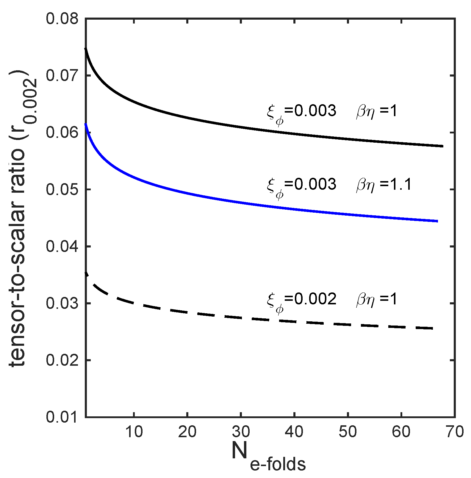
Figure 2 presents the evolution with the number of e-folds $\mathcal{N}$ of the tensor-to-scalar ratio $r_{0.002}$ evaluated at the Hubble crossing scale $k_{*}=0.002$Mpc${}^{-1}$, obtained for different values of the coupling constants ${\xi }_{\phi }$ and $\tilde{\alpha }$.

The extraction of parameters from the cosmological dataset is based on Monte-Carlo Markov Chains (MCMC) technique. We modify the publicly available version of the package CosmoMC v. 3.2.1 http://cosmologist.info/cosmomc/ (accessed on 31 May 2020) [75] to sample from the space of dark Higgs inflation model parameters and generate estimates of their posterior mean and confidence intervals.

We made some test runs to optimise the parameters prior intervals and sampling. The final run is based on 120 independent channels, reaching the convergence criterion $(R-1)\simeq 0.01$. The $(R-1)$ criterion is defined as the ratio between the variance of the means and the mean of variances for the second half of chains [75].

We assume a flat universe and uniform priors for all parameters adopted in the analysis in the intervals listed in Table 1. The Hubble expansion rate $H_0$ is a derived parameter in our analysis. We constrained $H_0$ values to reject the extreme models.

For the cosmological analysis we use the CMB temperature (TT), polarization (EE,TE) and lensing angular power spectra from Planck 2018 release [1] and the likelihood codes corresponding to different multipole intervals http://pla.esac.esa.int/pla/cosmology, accessed on 31 May 2020. The Planck data currently provide the best characterisation of the primordial density perturbations [2], constraining the cosmological parameters at the sub-percent level [1].

We use the following combinations of TT, TE, EE and lensing Planck likelihoods [2]:

(i) Planck TT + lowE: the combination of high-l TT likelihood at multipoles l ≥ 30, the Commander likelihood for low-l temperature-only and the SimAll low-l EE likelihood in the range 2 < l < 29; (ii) Planck TE and Planck EE: the combination of TE and EE likelihoods at l ≥ 30; (iii) Planck TT,TE,EE+lowE: the combination of Commander likelihood using TT, TE, and EE spectra at $\mathit{l}$ ≥ 30, the low-l temperature, and the low- SimAll EE likelihood; (iv) Planck TT, TE, EE + lowP: the combination of the likelihoods using TT, TE, and EE spectra at l > 30; (v) Planck high-l and Planck low-l polarization: the Plik likelihood; (vi) Planck CMB lensing: the CMB lensing likelihood [76] for lensing multipoles 8 < l < 400.

We also consider the measurement of the CMB B-mode polarization power spectrum by the BICEP2/Keck Array collaboration [3]. The BK15 likelihood B-mode polarization only leads to an upper limit of tensor-to-scalar ratio amplitudes $r<$ 0.07 (95% CL) [3].

We will refer to the combination of these datasets as Planck TT, TE, EE + lowE + lensing + BK15.

4.2. Analysis

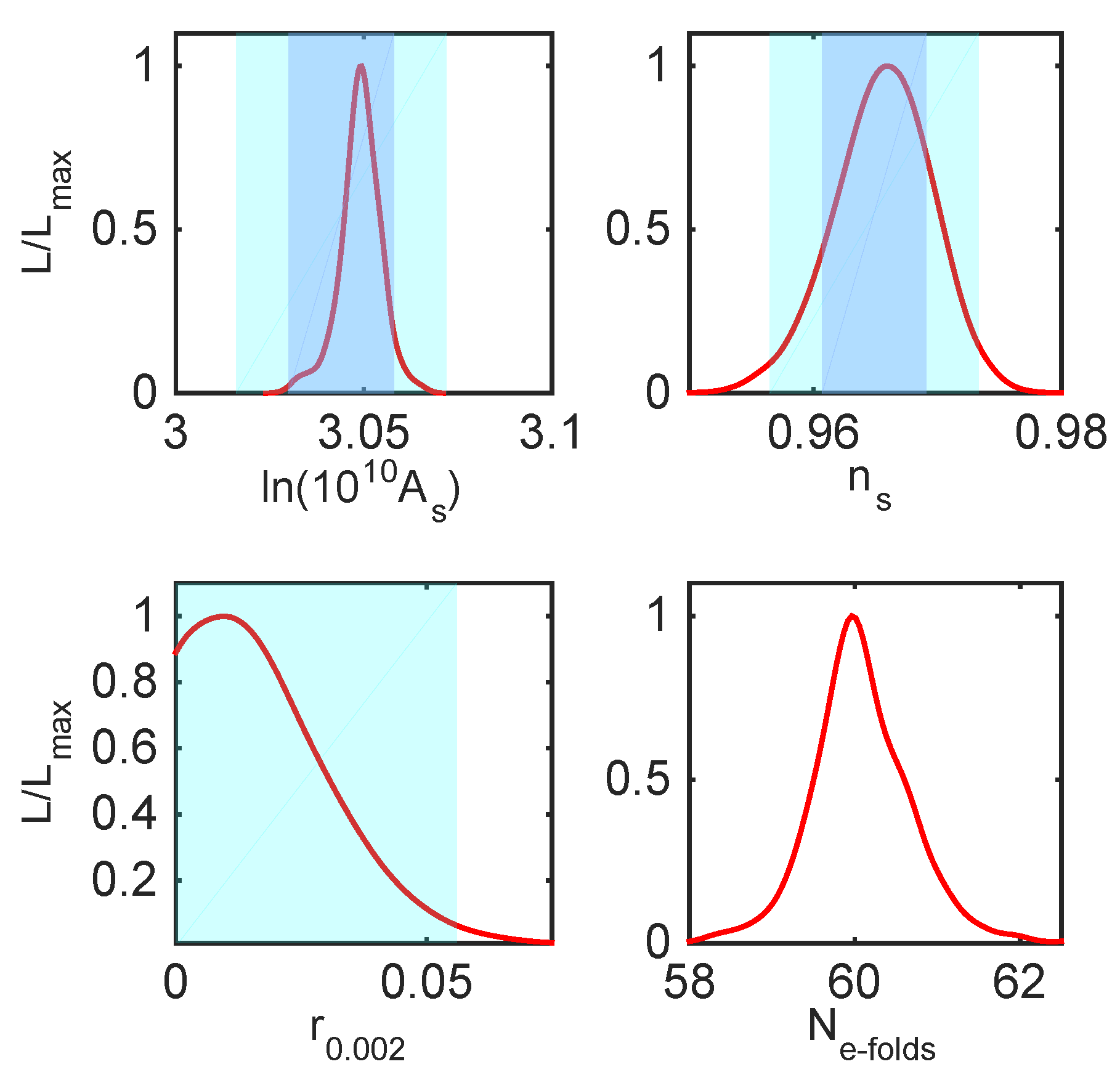
Figure 3 presents the marginalised likelihood probability distributions of the inflationary parameters, $A_s$, $n_s$, r and $\mathcal{N}$ from the fit of the dark Higgs inflation model with curvature corrections with the Planck TT,TE,EE+lowE+lensing+BK15 dataset. These predictions are computed at pivot scale $k_{*}$ = 0.002 Mpc${}^{-1}$ and include the uncertainty in the number of e-folds. For comparison, we also show the corresponding 65% and 95% limits from the fit of $\Lambda$CDM model with the same dataset [2]. The mean values and the errors for all parameters are presented in

Table 2. The mean values and the absolute errors of the main parameters obtained from the fit of the dark Higgs inflation model with curvature corrections with Planck TT, TE, EE + lowE + lensing + BK15 dataset. The errors are quoted at 68% CL. The upper limits are quoted at 95% CL. The first group of parameters are the base cosmological parameters sampled in the Monte-Carlo Markov Chains analysis with uniform priors.The others are derived parameters.

Parameter
${\Omega }_b{h}^2$	0.0223 ± 0.0002
${\Omega }_c{h}^2$	0.1194 ± 0.0011
${\theta }_s$	1.0410 ± 0.0004
$\tau$	0.050 ± 0.009
$r_{0.002}$	<0.059
$\mathcal{N}$	59.4 ± 1.210
${10}^{13}\times \beta$	0.892 ± 0.051
${10}^9\times \alpha$	1.021 ±0.219
$\tilde{\alpha }=\beta \eta /M_{pl}^4$	0.879±1.215
${\xi }_{\phi }$	<0.0023
$H_0\left({\mathrm{km}\mathrm{s}}^{-1}{\mathrm{Mpc}}^{-1}\right)$	67.729 ± 0.641
$\ln \left({10}^{10}{A}_s\right)$	3.050 ± 0.008
$n_s$	0.967 ± 0.0044
$m_{\phi }$ (GeV)	0.919 ± 0.211
${10}^4\times \theta$	1.291 ± 0.045

.

We find that the dark Higgs inflation model with curvature corrections is strongly favoured by the Planck+BK15 data [2].

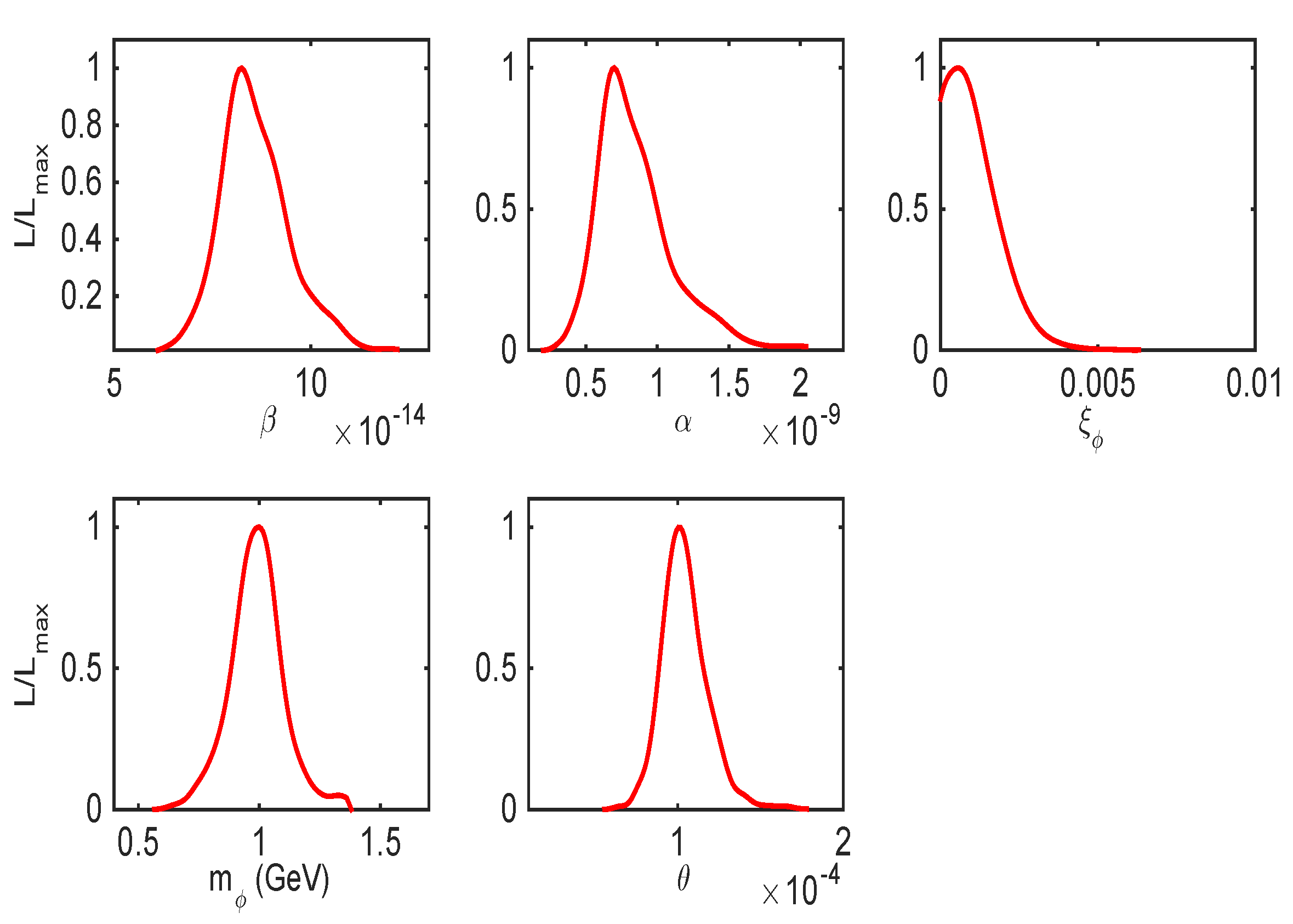
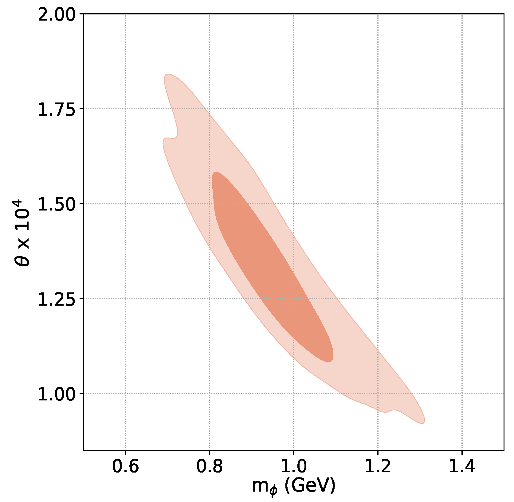
Figure 4 presents the likelihood probability distributions of the dark Higgs parameters $\beta$, $\alpha$, ${\xi }_{\phi }$,$m_{\phi }$ and $\theta$ obtained from the fit of the dark Higgs inflation model with the Planck TT,TE,EE+lowE+lensing+BK15 dataset. In Figure 5, we show the marginalised joint 68% and 95% CL regions obtained for $m_{\phi }$ and $\theta$.

The mean values and the errors of these parameters are given in Table 2.

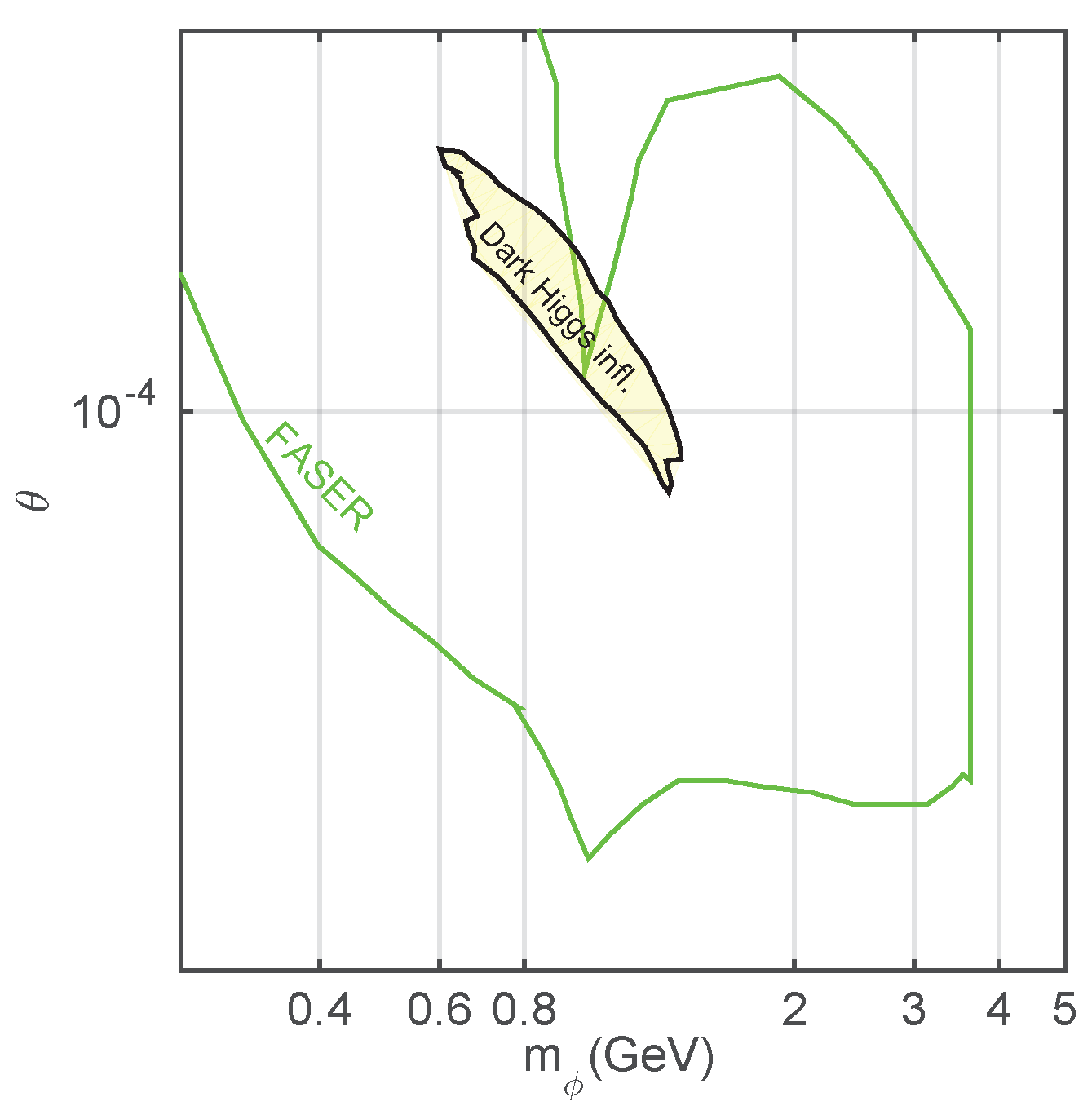
The bounds on dark Higgs mass and mixing angle (at 95% CL):

$$\begin{array}{c}\hfill 0.4\mathrm{GeV}<m_{\phi }<1.4\mathrm{GeV},4.5\times {10}^{-5}<\theta <1.8\times {10}^{-4},\end{array}$$

(33)

are in the range of expected sensitivity of Forward Physics Facility (FPF) experiments at LHC proposed in the framework of beyond-the-SM physics [6].

5. Search for Dark Higgs Inflation at LHC Experiments

5.1. Dark Higgs Inflation Decay

The dark Higgs mixing with the SM Higgs boson makes the direct search of the dark Higgs inflation at collider experiments possible.

The dark Higgs decay widths are suppressed by ${\theta }^2$ relative to those of the SM Higgs boson if it would have the some mass as the dark Higgs.

For $m_{\phi }<2m_{\pi }$ the inflation mostly decays in $e^{+}{e}^{-}$, ${\mu }^{+}{\mu }^{-}$ and ${\tau }^{+}{\tau }^{-}$ with decay width given by:

$$\begin{array}{c}\hfill \Gamma (\phi \to \overline{l}l)=G_F\frac{m_l^2{m}_{\phi }}{4\sqrt{2}\pi }{\beta }_l^3{\theta }^2(l=e,\mu ,\tau ),\end{array}$$

(34)

where $G_F$ is the Fermi constant and ${\beta }_l=\sqrt{1-m_l^2/m_{\phi }^2}$ is the lepton velocity.

For inflation masses in the range $2m_{\pi }<m_{\phi }<2.5$ GeV the dominant decay modes are to ${\pi }^{+}{\pi }^{-}$, $k^{+}{k}^{-}$ and other hadrons.

The dark Higgs hadronic decay modes suffer from theoretical uncertainties since the chiral expansion breaks down above $2m_{\pi }$ while the perturbative QCD calculations are reliable for masses of few GeV [77,78].

For the inflation mass range (33), we adopt the numerical results from [78] that use the dispersive analysis for $2m_{\pi }<m_{\phi }<1.3$ GeV [79], the perturbative spectator model for $m_{\phi }>$ 2 GeV [80,81] and interpolate between these two for 1.3 GeV$<m_{\phi }<$ 2 GeV.

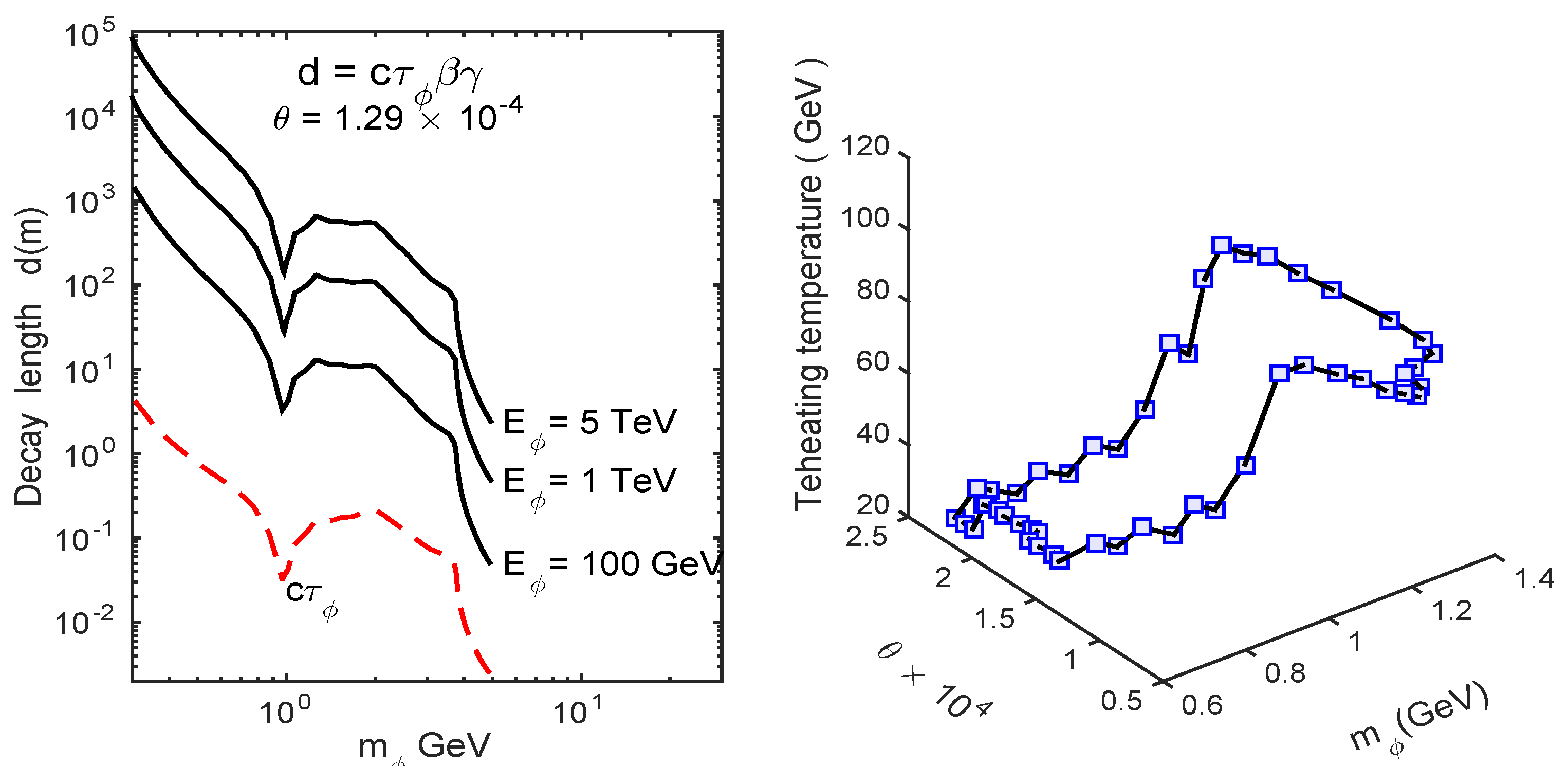
The left panel from Figure 6 presents the dependence on $E_{\phi }$ of the dark Higgs decay length:

$$\begin{array}{c}\hfill d=c{\tau }_{\phi }\gamma \beta \end{array}$$

(35)

where ${\tau }_{\phi }=1/\Gamma (\varphi \to ll,hh)$ is the dark Higgs lifetime, $\Gamma (\phi \to ll,hh)$ is the decay width scaled with ${\theta }^2$, $\gamma =E_{\phi }/m_{\phi }$ and $\beta =\sqrt{1-1/{\gamma }^2}$.

The decay length scales as $d\sim E_{\phi }$ for large $E_{\phi }$. For $E_{\phi }\sim \mathcal{O}\left({10}^3\right)$ GeV the decay lengths are d$\sim \mathcal{O}\left(1\right)$ km and therefore a significant number of dark Higgs inflations can decay within the detector volume.

5.2. Dark Higgs Reheating Temperature and Energy Density

The reheating temperature is directly related to the total decay width ${\Gamma }_{\phi }$ of the inflation with mass $m_{\phi }$ and mixing angle $\theta$ through [27,46]:

$$T_r\simeq {\left(\frac{90}{{\pi }^2{g}^{*}}\right)}^{1/4}\theta {\left({\Gamma }_{\phi }\times M_{pl}\right)}^{1/2}.$$

(36)

The right panel from Figure 6 presents the estimates of reheating temperature in dark Higgs parameter space (33). For best fit values ($m_{\phi },\theta$) at 68% CL we obtain $T_r=$62.83 GeV, indicating that in this model reheating occurs after EWSB.

The present dark Higgs energy density can be estimated as [66]:

$${\Omega }_{\phi ,0}=\frac{m_{\phi }^2}{3H_0^2{M}_{pl}^2}{\phi }_r^2\frac{g_0}{g^{*}}{\left(\frac{T_0}{T_r}\right)}^3,$$

(37)

where the ${\phi }_r$ is the dark Higgs field amplitude at $T_r$.

In our model, the reheating occurs after EWSB, therefore, the dark Higgs field behaves like radiation before EWSB such that $\phi \sim a^{-1}$, and like CDM onwards, such that $\phi \sim a^{-3/2}$. The dark Higgs field at reheating is then obtained as:

$$\begin{array}{c}\hfill {\phi }_r\left(a_r\right)={\phi }_E{\left(\frac{a_{EW}}{a_E}\right)}^{-1}{\left(\frac{a_r}{a_{EW}}\right)}^{-3/2},\end{array}$$

(38)

where ${\phi }_E$ is the dark Higgs field at the end of inflation and $a_E$, $a_{EW}$ and $a_r$ are the scale factors corresponding to the end of inflation, EWSB and reheating.

Assuming that EWSB occurs at $T_{EW}=m_W\simeq 80$ GeV, such that EW symmetry after reheating is not restored, taking $T_r=$ 62.83 GeV and ${\phi }_E$ = 1.46 M${}_{pl}$, we obtain ${\Omega }_{\phi ,0}\simeq$ 0.004 for or best fit values $(m_{\phi },\theta )$ at 68% CL, representing around 1.5% from total CDM energy density today (${\Omega }_{c,0}\simeq$ 0.26).

5.3. Dark Higgs Decay Inside Detector

To determine the number of dark Higgs inflations that decay inside the detector volume, we must specify the size, shape, and location of the detector relative to the LHC collider interaction point (IP).

We consider two representative experiments, FASER (the ForwArd Search ExpeRiment) [82,83] and MAPP (the MoEDAL Apparatus for Penetrating Particles) [84]:

• The FASER detector has a cylindrical shape centred on the LHC beam collision axis at $L_{max}$ = 480 m from IP, has an available length $\Delta$ = 15 m and the radius R = 2 m.
• The MAPP detector is a parallelepiped at approximately $5^{\circ }$ from the beam collision axis at $L_{max}=100$ m from IP with an available length $\Delta =3$ m and the parallelepiped height $H=1$ m.

The probability of the dark Higgs boson to decay inside the detector volume is given by:

$${\mathcal{P}}^{det}(E_{\phi },{\theta }_{\alpha })=\left(e^{-L_{min}/d}-e^{-L_{max}/d}\right)\Theta (R,tan\left({\theta }_{\alpha }\right)L_{max})$$

(39)

where $L_{min}=L_{max}-\Delta$, $E_{\phi }$ is the dark Higgs energy, d is its decay length, ${\theta }_{\alpha }$ is the angular acceptance of the detector, $tan\left({\theta }_{\alpha }\right)=R/L_{max}$, and $\Theta$ is the Heaviside step function. For MAPP, we take $R=H{\pi }^{-1/2}$ in (39) to conserve the effective acceptance area.

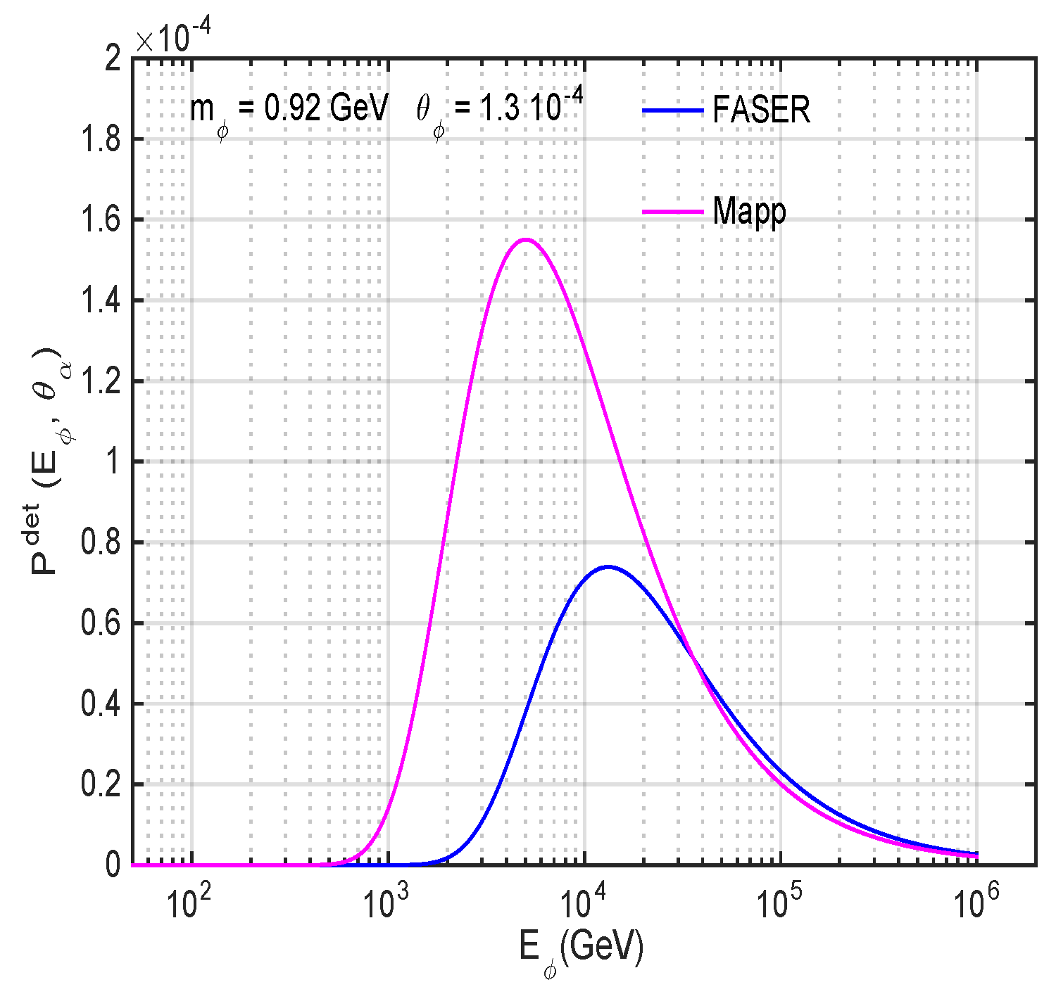
In Figure 7, we present the dependence on $E_{\phi }$ of the normalised detection probability corresponding to the above experimental configurations obtained for the cosmological best fit solution for $m_{\phi }$ and $\theta$. The figure shows that the experimental configurations are sensitive to complementary ranges of the dark Higgs energy.

5.4. Dark Higgs Production

The dark Higgs bosons can be produced in K and B meson decays as well as in lighter meson decays like $\eta$ and $\pi$. The branching ratios are proportional with ${\theta }^2$ and are largest for processes involving heavyer flavours as B mesons. For $m_{\varphi }>m_K$ ($m_K=0.494$ GeV), the most efficient mechanism of dark Higgs production is the decay of B mesons produced in $pp$ collisions dominated by the process $b\to s\phi$, with $\phi$ radiated from the top-quark [37]. The branching fraction for both $B^0$ and $B^{\pm }$ mesons is given by [47,85,86]:

$$Br(B\to X_s\phi )\simeq 0.3\frac{|V_{ts}{V}_{tb}^{*}{|}^2}{|V_{cb}{|}^2}{\left(\frac{m_t}{m_W}\right)}^4{\left(1-\frac{m_{\phi }^2}{m_B^2}\right)}^2{\theta }^2,$$

(40)

where $X_s$ denotes any strange hadronic state, $m_B$, $m_t$ and $m_W$ are the corresponding masses for B meson, top-quark and W-boson, and $V_{ts}$, $V_{tb}$ and $V_{cb}$ are the Cabibbo–Kobayashi–Maskawa (CKM) matrix elements [28].

The dark Higgs production cross section at LHC energies can be estimated as [47]:

$$\begin{array}{c}\hfill {\sigma }_{\phi }={\sigma }_B\times Br(B\to X_s\varphi ),\end{array}$$

(41)

where ${\sigma }_B$ is the B meson production cross-section for $pp\to B\chi$ interactions.

We assume an integrated luminosity of 3 a$b^{-1}$ in $pp$ collisions at the centre-of-mass energy $\sqrt{s}$ = 13 TeV, implying a total number of inelastic $pp$ scattering events $N_{inel}\simeq 1.1\times {10}^{16}$, the $pp$ multiplicity $M_{pp}\simeq$ 66 and the $pp$ inelastic cross-section ${\sigma }_{pp}$(13 TeV) ≃ 75 mb [28].

We also take the B meson total production cross-section ${\sigma }_B$(13 TeV) = 86.5 µb [87].

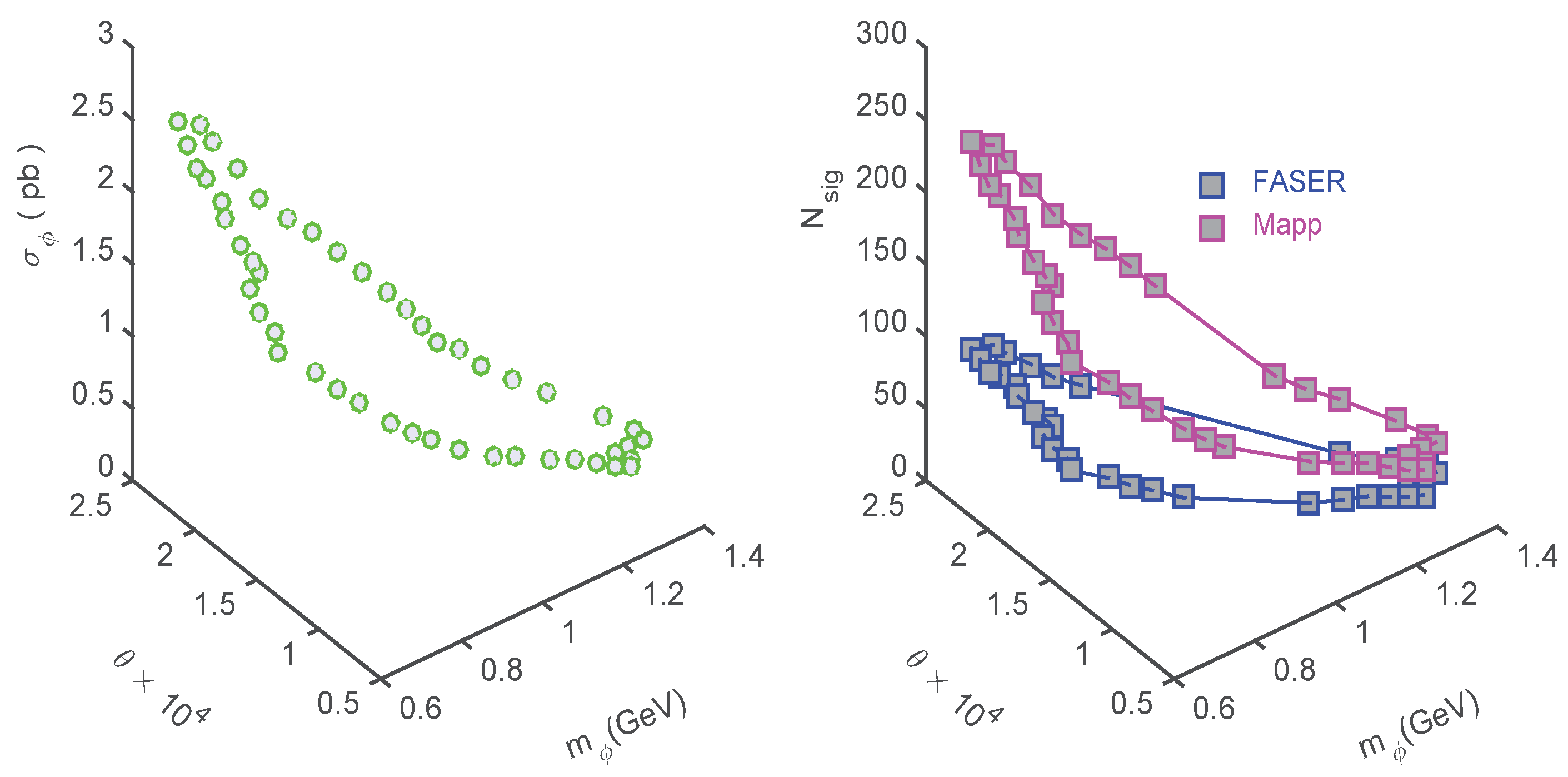
Left panel from Figure 8 presents the dark Higgs cross-section ${\sigma }_{\phi }$ in the cosmological confidence region (33). We obtain $Br(B\to X_s\phi )\simeq 2.2\times {10}^{-8}$ and ${\sigma }_{\phi }\simeq$ 0.92 pb for our best fit solution for ($m_{\phi },\theta$) at 68% CL.

One should note that the SM Higgs total cross-section at $\sqrt{s}$ = 13 TeV is $57\pm 5.9$ pb [28].

5.5. LHC Experiments Reach for Dark Higgs Inflation with Curvature Couplings

The total number of dark Higgs bosons that decay inside the detector are then given by:

$$N_{sig}(m_{\phi },\theta )=N_{inel}\frac{{\sigma }_{\phi }}{{\sigma }_{inel}}Br(\varphi \to KK)Br(\phi \to \pi \pi )\int {\mathcal{P}}^{det}(E_{\phi },{\theta }_{\alpha })\mathrm{d}{\theta }_{\alpha }\mathrm{d}{E}_{\phi }.$$

(42)

The right panel from Figure 8 shows the predicted number of dark Higgs signal events $N_{sig}$ in the cosmological confidence region (33) obtained for FASER and MAPP experimental configurations assuming 100% detection efficiency.

We take the dark Higgs energy in the range 100 GeV $<E_{\varphi }<10{}^6$ GeV, imposed by the requirement that the dark Higgs inflation propagate to the detector locations.

In Figure 9, we compare the number of signal events in the dark Higgs parameter space (33) with the FASER expected number of signal events for an integrated luminosity of 3ab${}^{-1}$ at 13 TeV LHC assuming 100% detection efficiency [37].

6. Conclusions

In this paper, we analyse the dark Higgs inflation model with curvature corrections given by the non-minimal coupling of the inflation field to the Ricci scalar and the Gauss–Bonnet (GB) invariant and explore the possibility to test its predictions by the particle physics experiments at LHC.

The dark Higgs model considered ensures that the scale invariance is explicitly broken on the classical level in the inflation sector, leading to non-zero vev for the dark Higgs inflation after reheating.

We show that the dark Higgs inflation model with curvature corrections is strongly favoured by Planck + BK15 data [2].

The cosmological predictions for dark Higgs inflation mass $m_{\phi }$ and mixing angle $\theta$, including the RG quantum corrections and the uncertainty in estimation of the reheating temperature (33) are in the range of expected sensitivity of Forward Physics Facility (FPF) experiments at LHC. We also show that in this scenario, reheating takes place after EWSB, making the dark Higgs inflation a valuable CDM candidate.

We evaluate the FASER and MAPP experiments reach for dark Higgs inflation parameters $m_{\varphi }$ and $\theta$ assuming 100% detection efficiency, for an integrated luminosity of 3ab${}^{-1}$ at the the centre-of-mass energy $\sqrt{s}=$13 TeV.

We conclude that the dark Higgs inflation model with curvature corrections is a compelling inflation scenario based on particle physics theory favoured by the present cosmological measurements, leaving imprints in the dark Higgs boson searchers at LHC.

References

- Aghanim, N.; Akrami, Y.; Ashdown, M.; Aumont, J.; Baccigalupi, C.; Ballardini, M.; Banday, A.J.; Barreiro, R.B.; Bartolo, N.; Basak, S.; et al. Planck 2018 results VI. Cosmological parameters. Astron. Astrophys. 2020, 641, A10. [Google Scholar]
- Akrami, Y.; Arroja, F.; Ashdown, M.; Aumont, J.; Baccigalupi, C.; Ballardini, M.; Banday, A.J.; Barreiro, R.B.; Bartolo, N.; Basak, S.; et al. Planck 2018 results. X. Constraints on inflation. Astron. Astrophys. 2020, 641, A6. [Google Scholar]
- Ade, P.A.R.; Ahmed, Z.; Aikin, R.W.; Alexander, K.D.; Barkats, D.; Benton, S.J.; Bischoff, C.A.; Bock, J.J.; Bowens-Rubin, R.; Brevik, J.A.; et al. BICEP2/Keck Array X: Constraints on Primordial Gravitational Waves using Planck, WMAP, and New BICEP2/Keck Observations through the 2015 Season. Phys. Rev. Lett. 2018, 121, 221301. [Google Scholar] [CrossRef] [Green Version]
- ATLAS Collaboration; Aad, G.; Abajyan, T.; Abbott, B.; Abdallah, J.; Khalek, S.A.; Abdelalim, A.A.; Abdinov, O.; Aben, R.; Abi, B.; et al. Observation of a new particle in the search for the Standard Model Higgs boson with the ATLAS detector at the LHC. Phys. Lett. 2012, 761, 1–29. [Google Scholar]
- Chatrchyan, S.; Khachatryan, V.; Sirunyan, A.M.; Tumasyan, A.; Adam, W.; Aguilo, E.; Bergauer, T.; Dragicevic, M.; Erö, J.; Fabjan, C.; et al. Observation of a new boson at a mass of 125 GeV with the CMS experiment at the LHC. Phys. Lett. 2012, 716, 30. [Google Scholar] [CrossRef]
- Beacham, J.; Burrage, C.; Curtin, D.; De Roeck, A.; Evans, J.; Feng, J.L.; Gatto, C.; Gninenko, S.; Hartin, A.; Irastorza, I.; et al. Physics Beyond Colliders at CERN Beyond the Standard Model Working Group Report. J. Phys. G 2020, 47, 010501. [Google Scholar] [CrossRef]
- Bezrukov, F.L.; Shaposhnikov, M. The Standard Model Higgs boson as the inflaton. Phys. Lett. 2008, 659, 703. [Google Scholar] [CrossRef] [Green Version]
- Futamase, T.; Maeda, K.-I. Chaotic Inflationary Scenario in Models Having Nonminimal Coupling with Curvature. Phys. Rev. 1989, 39, 399. [Google Scholar]
- Fakir, R.; Unruh, W.G. Improvement on cosmological chaotic inflation through nonminimal coupling. Phys. Rev. 1990, 41, 1783. [Google Scholar] [CrossRef]
- Germani, C.; Kehagias, A. New Model of inflation with Nonminimal Derivative Coupling of Standard Model Higgs Boson to Gravity. Phys. Rev. Lett. 2010, 105, 011302. [Google Scholar] [CrossRef] [Green Version]
- Granda, L.N. Inflation driven by scalar field with non-minimal kinetic coupling with Higgs and quadratic potentials. JCAP 2011, 04, 016. [Google Scholar] [CrossRef] [Green Version]
- Granda, L.N.; Jimenez, D.F.; Cardona, W. Higss inflation with non-minimal derivative coupling to gravity. Astropart. Phys. 2020, 121, 102459. [Google Scholar] [CrossRef]
- Tsujikawa, S. Observational tests of inflation with a field derivative coupling to gravity. Phys. Rev. 2012, 85, 083518. [Google Scholar] [CrossRef] [Green Version]
- Granda, L.N.; Jimenez, D.F. Higgs Inflation with linear and quadratic curvature corrections. arXiv 2019, arXiv:1910.11289. [Google Scholar]
- Granda, L.N.; Jimenez, D.F. Slow-Roll Inflation in Scalar-Tensor Models. JCAP 2019, 9, 7. [Google Scholar] [CrossRef] [Green Version]
- Kamada, K.; Kobayashi, T.; Yamaguchi, M.; Yokoyama, J. Higgs G-inflation. Phys. Rev. 2011, 83, 083515. [Google Scholar]
- Ohashi, J.; Tsujikawa, S. Potential-driven Galileon inflation. JCAP 2012, 1210, 035. [Google Scholar] [CrossRef] [Green Version]
- Kobayashi, T.; Yamaguchi, M.; Yokoyama, J. Inflation Driven by the Galileon Field. Phys. Rev. Lett. 2010, 105, 231302. [Google Scholar] [CrossRef] [Green Version]
- Kobayashi, T.; Yamaguchi, M.; Yokoyama, J. Generalized G-inflation: Inflation with the most general second-order field equations. Prog. Theor. Phys. 2011, 126, 511. [Google Scholar] [CrossRef]
- Bramante, J.; Cook, J.; Delgado, A.; Martin, A. Low scale inflation at high energy colliders and meson factories. Phys. Rev. 2016, 94, 115012. [Google Scholar] [CrossRef] [Green Version]
- German, G. Quartic hilltop inflation revisited. JCAP 2021, 2, 34. [Google Scholar] [CrossRef]
- Burgess, C.P.; Lee, H.M.; Trott, M. Power-counting and the Validity of the Classical Approximation During Inflation. JHEP 2009, 9, 103. [Google Scholar] [CrossRef] [Green Version]
- Bezrukov, F.; Magnin, A.; Shaposhnikov, M.; Sibiryakov, S. Higgs inflation: Consistency and generalisations. JHEP 2011, 11, 16. [Google Scholar] [CrossRef] [Green Version]
- Burgess, C.P.; Patil, S.P.; Michael, T. On the predictiveness of single-field inflationary models. JHEP 2014, 6, 10. [Google Scholar] [CrossRef] [Green Version]
- Linde, A.D. Chaotic inflation. Phys. Lett. 1983, 129, 177. [Google Scholar] [CrossRef]
- Atkins, M.; Calmet, X. Remarks on Higgs inflation. Phys. Lett. 2011, 697, 37. [Google Scholar] [CrossRef] [Green Version]
- Bhattacharjee, S.; Maity, D.; Mukherjee, R. Constraining scalar-Gauss-Bonnet Inflation by Reheating, Unitarity and PLANCK. Phys. Rev. 2017, 95, 023514. [Google Scholar] [CrossRef] [Green Version]
- Zyla, P.A.; Barnett, R.M.; Beringer, J.; Dahl, O.; Dwyer, D.A.; Groom, D.E.; Lin, C.J.; Lugovsky, K.S.; Pianori, E.; Robinson, D.J.; et al. The Review of Particle Physics. Prog. Theor. Exp. Phys. 2020, 2020, 083C01. [Google Scholar]
- Bezrukov, F.; Rubio, J.; Shaposhnikov, M. Living beyond the edge: Higgs inflation and vacuum metastability. Phys. Rev. 2015, 92, 083512. [Google Scholar] [CrossRef] [Green Version]
- Buttazzo, D.; Degrassi, G.; Giardino, P.P.; Giudice, G.F.; Sala, F.; Salvio, A.; Strumia, A. Investigating the near-criticality of the Higgs boson. JHEP 2013, 12, 89. [Google Scholar] [CrossRef] [Green Version]
- Degrassi, G.; Vita, S.D.; Elias-Miro, J.; Espinosa, J.R.; Giudice, G.F.; Isidori, G.; Strumia, A. Higgs mass and vacuum stability in the Standard Model at NNLO. JHEP 2012, 8, 98. [Google Scholar] [CrossRef] [Green Version]
- Allison, K. Higgs xi-inflation for the 125-126 GeV Higgs: A two-loop analysis. JHEP 2014, 2, 40. [Google Scholar] [CrossRef] [Green Version]
- Lebedev, O. On Stability of the Electroweak Vacuum and the Higgs Portal. Eur. Phys. J. 2012, 72, 2058. [Google Scholar] [CrossRef] [Green Version]
- Elias-Miro, J.; Espinosa, J.R.; Giudice, G.F.; Lee, H.M.; Strumia, A. Stabilization of the Electroweak Vacuum by a Scalar Threshold Effect. JHEP 2012, 6, 31. [Google Scholar] [CrossRef] [Green Version]
- Ballesteros, G.; Tamarit, C. Higgs portal valleys, stability and inflation. JHEP 2015, 9, 210. [Google Scholar]
- Ellis, J.R.; Gaillard, M.K.; Nanopoulos, D.V. A phenomenological profile of the Higgs boson. Nucl. Phys. 1976, 106, 292. [Google Scholar] [CrossRef]
- Feng, J.L.; Galon, I.; Kling, F.; Trojanowski, S. Dark Higgs bosons at the ForwArd Search ExpeRiment. Phys. Rev. 2018, 97, 055034. [Google Scholar] [CrossRef] [Green Version]
- Shaposhnikov, M.; Tkachev, I. The νMSM inflation and dark matter. Phys. Lett. 2006, 639, 414. [Google Scholar] [CrossRef] [Green Version]
- Asaka, T.; Blanchet, S.; Shaposhnikov, M. The MSM, dark matter and neutrino masses. Phys. Lett. 2005, 631, 151. [Google Scholar] [CrossRef] [Green Version]
- Asaka, T.; Shaposhnikov, M. The MSM dark matter and baryon asymmetry of the universe. Phys. Lett. 2005, 620, 17. [Google Scholar] [CrossRef] [Green Version]
- Anisimov, A.; Bartocci, Y.; Bezrukov, F.L. Inflaton mass in the νMSM inflation. Phys. Lett. 2009, 671, 211. [Google Scholar] [CrossRef]
- Lerner, R.N.; McDonald, J. Distinguishing Higgs inflation and its variants. Phys. Rev. 2011, 83, 123522. [Google Scholar] [CrossRef] [Green Version]
- Tenkanen, T.; Tuominen, K.; Vaskonen, V. A Strong Electroweak Phase Transition from the Inflaton Field. JCAP 2016, 9, 37. [Google Scholar] [CrossRef]
- Kim, J.; Ko, P.; Park, W. Higgs-portal assisted Higgs inflation with a sizeable tensor-to-scalar ratio. JCAP 2017, 2, 3. [Google Scholar] [CrossRef] [Green Version]
- Aravind, A.; Xiao, M.; Yu, J.H. Higgs Portal to Inflation and Fermionic Dark Matter. Phys. Rev. 2016, 93, 123513. [Google Scholar] [CrossRef] [Green Version]
- Okada, N.; Raut, D. Hunting inflatons at FASER. Phy. Rev. 2021, 103, 055022. [Google Scholar] [CrossRef]
- Bezrukov, F.; Gorbunov, D. Light inflaton Hunter’s Guide. JHEP 2010, 5, 10. [Google Scholar] [CrossRef] [Green Version]
- Bezrukov, F.; Gorbunov, D. Light inflaton after LHC8 and WMAP9 results. JHEP 2013, 7, 140. [Google Scholar] [CrossRef] [Green Version]
- Jiang, P.X.; Hu, J.W.; Guo, Z.K. Inflation coupled to a Gauss-Bonnet term. Phys. Rev. 2013, 88, 123508. [Google Scholar] [CrossRef] [Green Version]
- Kanti, P.; Gannouji, R.; Dadhich, N. Gauss-Bonnet Inflation. Phys. Rev. 2015, 92, 041302. [Google Scholar] [CrossRef] [Green Version]
- Odintsov, S.D.; Oikonomou, V.K. Viable Inflation in Scalar-Gauss-Bonnet Gravity and Reconstruction from Observational Indices. Phys. Rev. 2018, 98, 044039. [Google Scholar] [CrossRef] [Green Version]
- Pozdeeva, E.O.; Gangopadhyay, M.R.; Sami, M.; Toporensky, A.V.; Vernov, S.Y. Inflation with a quartic potential in the framework of Einstein-Gauss-Bonnet gravity. Phys. Rev. 2020, 102, 043525. [Google Scholar] [CrossRef]
- Pozdeevaa, E.O.; Vernov, S.Y. Construction of inflationary scenarios with the Gauss-Bonnet term and non-minimal coupling. Eur. Phys. J. C 2021, 81, 633. [Google Scholar] [CrossRef]
- Vernov, S.Y.; Pozdeeva, E.O. De Sitter solutions in Einstein-Gauss-Bonnet gravity. Universe 2021, 7, 149. [Google Scholar] [CrossRef]
- Shaposhnikov, M.; Zenhausern, D.B. Scale invariance, unimodular gravity and dark energy. Phys. Lett. 2009, 671, 187. [Google Scholar] [CrossRef] [Green Version]
- Garcia-Bellido, J.; Rubio, J.; Shaposhnikov, M.; Zenhausern, D. Higgs-Dilaton Cosmology: From the Early to the Late Universe. Phys. Rev. 2011, 84, 123504. [Google Scholar] [CrossRef] [Green Version]
- Garcia-Bellido, J.; Rubio, J.; Shaposhnikov, M. Higgs-Dilaton cosmology: Are there extra relativistic species. Phys. Lett. 2012, 718, 507. [Google Scholar] [CrossRef] [Green Version]
- Lyth, D.H.; Riotto, A.A. Particle physics models of inflation and the cosmological density perturbation. Phys. Rep. 1999, 314, 1–146. [Google Scholar] [CrossRef] [Green Version]
- Micha, R.; Tkachev, I.I. Relativistic Turbulence: A Long Way from Preheating to Equilibrium. Phys. Rev. Lett. 2003, 90, 121301. [Google Scholar] [CrossRef] [Green Version]
- Micha, R.; Tkachev, I.I. Turbulent Thermalization. Phys.Rev. 2004, 70, 043538. [Google Scholar] [CrossRef] [Green Version]
- Antoniadis, I.; Karam, A.; Lykkas, A.; Tamvakis, A.K. Palatini inflation in models with an R2 term. JCAP 2018, 11, 28. [Google Scholar] [CrossRef] [Green Version]
- Antoniadis, I.; Karam, A.; Lykkas, A.; Tamvakis, A.K. Rescuing Quartic and Natural Inflation in the Palatini Formalism. JCAP 2019, 3, 005. [Google Scholar] [CrossRef] [Green Version]
- Gorbunov, D.; Tokareva, A. Scalaron the healer: Removing the strong-coupling in the Higgs- and Higgs-dilaton inflations. Phys. Lett. 2019, 788, 37. [Google Scholar] [CrossRef]
- Lebedev, O.; Lee, H.M. Higgs Portal Inflation. Eur. Phys. J. 2011, 71, 1821. [Google Scholar] [CrossRef]
- Lebedev, O. The Higgs portal to cosmology. Prog. Part. Nucl. Phys. 2021, 120, 103881. [Google Scholar] [CrossRef]
- Cosme, C.; Rosa, J.G.; Bertolami, O. Can dark matter drive electroweak symmetry breaking? Phys. Rev. 2020, 102, 063507. [Google Scholar] [CrossRef]
- Aaffleck, I.; Dine, M. A New Mechanism for Baryogenesis. Nucl. Phys. 1985, 249, 361. [Google Scholar] [CrossRef]
- Dine, M.; Randall, L.; Thomas, S.D. Baryogenesis from flat directions of the supersymmetric standard model. Nucl. Phys. 1996, 458, 291. [Google Scholar] [CrossRef] [Green Version]
- Kinney, W.H.; Riotto, A. Theoretical uncertainties in inflationary predictions. JCAP 2006, 3, 011. [Google Scholar] [CrossRef]
- Lahiri, S. Anisotropic inflation in Gauss-Bonnet gravity. JCAP 2016, 09, 025. [Google Scholar] [CrossRef] [Green Version]
- Bruck, C.V.; Longden, C. Higgs inflation with a Gauss-Bonnet term in the Jordan frame. Phys. Rev. 2016, 93, 063519. [Google Scholar]
- Pozdeeva, E.O.; Sami, M.; Toporensky, A.V.; Vernov, S.Y. Stability analysis of de Sitter solutions in models with the Gauss-Bonnet term. Phys. Rev. 2019, 100, 083527. [Google Scholar] [CrossRef] [Green Version]
- Barvinsky, A.O.; Kamenshchik, A.Y.; Kiefer, C.; Starobinsky, A.A.; Steinwachs, C.F. Higgs boson, renormalization group, and naturalness in cosmology. JCAP 2009, 12, 003. [Google Scholar] [CrossRef]
- Lewis, A.; Challinor, A.; Lasenby, A. Efficient computation of CMB anisotropies in closed FRW models. ApJ 2000, 538, 473. [Google Scholar] [CrossRef] [Green Version]
- Lewis, A.; Bridle, S. Cosmological parameters from CMB and other data: A Monte Carlo approach. Phys. Rev. 2002, 66, 103511. [Google Scholar] [CrossRef] [Green Version]
- Aghanim, N.; Akrami, Y.; Ashdown, M.; Aumont, J.; Baccigalupi, C.; Ballardini, M.; Banday, A.J.; Barreiro, R.B.; Bartolo, N.; Basak, S.; et al. Planck 2018 results. VIII. Gravitational lensing. Astron. Astrophys. 2020, 641, A8. [Google Scholar]
- Clarke, J.D.; Foot, R.; Volkas, R.R. Phenomenology of a very light scalar (100 MeV <mh< 10 GeV) mixing with the SM Higgs. JHEP 2014, 2, 123. [Google Scholar]
- Winkler, M.W. Decay and Detection of a Light Scalar Boson Mixing with the Higgs. Phys. Rev. 2018, 99, 015018. [Google Scholar] [CrossRef] [Green Version]
- Grinstein, B.; Hall, L.J.; Randall, L. Do B meson decays exclude a light Higgs? Phys. Lett. 1988, 211, 363. [Google Scholar] [CrossRef]
- McKeen, D. Constraining Light Bosons with Radiative (1S) Decays. Phys. Rev. 2009, 79, 015007. [Google Scholar]
- Gunion, J.F.; Haber, H.E.; Kane, G.L.; Dawson, S. The Higgs Hunter’s Guide. Front. Phys. 2000, 80, 1. [Google Scholar]
- Ariga, A.; Ariga, T.; Boyd, J.; Cadoux, F.; Casper, D.W.; Favre, Y.; Feng, J.L.; Ferrere, D.; Galon, I.; Gonzalez-Sevilla, S.; et al. (FASER Collaboration). FASER’s physics reach for long-lived particles. Phys. Rev. 2019, 99, 095011. [Google Scholar]
- Anchordoqui, L.A.; Ariga, A.; Ariga, T.; Bai, W.; Balazs, K.; Batell, B.; Boyd, J.; Bramante, J.; Campanelli, M.; Carmona, A.; et al. (FASER Collaboration). The Forward Physics Facility: Sites, Experiments, and Physics Potential. arXiv 2021, arXiv:2109.10905. [Google Scholar]
- Pinfold, J.L. The MoEDAL experiment: A new light on the high-energy frontier. Phil. Trans. R. Soc. 2019, 377, 20190382. [Google Scholar] [CrossRef]
- Chivukula, R.S.; Manohar, A.V. Limits on a Light Higgs Boson. Phys. Lett. 1988, 207, 86. [Google Scholar] [CrossRef]
- Grinstein, B.; Hall, L.J.; Randall, L. Decay and Detection of a Light Scalar Boson Mixing with the Higgs. Phys. Lett. 1988, 211, 363. [Google Scholar] [CrossRef]
- LHCb Collaboration; Aaij, R.; Adeva, B.; Adinolfi, M.; Ajaltouni, Z.; Akar, S.; Albrecht, J.; Alessio, F.; Alexander, M.; Albero, A.A.; et al. Measurement of the B production cross-sction in pp collisions at s = 7 and 13 TeV. arXiv 2017, arXiv:1710.04921. [Google Scholar]
Figure 1.
The evolution with the scale-dependent variable of the radiative corrections for: and coupling constants normalised to their initial values and (left), the dark Higgs mass (middle) and the mixing angle (right). The solid and dashed lines correspond to and , respectively. Other coupling constants are: and . The SM Higgs mass is fixed at GeV. The right-hand light blue regions indicate the slow-roll inflationary regime.
Figure 2.
Evolution with the number of e-folds of the tensor-to-scalar ratio at the Hubble crossing scale Mpc for two different values of the couplings and . Other coupling constants at are: , , . The underlying cosmological model is the CDM model described by the following parameters: , , = 70 km s Mpc, .
Figure 3.
Marginalised likelihood probability distributions of the main inflationary parameters from the fit of the dark Higgs inflation model with curvature corrections with the Planck TT, TE, EE + lowE + lensing + BK15 dataset. The distributions are obtained at = 0.002 Mpc and include the uncertainty in the number of e-folds. For comparison we also show the corresponding 65% (dark blue) and 95% (light blue) limits from the fit of CDM model with the same dataset [2].
Figure 4.
Marginalised likelihood probability distributions of the dark Higgs parameters from the fit of the dark Higgs inflation model with curvature corrections with the Planck TT, TE, EE + lowE + lensing + BK15 dataset.
Figure 5.
The marginalised joint 68% and 95% CL regions obtained for and from the fit of the dark Higgs inflation model with curvature corrections with the Planck TT, TE, EE + lowE + lensing + BK15 dataset.
Figure 6.
Left: The evolution with of dark Higgs inflation decay length, , for various dark Higgs energies and . Right: The estimated reheating temperature in dark Higgs parameter space (33).
Figure 7.
The evolution of the normalised detection probability with the dark Higgs energy corresponding to FASER and Mapp experimental configurations, obtained for the cosmological best fit solution for and .
Figure 8.
Left: Dark Higgs cross-section in the cosmological confidence region (33) at = 13 TeV. Right: FASER and MAPP reach for the dark Higgs boson with curvature corrections in the cosmological confidence region (33) at = 13 TeV assuming 100% detection efficiency.
Figure 9.
The number of events in dark Higgs parameter space (33) compared with the FASER expected number of signal events for 13 TeV assuming 100% detection efficiency [37].