Analyzing Transverse Momentum Spectra by a New Method in High-Energy Collisions

Abstract

We analyzed the transverse momentum spectra of positively and negatively charged pions (${\pi }^{+}$ and ${\pi }^{-}$), positively and negatively charged kaons ($K^{+}$ and $K^{-}$), protons and antiprotons (p and $\overline{p}$), as well as $\varphi$ produced in mid-(pseudo)rapidity region in central nucleus–nucleus (AA) collisions over a center-of-mass energy range from 2.16 to 2760 GeV per nucleon pair. The transverse momentum of the considered particle is regarded as the joint contribution of two participant partons which obey the modified Tsallis-like transverse momentum distribution and have random azimuths in superposition. The calculation of transverse momentum distribution of particles is performed by the Monte Carlo method and compared with the experimental data measured by international collaborations. The excitation functions of effective temperature and other parameters are obtained in the considered energy range. With the increase of collision energy, the effective temperature parameter increases quickly and then slowly. The boundary appears at around 5 GeV, which means the change of reaction mechanism and/or generated matter.

1. Introduction

The space-time evolution of hadron–hadron, hadron–nucleus, and nucleus–nucleus (AA) or heavy-ion collisions is a complex process which involves different degrees of freedom under different spatiotemporal coordinates. Because of this complexity, it is difficult to use a theory to describe the development of the entire system. After the initial stage of heavy-ion collisions, the system undergoes to a pre-equilibrium phase, followed by the de-confined quark-gluon plasma (QGP) phase and then a possible mixing phase, in which it should display at least a signal of the first-order phase transition. The hadronization then takes place where the compound hadrons are formed from the original partons. With the increase of collision energy, the energy or temperature at which the phase transition from hadron to QGP may occur initially is referred to as the critical energy or temperature.

After the hadronization stage, the chemical composition of the system is frozen and inelastic collisions stop, where the particle ratios are fixed. Immediately afterwards, with the expansion of the system, the mean-free-path of the particles becomes larger than the size of the system, and this stage is referred as the kinetic freeze-out stage. The transverse momentum ($p_T$) spectra of particles are no longer changed. Finally, the particles fly to the detector and their properties are measured. The temperature at the stage of chemical freeze-out is called the chemical freeze-out temperature ($T_{ch}$) [1,2,3], and the stage of kinetic freeze-out is known as the kinetic freeze-out temperature ($T_0$ or $T_{kin}$).

We are interested in the study of particles at the stage of kinetic freeze-out. The kinetic freeze-out is an important and complex issue. Different literature presented different kinetic freeze-out scenarios such as the single [4], double [5,6], triple [7], and multiple kinetic freeze-out scenarios [8,9,10]. In addition, the behavior of $T_0$ with increasing the centrality and collision energy is also very complex [11,12,13,14]. To our knowledge, the behavior of $T_0$ with the collision energy is known to increase from a few GeV to 7 or 10 GeV, after which the trend becomes indefinitely saturated, increscent, or decrescent. This indefinite trend is caused by the different exclusions of flow effect. Different from $T_0$, the effective temperature T which contains the contributions of thermal motion and flow effect has definite behavior. Therefore, we focus our attention on the energy dependence of T in central AA collisions.

In this work, we will use a new method to analyze the $p_T$ spectra of particles so that we can extract T and other parameters. The value of $p_T$ for a given particle can be seen as the superposition of contributions of two participant partons with random azimuths, where the two partons are from the projectile and target nuclei generally. In the rest frame of the emission source, partons are assumed to emit isotropically. The Monte Carlo method is performed and the statistical treatment is used in the fit to the spectra. The transverse momentum contributed by each parton is assumed to obey the modified Tsallis-like distribution. Thus, the particle’s $p_T$ is obtained from the synthesis of two vectors with different sizes and directions.

In order to verify our results, the $p_T$ (or the transverse mass $m_T$) spectra of positively and negatively charged pions (${\pi }^{+}$ and ${\pi }^{-}$), positively and negatively charged kaons ($K^{+}$ and $K^{-}$), protons and antiprotons (p and $\overline{p}$), as well as $\varphi$ produced at mid-(pseudo)rapidity (mid-y or mid-$\eta$) measured in central gold-gold (Au-Au) collisions at the heavy-ion accelerator SIS (Schwerionensynchrotron) at the GSI (Gesellschaft für Schwerionenforschung) in Darmstadt, Germany, by the KaoS [15] and HADES [16,17] Collaborations, in central Au-Au collisions at the Alternating Gradient Synchrotron (AGS) at BNL (Brookhaven National Laboratory) in Upton, USA, by the E866 [18], E895 [19,20], and E802 [21,22] Collaborations, in central Au-Au collisions at the Relativistic Heavy Ion Collider (RHIC) at BNL by the STAR [23,24,25,26,27] and PHENIX [28,29] Collaborations, as well as in central lead–lead (Pb-Pb) collisions at the Large Hadron Collider (LHC) at CERN (Conseil Européenn pour la Recherche Nucléaire) in Geneva, Switzerland, by the ALICE Collaboration [30,31,32] are studied. We can fit the data and extract the excitation functions (energy dependences) of parameters.

The remainder of this paper is structured as follows: the formalism and method are shortly described in Section 2. Results and discussion are given in Section 3. In Section 4, we summarize our main observations and conclusions.

2. Formalism and Method

According to Refs. [33,34,35], one has the joint density function of y and $p_T$ in terms of the Tsallis-like distribution at mid-y to be

$$\begin{array}{c}\hfill \frac{d^{2}N}{dyd{p}_T}\propto \frac{dN}{dy}{m}_T{[1+\frac{(q-1)(m_T-\mu -m_0)}{T}]}^{-q/(q-1)},\end{array}$$

(1)

where N is the number of particles, $m_T=\sqrt{p_T^2+m_0^2}$, $m_0$ is the rest mass of a given particle, q is the entropy index that characterizes the degree of equilibrium or non-equilibrium, and $\mu$ is the chemical potential. Generally, the mentioned joint density function is normalized to N. If needed, the joint density function can be transformed to the probability density functions of y and $p_T$, respectively, which are normalized to 1, respectively. It should be noted that Equation (1) is an experiential expression obtained by us, in which $m_T$ in front of the bracket replaced $p_T$ in the Tsallis distribution due to our attempts. Equation (1) is not an ad-hoc version of the Tsallis distribution used in literature [33,34,35], though it is very similar to the later. Thus, we call it the Tsallis-like distribution which is suitable in the following calculations.

According to our recent work [36], by fitting the $p_T$ spectrum, in terms of the probability density function $f(p_T,T)$, Equation (1) can be revised as

$$\begin{array}{c}\hfill f(p_T,T)=\frac{1}{N}\frac{dN}{d{p}_T}=C{m}_T^{a_0}{[1+\frac{(q-1)(m_T-\mu -m_0)}{T}]}^{-q/(q-1)},\end{array}$$

(2)

where $a_0$ is a new dimensionless parameter used to describe mainly the shape of the spectrum in a low-$p_T$ region. Comparing with $a_0=1$, $a_0>1$ means a lower spectrum and $a_0<1$ means a higher spectrum. After introducing the index $a_0$, the tendency of the spectrum in intermediate- and high-$p_T$ regions is also changed due to the constraint of the normalization. Here, we would like to point out that we made many attempts to find a suitable function before this work. Some inadequacies always appeared with the Tsallis distribution in different forms. Our various attempts showed that the introduction of $a_0$ is necessary and useful. We call Equation (2) the modified Tsallis-like distribution.

In the multi-source thermal model [37], in high energy collisions, we assume that two participant partons take part in the formation of a given particle. The transverse momentum $p_{T_1}$ ($p_{T_2}$) of the first (second) participant parton is assumed to obey Equation (2). That is, we have the probability density function

$$\begin{array}{c}\hfill f_i(p_{T_i},T)=\frac{1}{N_i}\frac{d{N}_i}{d{p}_{T_i}}=C{m}_{T_i}^{a_0}{[1+\frac{(q-1)(m_{T_i}-{\mu }_i-m_{0_i})}{T}]}^{-q/(q-1)},\end{array}$$

(3)

where the subscript i refers to 1 or 2, $m_{0_i}=0.31$ GeV/c due to u and d quarks being involved mainly in AA collisions, $N_i$ denotes the number of parton i, and $N_1=N_2=N$.

It should be noted that we have regarded $m_{0_i}$ as the constituent masses which are the same for u and d quarks [38], but not the current masses, due to our experiential choice. We do not need to consider an s quark even for a $\varphi$ meson due to the fact that its formation are also from two participant partons, u and/or d quarks, which are from the projectile and target nuclei in AA collisions. Meanwhile, we do not need to consider three constituent quarks for p; instead, two participant partons from the projectile/target nuclei are needed. That is, we consider only the projectile/target participant quarks which can be regarded as two energy sources, but not the constituent quarks of a given particle. Even for the productions of leptons and jets [39,40], the picture of two participant quarks is applicable, nothing but two light (heavy) quarks for the production of leptons (jets). Of course, considering three constituent quarks for p is another workable picture [39,41] if the selected function is appropriate.

The chemical potential of particles refers to the excess degree of baryon number of positive matter relative to antimatter, so it generally reflects the generation of particles at low energy [42,43,44,45,46,47,48]. For baryons (mostly protons and neutrons), the relationship between the collision energy $\sqrt{s_{NN}}$ and chemical potential ${\mu }_B$ can be given by an empirical formula:

$$\begin{array}{c}\hfill {\mu }_B=\frac{1.3075}{1+0.288\sqrt{s_{NN}}}.\end{array}$$

(4)

Among them, the units of ${\mu }_B$ and $\sqrt{s_{NN}}$ are GeV [49,50,51,52]. Since a proton or neutron is composed of three $u/d$ quarks, we have ${\mu }_u={\mu }_d={\mu }_B/3$. Based on different sets of data, the coefficients in Equation (4) may be slightly invariant, though they are updated due to Ref. [52].

In the Monte Carlo calculations, we need the discrete values of $p_{T_1}$ and $p_{T_2}$. Let $R_1$ and $R_2$ are random numbers distributed evenly in $[0,1]$. We have the expressions satisfied by $p_{T_1}$ and $p_{T_2}$ to be

$$\begin{array}{c}\hfill {\int }_0^{p_{T_1}}{f}_{p_{T_1}}(p_{T_1}^{\prime },T)d{p}_{T_1}^{\prime }<R_1<{\int }_0^{p_{T_1}+\delta p_{T_1}}{f}_{p_{T_1}}(p_{T_1}^{\prime },T)d{p}_{T_1}^{\prime },\end{array}$$

(5)

$$\begin{array}{c}\hfill {\int }_0^{p_{T_2}}{f}_{p_{T_2}}(p_{T_2}^{\prime },T)d{p}_{T_2}^{\prime }<R_2<{\int }_0^{p_{T_2}+\delta p_{T_2}}{f}_{p_{T_2}}(p_{T_2}^{\prime },T)d{p}_{T_2}^{\prime },\end{array}$$

(6)

where $\delta p_{T_1}$ and $\delta p_{T_2}$ are small amounts added in $p_{T_1}$ and $p_{T_2}$, respectively.

Let $p_x$ ($p_y$) denote the x-component (y-component) of particle’s $p_T$, and ${\varphi }_1$ (${\varphi }_2$) denote the isotropic azimuth of the first (second) parton. We have the expressions for $p_x$ and $p_y$ to be

$$\begin{array}{c}\hfill p_x=p_{T_1}cos{\varphi }_1+p_{T_2}cos{\varphi }_2=p_{T_1}cos\left(2\pi R_3\right)+p_{T_2}cos\left(2\pi R_4\right),\end{array}$$

(7)

$$\begin{array}{c}\hfill p_y=p_{T_1}sin{\varphi }_1+p_{T_2}sin{\varphi }_2=p_{T_1}sin\left(2\pi R_5\right)+p_{T_2}sin\left(2\pi R_6\right),\end{array}$$

(8)

where $R_{3,4,5,6}$ are random numbers distributed evenly in $[0,1]$. After repeated calculations, we can obtain the distribution of $p_T$ by the statistical method due to the fact that $p_T=\sqrt{p_x^2+p_y^2}$.

To perform a calculation based on Equations (5)–(8), we need a set of concrete values of $R_1$ and $R_2$, respectively, from a sub-program or special command on a random number in terms of a given software such as the Matlab or Python. Then, we may search suitable $p_{t_1}$ and $p_{t_2}$ that obey Equations (5) and (6) by a code. In the statistics for repeated calculations, if the distribution of $p_T$ is given by $dN/d{p}_T$, the joint distribution of y and $d{p}_T$ is simply given by $d^{2}N/dyd{p}_T$, which is obtained by $dN/d{p}_T$ being divided by $dy$, where $dy$ is a defined and small value at mid-y. In fact, in this work, the minimum $dy=0.1$ and the maximum $dy=1$ which correspond to $\left|y\right|<0.05$ and $\left|y\right|<0.5$ at mid-y, respectively.

3. Results and Discussion

3.1. Comparison with the Data

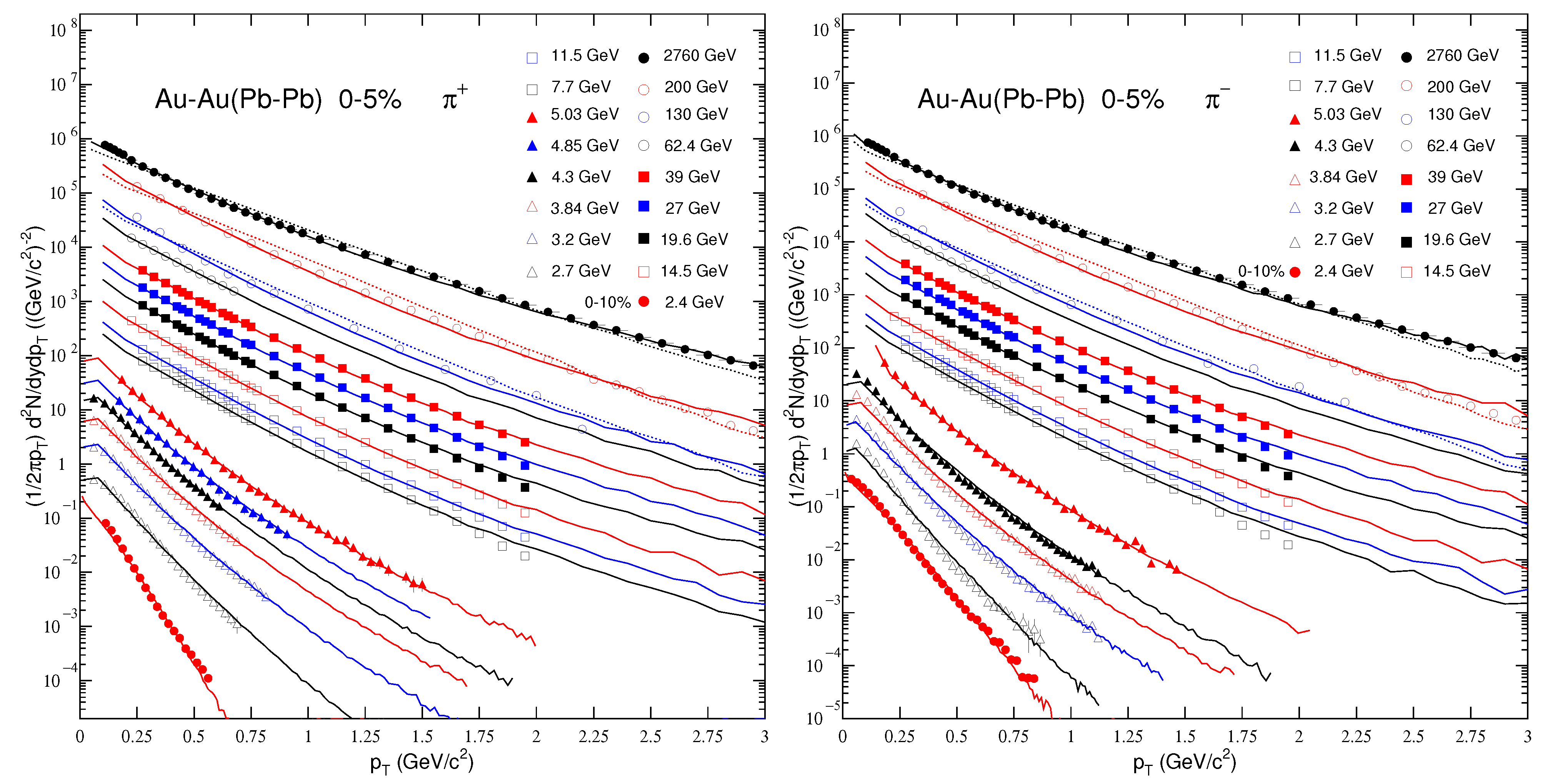
Figure 1 shows the $p_T$ spectra, invariant yield $(1/2\pi p_T)d^{2}N/dyd{p}_T$, of ${\pi }^{+}$ (left panel) and ${\pi }^{-}$ (right panel) produced at mid-y or mid-$\eta$ in central AA collisions. The experimental data (symbols) are from the HADES [16], E866 [18], E895 [20], STAR [23,24,25], PHENIX [28,29], and ALICE Collaborations [30,31]. Different symbols represent the data at different energies (2.4, 2.7, 3.2, 3.84, 4.3, 4.85, 5.03, 7.7, 11.5, 14.5, 19.6, 27, 39, 62.4, 130, 200, and 2760 GeV), where the centralities for 2.4 GeV and other energies are 0–10% and 0–5%, respectively. The solid curves represent the result of our fit by using the Monte Carlo method based on the modified Tsallis distribution. The dotted curves represent a few examples from the Tsallis distribution for comparisons. The energy 2760 GeV is for Pb-Pb collisions, while the others are for Au-Au collisions. What we need to emphasize here is that some data in the literature are given in the $m_T$ spectra which are converted by us to the $p_T$ spectra for the unification. To see the data clearly and keep them from the overlap, we multiply the data by the corresponding factors which are listed in

Table 1. Values of T, q, $a_0$, $N_0$, ${\chi }^2$, and ndof corresponding to the solid curves in Figure 1 in which ${\pi }^{+}$ (up panel) and ${\pi }^{-}$ (down panel) data are measured by different collaborations at different energies. Following the sets of parameters for the three top energies, the sets of parameters corresponding to the dotted curves are given.

Collab.	$\sqrt{{\mathit{s}}_{\mathbf{NN}}}$ (GeV)	Rapidity	Factor	T (GeV)	q	${\mathit{a}}_0$	${\mathit{N}}_0$	${\mathit{\chi }}^2$/ndof
HADES	2.4	$\left|y\right|<0.05$	5000	$0.062\pm 0.002$	$1.080\pm 0.002$	$-0.55\pm 0.02$	$(2.1\pm 0.1)\times {10}^{-6}$	$146/15$
E866	2.7	$\left|y\right|<0.05$	0.01	$0.130\pm 0.003$	$1.080\pm 0.004$	$-0.31\pm 0.06$	$12\pm 1$	$150/19$
E866	3.32	$\left|y\right|<0.05$	0.02	$0.153\pm 0.003$	$1.110\pm 0.004$	$-0.18\pm 0.06$	$29\pm 1$	$56/24$
E866	3.84	$\left|y\right|<0.05$	0.05	$0.162\pm 0.002$	$1.120\pm 0.003$	$-0.01\pm 0.02$	$39\pm 2$	$48/19$
E866	4.3	$\left|y\right|<0.05$	0.1	$0.164\pm 0.002$	$1.122\pm 0.005$	$-0.05\pm 0.02$	$48\pm 2$	$22/16$
E866	4.85	$\left|y\right|<0.05$	0.2	$0.170\pm 0.003$	$1.126\pm 0.006$	$-0.05\pm 0.04$	$52\pm 1$	$26/16$
E802	5.03	$\left|y\right|<0.2$	0.5	$0.176\pm 0.002$	$1.130\pm 0.006$	$-0.07\pm 0.03$	$55\pm 1$	$104/30$
STAR	7.7	$\left|y\right|<0.1$	0.8	$0.180\pm 0.001$	$1.130\pm 0.001$	$-0.07\pm 0.01$	$98\pm 2$	$41/22$
STAR	11.5	$\left|y\right|<0.1$	1	$0.180\pm 0.002$	$1.140\pm 0.002$	$-0.10\pm 0.02$	$131\pm 4$	$15/22$
STAR	14.5	$\left|y\right|<0.1$	2	$0.180\pm 0.002$	$1.142\pm 0.002$	$-0.10\pm 0.03$	$161\pm 2$	$3/24$
STAR	19.6	$\left|y\right|<0.1$	5	$0.184\pm 0.002$	$1.146\pm 0.004$	$-0.10\pm 0.04$	$169\pm 2$	$17/22$
STAR	27	$\left|y\right|<0.1$	10	$0.186\pm 0.001$	$1.146\pm 0.002$	$-0.10\pm 0.01$	$179\pm 3$	$9/21$
STAR	39	$\left|y\right|<0.1$	20	$0.189\pm 0.002$	$1.146\pm 0.003$	$-0.10\pm 0.03$	$189\pm 5$	$4/22$
STAR	62.4	$\left|y\right|<0.1$	50	$0.188\pm 0.003$	$1.144\pm 0.004$	$-0.11\pm 0.02$	$239\pm 2$	$1/6$
PHENIX	130	$\left|\eta \right|<0.35$	100	$0.183\pm 0.005$	$1.140\pm 0.005$	$-0.15\pm 0.03$	$253\pm 37$	$43/10$
				$0.153\pm 0.004$	$1.080\pm 0.003$		$253\pm 37$	$192/11$
PHENIX	200	$\left|\eta \right|<0.35$	400	$0.188\pm 0.003$	$1.143\pm 0.001$	$-0.05\pm 0.03$	$306\pm 12$	$108/24$
				$0.178\pm 0.005$	$1.043\pm 0.002$		$304\pm 12$	$561/25$
ALICE	2760	$\left|y\right|<0.5$	500	$0.227\pm 0.002$	$1.178\pm 0.002$	$-0.01\pm 0.01$	$750\pm 27$	$44/37$
				$0.187\pm 0.003$	$1.087\pm 0.001$		$750\pm 26$	$234/38$
HADES	2.4	$\left|y\right|<0.05$	3000	$0.078\pm 0.002$	$1.049\pm 0.002$	$-0.56\pm 0.02$	$(9.1\pm 0.1)\times {10}^{-5}$	$184/29$
E895	2.7	$\left|y\right|<0.05$	0.01	$0.110\pm 0.003$	$1.060\pm 0.004$	$-0.41\pm 0.06$	$19\pm 2$	$395/26$
E895	3.32	$\left|y\right|<0.05$	0.02	$0.143\pm 0.003$	$1.104\pm 0.004$	$-0.23\pm 0.06$	$38\pm 1$	$389/36$
E895	3.84	$\left|y\right|<0.05$	0.05	$0.150\pm 0.002$	$1.120\pm 0.003$	$-0.04\pm 0.02$	$48\pm 2$	$189/36$
E895	4.3	$\left|y\right|<0.05$	0.1	$0.155\pm 0.002$	$1.102\pm 0.005$	$-0.10\pm 0.02$	$62\pm 2$	$242/36$
E802	5.03	$0<y<0.4$	0.5	$0.170\pm 0.002$	$1.130\pm 0.006$	$-0.07\pm 0.03$	$64\pm 1$	$137/29$
STAR	7.7	$\left|y\right|<0.1$	0.8	$0.180\pm 0.001$	$1.128\pm 0.001$	$-0.07\pm 0.01$	$105\pm 3$	$75/22$
STAR	11.5	$\left|y\right|<0.1$	1	$0.177\pm 0.002$	$1.140\pm 0.002$	$-0.10\pm 0.02$	$137\pm 2$	$14/22$
STAR	14.5	$\left|y\right|<0.1$	2	$0.180\pm 0.002$	$1.142\pm 0.002$	$-0.10\pm 0.03$	$158\pm 3$	$5/24$
STAR	19.6	$\left|y\right|<0.1$	5	$0.184\pm 0.002$	$1.146\pm 0.004$	$-0.10\pm 0.04$	$170\pm 3$	$17/21$
STAR	27	$\left|y\right|<0.1$	10	$0.186\pm 0.001$	$1.146\pm 0.002$	$-0.10\pm 0.01$	$179\pm 3$	$12/22$
STAR	39	$\left|y\right|<0.1$	20	$0.189\pm 0.004$	$1.146\pm 0.003$	$-0.10\pm 0.02$	$189\pm 3$	$6/22$
STAR	62.4	$\left|y\right|<0.1$	50	$0.189\pm 0.003$	$1.144\pm 0.004$	$-0.11\pm 0.02$	$241\pm 10$	$1/6$
PHENIX	130	$\left|\eta \right|<0.35$	100	$0.186\pm 0.005$	$1.149\pm 0.005$	$-0.14\pm 0.03$	$231\pm 27$	$69/10$
				$0.153\pm 0.004$	$1.080\pm 0.002$		$231\pm 27$	$192/11$
PHENIX	200	$\left|\eta \right|<0.35$	400	$0.192\pm 0.003$	$1.143\pm 0.001$	$-0.05\pm 0.03$	$297\pm 18$	$114/24$
				$0.178\pm 0.004$	$1.043\pm 0.001$		$297\pm 17$	$478/25$
ALICE	2760	$\left|y\right|<0.5$	500	$0.227\pm 0.002$	$1.178\pm 0.002$	$-0.01\pm 0.01$	$738\pm 27$	$54/37$
				$0.187\pm 0.003$	$1.043\pm 0.002$		$738\pm 26$	$223/38$

.

In the process of fitting the data, we used the least square method to obtain the best parameters. The errors used to calculate ${\chi }^2$ are obtained by the root-mean-square of statistical and systematic errors. The parameters that minimize ${\chi }^2$ are the best parameters. The parameter errors are obtained by the statistical simulation method [53,54]. The collaborations, free parameters (T, q, and $a_0$), normalization factor ($N_0$), and number of degree-of-freedom (ndof) are listed in Table 1. From the comparisons between the solid and dotted curves in Figure 1 and between the two sets of ${\chi }^2$ in Table 1, one can see that the modified Tsallis distribution is better than the Tsallis distribution in the fit. In view of these comparisons, we give up using the Tsallis distribution in the fit for other data.

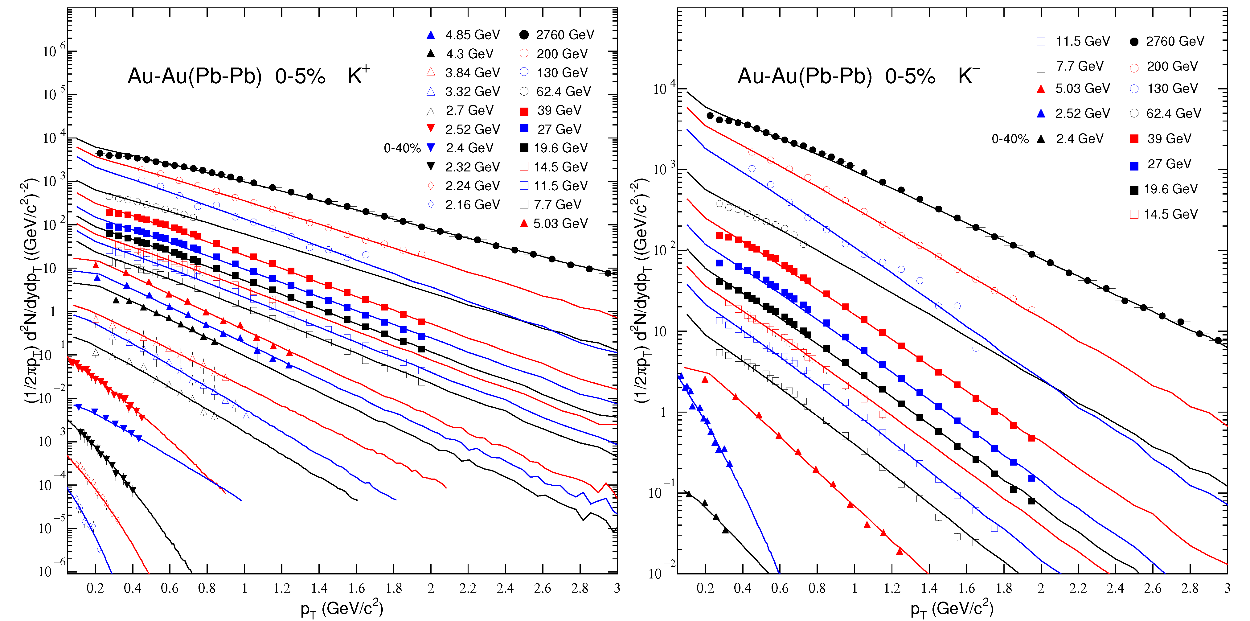
Figure 2 is similar to Figure 1, but it shows the invariant yield of $K^{+}$ (left panel) and $K^{-}$ (right panel) produced at mid-y or mid-$\eta$ in central Au-Au and Pb-Pb collisions. The data are from the KaoS [15], HADES [16], E866 [18], E802 [21], STAR [23,24,25], PHENIX [28,29], and ALICE Collaborations [30,31] over an energy range from 2.16 to 2760 GeV, where the centralities for 2.4 GeV and other energies are 0–40% and 0–5%, respectively (0–5.4% for 2.16, 2.24, 2.32, and 2.52 GeV, which is not marked in the panels). To see the data clearly and keep them from the overlap, we multiply the data by the corresponding factors. Similarly, the collaborations, T, q, $a_0$, $N_0$, and ndof are listed in

Table 2. Values of T, q, $a_0$, $N_0$, ${\chi }^2$, and ndof corresponding to the curves in Figure 2 in which $K^{+}$ (up panel) and $K^{-}$ (down panel) data are measured by different collaborations at different energies. In one case, ndof is less than 1, which is denoted by − in the table, and the corresponding curve is obtained by an extrapolation.

Collab.	$\sqrt{{\mathit{s}}_{\mathbf{NN}}}$ (GeV)	Rapidity	Factor	T (GeV)	q	${\mathit{a}}_0$	${\mathit{N}}_0$	${\mathit{\chi }}^2$/ndof
KaoS	2.16	$\left|y\right|<0.5$	0.1	$0.020\pm 0.002$	$1.002\pm 0.003$	$-0.56\pm 0.05$	$(4.3\pm 0.1)\times {10}^{-5}$	$4/3$
KaoS	2.24	$\left|y\right|<0.5$	0.05	$0.037\pm 0.002$	$1.004\pm 0.003$	$-0.46\pm 0.05$	$(7.3\pm 0.1)\times {10}^{-4}$	$2/6$
KaoS	2.32	$\left|y\right|<0.5$	0.1	$0.052\pm 0.002$	$1.004\pm 0.003$	$-0.46\pm 0.05$	$(3.3\pm 0.1)\times {10}^{-3}$	$1/8$
HADES	2.4	$\left|y\right|<0.1$	$5\times {10}^{10}$	$0.154\pm 0.004$	$1.010\pm 0.005$	$0.56\pm 0.05$	$(2.1\pm 0.1)\times {10}^{-13}$	$7/3$
KaoS	2.52	$\left|y\right|<0.5$	0.3	$0.089\pm 0.002$	$1.014\pm 0.003$	$-0.36\pm 0.05$	$0.5\pm 0.3$	$4/16$
E866	2.7	$\left|y\right|<0.23$	1	$0.159\pm 0.004$	$1.010\pm 0.005$	$0.56\pm 0.05$	$0.40\pm 0.03$	$67/6$
E866	3.32	$\left|y\right|<0.29$	0.5	$0.160\pm 0.002$	$1.010\pm 0.005$	$0.53\pm 0.02$	$2.60\pm 0.09$	$45/8$
E866	3.84	$\left|y\right|<0.05$	0.5	$0.189\pm 0.002$	$1.029\pm 0.002$	$0.69\pm 0.01$	$5.40\pm 0.09$	$34/7$
E866	4.3	$\left|y\right|<0.05$	1.5	$0.195\pm 0.001$	$1.031\pm 0.003$	$0.72\pm 0.02$	$8.8\pm 0.2$	$25/5$
E866	4.85	$\left|y\right|<0.2$	2	$0.198\pm 0.005$	$1.033\pm 0.003$	$0.72\pm 0.02$	$13\pm 1$	$31/7$
E802	5.03	$0<y<0.4$	4	$0.199\pm 0.002$	$1.034\pm 0.001$	$0.73\pm 0.03$	$13\pm 1$	$32/7$
STAR	7.7	$\left|y\right|<0.1$	1	$0.197\pm 0.002$	$1.033\pm 0.003$	$0.72\pm 0.05$	$23\pm 1$	$40/19$
STAR	11.5	$\left|y\right|<0.1$	1.5	$0.197\pm 0.001$	$1.033\pm 0.002$	$0.72\pm 0.01$	$27\pm 1$	$32/21$
STAR	14.5	$\left|y\right|<0.1$	2	$0.203\pm 0.002$	$1.036\pm 0.004$	$0.74\pm 0.03$	$31\pm 1$	$1/14$
STAR	19.6	$\left|y\right|<0.1$	3	$0.203\pm 0.001$	$1.036\pm 0.002$	$0.74\pm 0.03$	$31\pm 1$	$16/22$
STAR	27	$\left|y\right|<0.1$	5	$0.207\pm 0.002$	$1.037\pm 0.003$	$0.79\pm 0.03$	$32\pm 1$	$39/22$
STAR	39	$\left|y\right|<0.1$	10	$0.207\pm 0.002$	$1.037\pm 0.003$	$0.79\pm 0.04$	$34\pm 1$	$29/22$
STAR	62.4	$\left|y\right|<0.1$	20	$0.229\pm 0.002$	$1.042\pm 0.001$	$0.99\pm 0.01$	$42\pm 1$	$8/6$
PHENIX	130	$\left|\eta \right|<0.35$	50	$0.207\pm 0.005$	$1.037\pm 0.006$	$0.79\pm 0.05$	$46\pm 6$	$11/9$
PHENIX	200	$\left|\eta \right|<0.35$	100	$0.227\pm 0.003$	$1.042\pm 0.002$	$0.99\pm 0.05$	$49\pm 3$	$15/12$
ALICE	2760	$\left|y\right|<0.5$	100	$0.242\pm 0.002$	$1.062\pm 0.002$	$1.39\pm 0.02$	$114\pm 4$	$25/32$
HADES	2.4	$\left|y\right|<0.05$	$5\times {10}^{13}$	$0.154\pm 0.004$	$1.010\pm 0.005$	$0.56\pm 0.05$	$(3.2\pm 0.1)\times {10}^{-15}$	$4/-$
KaoS	2.52	$\left|y\right|<0.5$	500	$0.063\pm 0.002$	$1.010\pm 0.003$	$-0.46\pm 0.05$	$(6.6\pm 0.1)\times {10}^{-3}$	$11/79$
E802	5.03	$\left|y\right|<0.1$	4	$0.193\pm 0.002$	$1.031\pm 0.001$	$0.66\pm 0.03$	$2.5\pm 0.0$	$34/37$
STAR	7.7	$\left|y\right|<0.1$	1	$0.190\pm 0.002$	$1.030\pm 0.003$	$0.68\pm 0.05$	$8.3\pm 0.2$	$43/19$
STAR	11.5	$\left|y\right|<0.1$	1.5	$0.190\pm 0.001$	$1.030\pm 0.002$	$0.70\pm 0.01$	$13\pm 1$	$27/19$
STAR	14.5	$\left|y\right|<0.1$	2	$0.200\pm 0.002$	$1.035\pm 0.004$	$0.72\pm 0.03$	$18\pm 1$	$1/14$
STAR	19.6	$\left|y\right|<0.1$	3	$0.201\pm 0.001$	$1.034\pm 0.002$	$0.73\pm 0.03$	$20\pm 2$	$15/22$
STAR	27	$\left|y\right|<0.1$	5	$0.200\pm 0.002$	$1.032\pm 0.003$	$0.75\pm 0.03$	$24\pm 1$	$30/20$
STAR	39	$\left|y\right|<0.1$	10	$0.208\pm 0.002$	$1.037\pm 0.003$	$0.79\pm 0.04$	$27\pm 1$	$20/22$
STAR	62.4	$\left|y\right|<0.1$	20	$0.230\pm 0.002$	$1.042\pm 0.001$	$0.99\pm 0.01$	$38\pm 1$	$22/6$
PHENIX	130	$\left|\eta \right|<0.35$	50	$0.204\pm 0.005$	$1.033\pm 0.006$	$0.76\pm 0.05$	$38\pm 6$	$9/9$
PHENIX	200	$\left|\eta \right|<0.35$	100	$0.227\pm 0.003$	$1.042\pm 0.002$	$0.99\pm 0.05$	$46\pm 5$	$11/12$
ALICE	2760	$\left|y\right|<0.5$	100	$0.247\pm 0.002$	$1.052\pm 0.002$	$1.39\pm 0.02$	$110\pm 4$	$15/32$

with the factors.

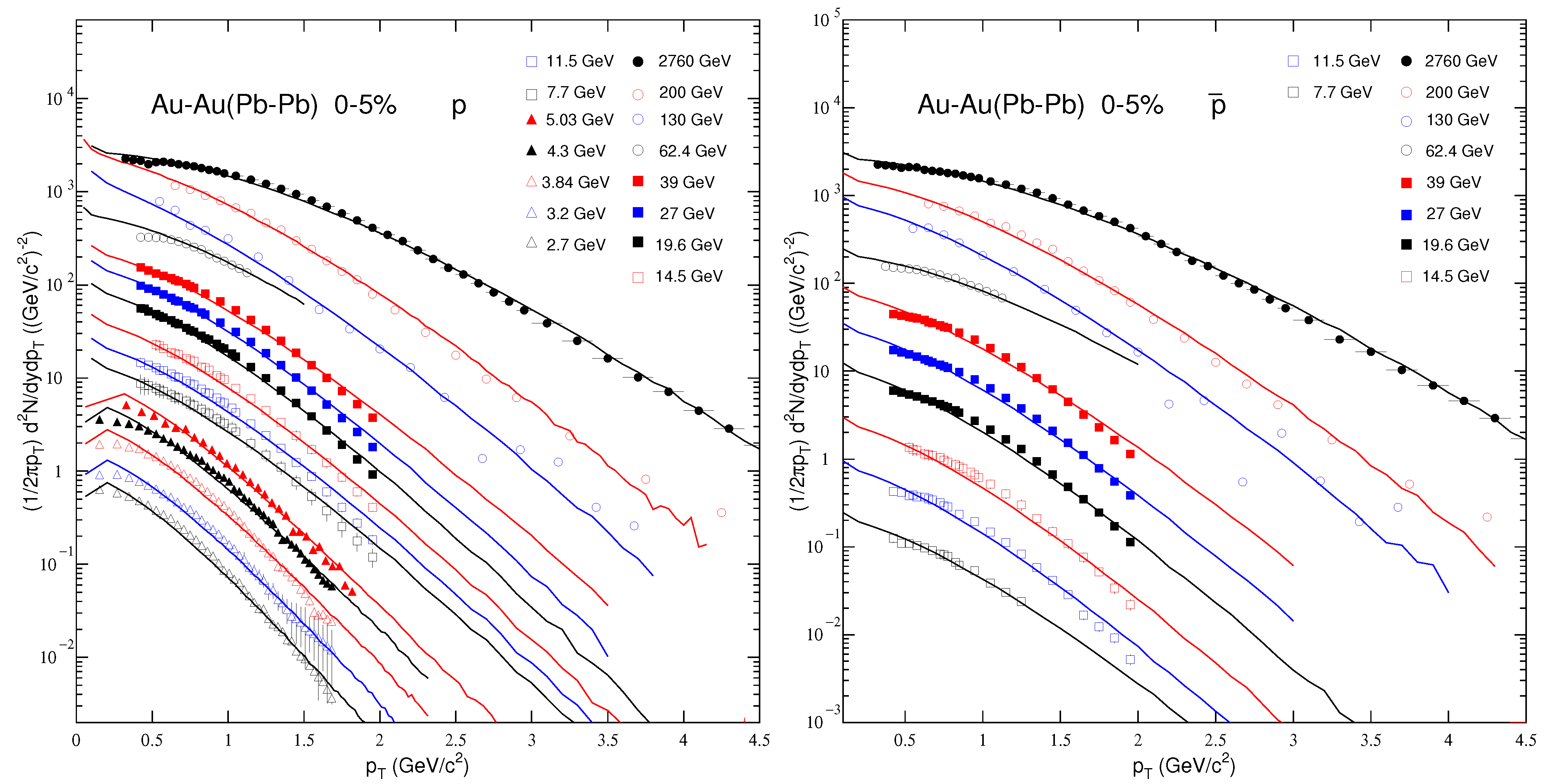
Figure 3 is similar to Figure 1 and Figure 2, but it shows the invariant yield of p (left panel) and $\overline{p}$ (right panel) produced at mid-y or mid-$\eta$ in 0–5% Au-Au and Pb-Pb collisions. The data are from the E895 [19], E802 [22], STAR [23,24,25], PHENIX [28,29], and ALICE Collaborations [30,31] in the energy range of 2.7–2760 GeV. To see the data clearly and keep them from the overlap, we multiply the data by the corresponding factors. Similarly, the collaborations, T, q, $a_0$, $N_0$, and ndof are listed in

Table 3. Values of T, q, $a_0$, $N_0$, ${\chi }^2$, and ndof corresponding to the curves in Figure 3 in which p (up panel) and $\overline{p}$ (down panel) data are measured by different collaborations at different energies.

Collab.	$\sqrt{{\mathit{s}}_{\mathbf{NN}}}$ (GeV)	Rapidity	Factor	T (GeV)	q	${\mathit{a}}_0$	${\mathit{N}}_0$	${\mathit{\chi }}^2$/ndof
E895	2.7	$\left|y\right|<0.05$	0.1	$0.180\pm 0.003$	$1.005\pm 0.004$	$1.35\pm 0.08$	$75\pm 6$	$256/36$
E895	3.32	$\left|y\right|<0.05$	0.2	$0.187\pm 0.003$	$1.008\pm 0.005$	$1.38\pm 0.08$	$71\pm 5$	$217/36$
E895	3.84	$\left|y\right|<0.34$	0.5	$0.193\pm 0.002$	$1.008\pm 0.002$	$1.38\pm 0.05$	$64\pm 6$	$309/36$
E895	4.3	$\left|y\right|<0.37$	1	$0.199\pm 0.004$	$1.011\pm 0.002$	$1.42\pm 0.06$	$60\pm 4$	$236/36$
E802	5.03	$\left|y\right|<0.1$	1.5	$0.199\pm 0.001$	$1.013\pm 0.002$	$1.44\pm 0.06$	$69\pm 2$	$465/25$
STAR	7.7	$\left|y\right|<0.1$	0.5	$0.204\pm 0.001$	$1.010\pm 0.003$	$1.44\pm 0.02$	$56\pm 1$	$48/25$
STAR	11.5	$\left|y\right|<0.1$	1	$0.204\pm 0.001$	$1.010\pm 0.002$	$1.44\pm 0.04$	$46\pm 2$	$61/24$
STAR	14.5	$\left|y\right|<0.1$	2	$0.204\pm 0.001$	$1.010\pm 0.003$	$1.44\pm 0.04$	$42\pm 1$	$6/21$
STAR	19.6	$\left|y\right|<0.1$	5	$0.205\pm 0.002$	$1.010\pm 0.002$	$1.44\pm 0.06$	$36\pm 1$	$24/25$
STAR	27	$\left|y\right|<0.1$	10	$0.209\pm 0.002$	$1.010\pm 0.002$	$1.44\pm 0.07$	$33\pm 1$	$15/19$
STAR	39	$\left|y\right|<0.1$	20	$0.219\pm 0.001$	$1.010\pm 0.001$	$1.47\pm 0.02$	$27\pm 1$	$17/18$
STAR	62.4	$\left|y\right|<0.1$	50	$0.239\pm 0.002$	$1.009\pm 0.004$	$1.87\pm 0.04$	$34\pm 1$	$46/11$
PHENIX	130	$\left|\eta \right|<0.35$	100	$0.223\pm 0.002$	$1.020\pm 0.002$	$1.51\pm 0.05$	$28\pm 1$	$629/13$
PHENIX	200	$\left|\eta \right|<0.35$	400	$0.233\pm 0.001$	$1.003\pm 0.001$	$1.71\pm 0.02$	$17\pm 1$	$83/18$
ALICE	2760	$\left|y\right|<0.5$	500	$0.263\pm 0.001$	$1.003\pm 0.002$	$2.21\pm 0.05$	$33\pm 2$	$102/38$
STAR	7.7	$\left|y\right|<0.1$	1	$0.208\pm 0.001$	$1.013\pm 0.003$	$1.47\pm 0.02$	$0.40\pm 0.01$	$5/11$
STAR	11.5	$\left|y\right|<0.1$	1	$0.200\pm 0.001$	$1.010\pm 0.002$	$1.40\pm 0.04$	$1.50\pm 0.03$	$57/19$
STAR	14.5	$\left|y\right|<0.1$	2	$0.201\pm 0.001$	$1.010\pm 0.003$	$1.44\pm 0.04$	$2.5\pm 0.2$	$8/21$
STAR	19.6	$\left|y\right|<0.1$	5	$0.204\pm 0.002$	$1.010\pm 0.002$	$1.44\pm 0.06$	$4.2\pm 0.1$	$31/18$
STAR	27	$\left|y\right|<0.1$	10	$0.209\pm 0.002$	$1.010\pm 0.002$	$1.44\pm 0.07$	$6.4\pm 0.1$	$22/18$
STAR	39	$\left|y\right|<0.1$	20	$0.217\pm 0.001$	$1.010\pm 0.001$	$1.47\pm 0.02$	$9.0\pm 0.1$	$320/19$
STAR	62.4	$\left|y\right|<0.1$	50	$0.239\pm 0.002$	$1.009\pm 0.004$	$1.87\pm 0.04$	$17\pm 1$	$18/12$
PHENIX	130	$\left|\eta \right|<0.35$	100	$0.233\pm 0.002$	$1.007\pm 0.002$	$1.51\pm 0.05$	$21\pm 1$	$23/13$
PHENIX	200	$\left|\eta \right|<0.35$	400	$0.233\pm 0.001$	$1.003\pm 0.001$	$1.71\pm 0.02$	$12\pm 1$	$60/18$
ALICE	2760	$\left|y\right|<0.5$	500	$0.263\pm 0.001$	$1.003\pm 0.002$	$2.21\pm 0.05$	$33\pm 2$	$111/38$

with the factors.

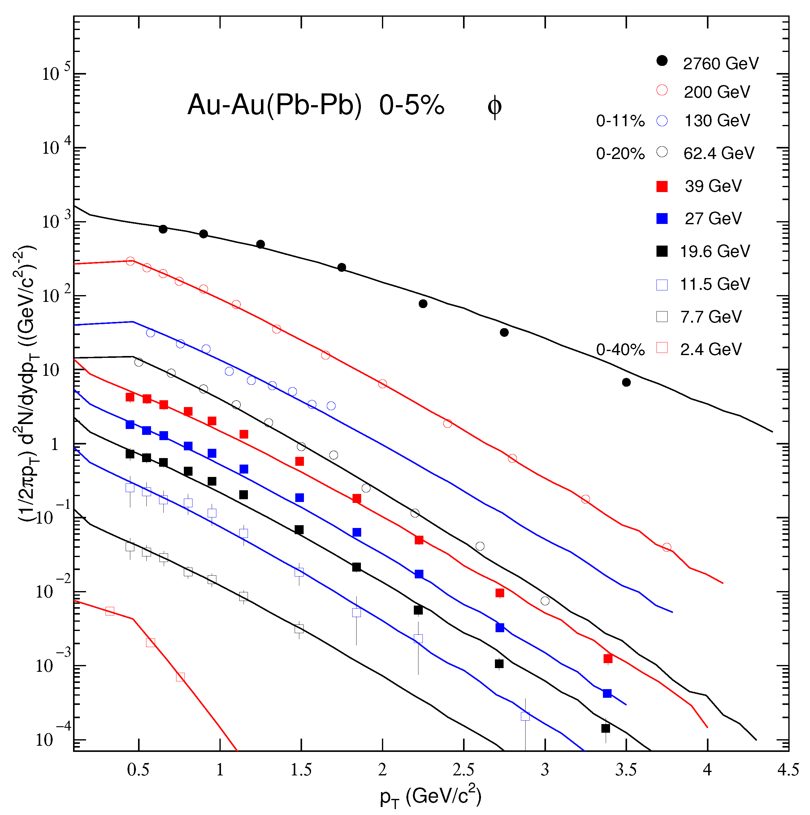
Figure 4 is similar to Figure 1, Figure 2 and Figure 3, but it shows the invariant yield of $\varphi$ produced at mid-y in central Au-Au and Pb-Pb collisions. The data are from the HADES [17], STAR [26,27], and ALICE Collaborations [32]. The energies are 2.4, 7.7, 11.5, 19.6, 27, 39, 62.4, 130, 200, and 2760 GeV, where the centralities for 2.4, 62.4, and 130 GeV are 0–40%, 0–20%, and 0–11%, respectively, and for other energies are 0–5%. To see the data clearly and keep them from the overlap, we multiply the data by the corresponding factors. Similarly, the collaborations, T, q, $a_0$, $N_0$, and ndof are listed in

Table 4. Values of T, q, $a_0$, $N_0$, ${\chi }^2$, and ndof corresponding to the curves in Figure 4 in which $\varphi$ data are measured by different collaborations at different energies. In one case, ndof is less than 1, which is denoted by - in the table, and the corresponding curve is obtained by an extrapolation.

Collab.	$\sqrt{{\mathit{s}}_{\mathbf{NN}}}$ (GeV)	Rapidity	Factor	T (GeV)	q	${\mathit{a}}_0$	${\mathit{N}}_0$	${\mathit{\chi }}^2$/ndof
HADES	2.4	$\left|y\right|<0.1$	$1\times {10}^{14}$	$0.124\pm 0.001$	$1.002\pm 0.001$	$0.60\pm 0.06$	$(6.8\pm 0.1)\times {10}^{-16}$	3/-
STAR	7.7	$\left|y\right|<0.5$	0.1	$0.244\pm 0.002$	$1.009\pm 0.001$	$1.40\pm 0.03$	$1.4\pm 0.1$	$10/3$
STAR	11.5	$\left|y\right|<0.5$	0.5	$0.242\pm 0.001$	$1.006\pm 0.001$	$1.30\pm 0.01$	$1.8\pm 0.1$	$7/6$
STAR	19.6	$\left|y\right|<0.5$	1	$0.247\pm 0.001$	$1.006\pm 0.001$	$1.40\pm 0.02$	$2.5\pm 0.2$	$15/7$
STAR	27	$\left|y\right|<0.5$	2	$0.247\pm 0.001$	$1.006\pm 0.001$	$1.40\pm 0.06$	$3.0\pm 0.4$	$10/8$
STAR	39	$\left|y\right|<0.5$	5	$0.251\pm 0.002$	$1.006\pm 0.001$	$1.50\pm 0.07$	$3.3\pm 0.3$	$1/8$
STAR	62.4	$\left|y\right|<0.5$	100	$0.251\pm 0.003$	$1.006\pm 0.001$	$1.80\pm 0.06$	$3.8\pm 0.4$	$10/7$
STAR	130	$\left|y\right|<0.5$	200	$0.261\pm 0.003$	$1.006\pm 0.001$	$2.00\pm 0.07$	$6.3\pm 0.2$	$5/5$
STAR	200	$\left|y\right|<0.5$	1000	$0.261\pm 0.001$	$1.006\pm 0.001$	$2.00\pm 0.06$	$8.4\pm 0.5$	$8/10$
ALICE	2760	$\left|y\right|<0.5$	500	$0.281\pm 0.001$	$1.012\pm 0.001$	$2.90\pm 0.06$	$14\pm 1$	$1/4$

with the factors.

One can see from Figure 1, Figure 2, Figure 3 and Figure 4 and Table 1, Table 2, Table 3 and Table 4 that our results by the Monte Carlo method describe approximately the tendency of the considered experimental data. In our work, due to the narrow range of $p_T$ spectra being used, we have considered only two participant partons and one component (temperature). It is natural and easy that we can extend this work to three or more participant partons and two or more components (temperatures) if needed. In the Monte Carlo calculations, adding the contributions of more participant partons means increasing the number of items in Equations (7) and (8), while adding more components (temperatures) means increasing new Equations (7) and (8) with different temperatures in the calculations and different proportions in the statistics.

3.2. Tendency of Parameters and Discussion

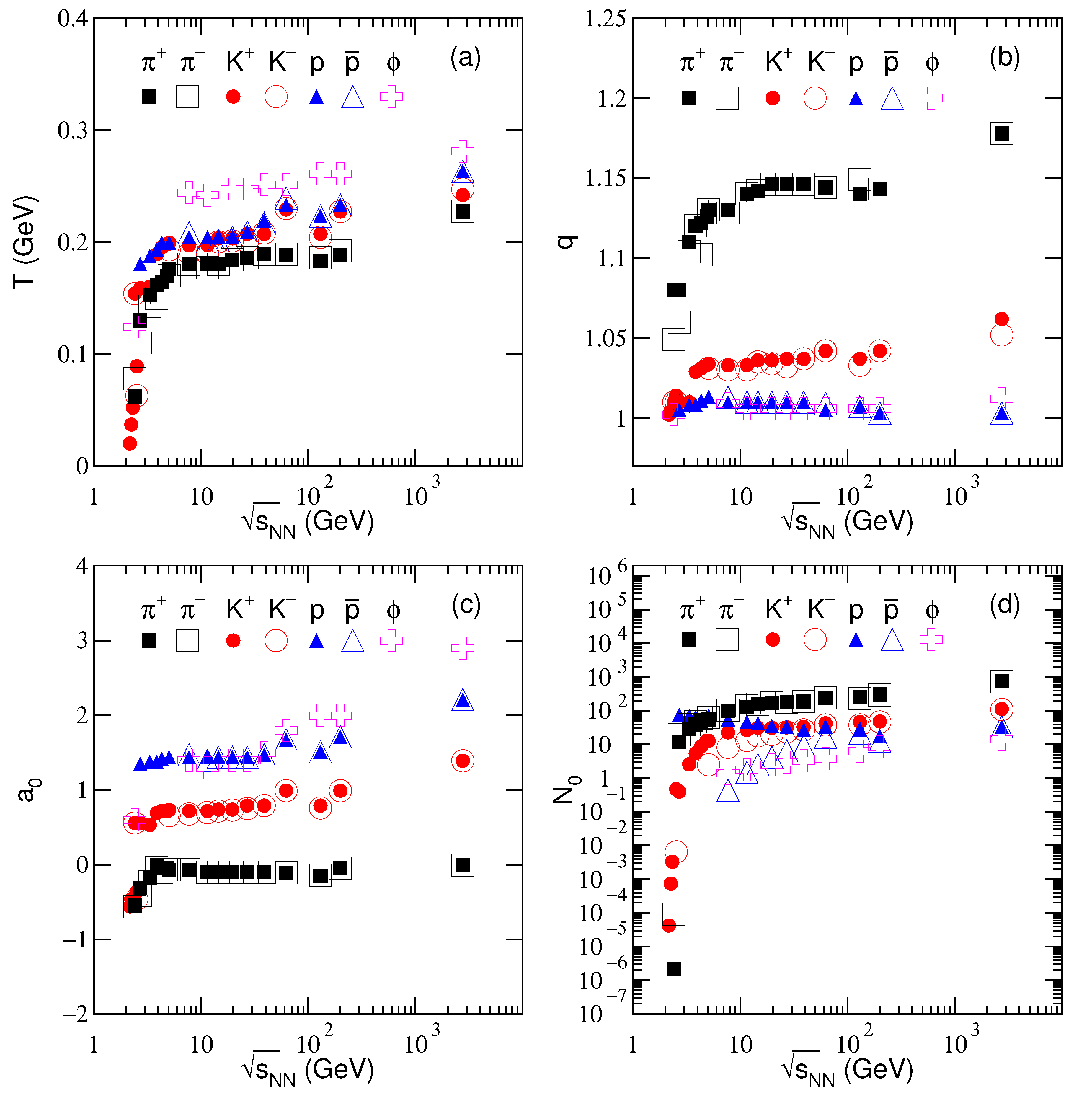
In order to study the change trend of parameters, Figure 5 shows the dependences of (a) T, (b) q, (c) $a_0$, and (d) $N_0$ on collision energy $\sqrt{s_{NN}}$. In the figure, the squares, circles, triangles, and crosses represent the results from the ${\pi }^{\pm }$, $K^{\pm }$, $p\left(\overline{p}\right)$, and $\varphi$ spectra, respectively. The closed symbols indicate the positive particles, and the open ones indicate the negative particles. From Figure 5, one can see that, as $\sqrt{s_{NN}}$ increases, the parameter T increases quickly from 2.16 to 5 GeV and then slightly from 5 to 2760 GeV in the results from ${\pi }^{\pm }$ and $K^{\pm }$ spectra. The parameter q for ${\pi }^{\pm }$ increases quickly and then slowly around 5 GeV, and for $K^{\pm }$ and $p\left(\overline{p}\right)$ shows a slight increase. The parameter $a_0$ shows a slight increase or remains almost unchanged in most cases. The parameter $N_0$ decreases for p and increases quickly and then slowly around 5 GeV for ${\pi }^{\pm }$ and $K^{\pm }$. These parameters also show the particle mass dependent. That is, with the increase of particle mass, T and $a_0$ increase and q and $N_0$ decrease in most cases.

We call T the effective temperature due to the fact that it contains the contributions of thermal motion described by the kinetic freeze-out temperature, $T_0$, and flow effect described by the average transverse flow velocity, $\langle {\beta }_T\rangle$. To relate the obtained T to the expected $T_0$ and ${\beta }_T$, one may consider a possible relation, $T_0=\langle p_T\rangle /3.07$ [55], where $\langle p_T\rangle$ is the average $p_T$, which can be obtained from the statistics in which T, q, and $a_0$ play important roles. Then, we have $\langle {\beta }_T\rangle =(2.07/3.07)\langle p_T\rangle /\overline{m}$, where $\overline{m}$ is the average energy (average moving mass) of the considered particle in the source rest frame. It is regretful that we have no idea to establish the linkage between T ($T_0$) and the phase transition temperature at present. In addition, T from different distributions (or functions or models) are different in their sizes, though the trends are similar or compatible [15,16,17].

There is a possible situation on the relation between $T_0$ and $\langle {\beta }_T\rangle$, which satisfies the hydrodynamics in which $T_0$ increases and $\langle {\beta }_T\rangle$ decreases with the increase of particle mass. This is due to the early leaving over for the massive particles during the evolution of the system. The mass dependent T reflects mainly the influence of flow effect which shows a decreasing $\langle {\beta }_T\rangle$ with the increase of mass. Although the contributions of $T_0$ and $\langle {\beta }_T\rangle$ in T are not dissociated in the present work, we may obtain a definite T, which is not different from the indefinite $T_0$ and $\langle {\beta }_T\rangle$ due to different dissociated methods being used.

The boundary (5 GeV) from the quick to slow increases of T reflects the change of reaction mechanism and/or generated matter. There are two possible situations: (i) The products of the system experience a change from baryon-dominated to meson-dominated, where the hadron phase or nuclear matter always exists; (ii) The system undergoes the de-confined phase transition from nuclear matter to QGP. Indeed, a few GeV energy range is very important due to it containing abundant information. This energy range covers the initial energy of limiting fragmentation of nuclei, the critical energy of possible change from baryon-dominated to meson-dominated, and the critical energy of a possible de-confined phase transition. Anyhow, the boundary should be given more attention in the future study.

The entropy index q reflects the degree of equilibrium or non-equilibrium of the collision system. The system reaches the equilibrium state at $q=1$, while $q\gg 1$ (e.g., $q>1.25$) represents a non-equilibrium state. In our work, q is close to 1, which shows that the equilibrium is basically maintained. Usually, the equilibrium is relative. For an approximate equilibrium situation, we can also use the concept of local equilibrium for different local parts. If q is not too large, for example, $q\le 1.25$, the collision system is in approximate equilibrium or local equilibrium [34,56].

As can be seen from Figure 5, q values are the highest for pions. However, the pion production is the highest in AA collisions and one would expect that they would reach equilibrium faster, which should result in low q. However, in the collisions, the excitation of pions is also the highest due to their small mass. This means that pions are possibly further away from the equilibrium of original partons than other particles, which results in high values of q for pions.

Because of most protons coming directly from the participant nuclei, they have enough time to reach equilibrium during their evolution. This also renders that q is closer to 1 for emission of protons. Our results show that q increases with an increase in the energy. At lower energy, the system is closer to the equilibrium state because the lower energy evolution process is slower, and the system has more time to reach equilibrium. From initial collision to kinetic freeze-out, the evolution time is very short. We have consistent results: the lower the collision energy, the longer the evolution time, the closer to 1 the q, and the more equilibrium the system has. Our results show indeed a q closer to 1 at lower energy.

The parameter $a_0$ reflects the shape of a particle spectrum in a low-$p_T$ region. If $a_0=1$ corresponds to a normal shape of the spectrum, $a_0<1$ means a rising tendency and $a_0>1$ means a falling tendency of the spectrum. Due to the constraint of normalization, $a_0$ also affects the tendency of the spectrum in intermediate- and high-$p_T$ regions, though it determines mainly the tendency in low-$p_T$ region. The introduction of $a_0$ results in the fit process being more flexible, though one more parameter is introduced. Although $a_0$ is dimensionless, its introduction causes the dimension of $m_{T_i}$ to that of $m_{T_i}^{a_0}$. This can be adjusted by the normalization constant C so that the probability density function is still workable. Meanwhile, in Equations (1)–(3), the power $-q/(q-1)$ determines the thermodynamic consistency. The inconsistency or approximate consistency caused by $a_0$ may be also adjusted by the normalization constant.

The fact that $a_0\ne 1$ means that the introduction of $a_0$ is necessary. Our results show that $a_0$ is less than and close to 0 in most cases for the production of ${\pi }^{\pm }$, around 1 for the production of $K^{\pm }$, around 1.5 for the production of $p\left(\overline{p}\right)$, and around 1.5–3 for the production of $\varphi$. Although the meaning of difference in $a_0$ for different particles is not very clear for us, $a_0<1$ for the production of ${\pi }^{\pm }$ renders the contribution of resonance as significant, $a_0\approx 1$ for the production of $K^{\pm }$ renders that the contribution of resonance is not too large, and their production is not restrained, while $a_0>1$ for the production of $p\left(\overline{p}\right)$ and $\varphi$ means that their productions are restrained. From low energy to high ones, $a_0$ has slight fluctuations for given particles in most cases. This is a reflection of the same or similar shape of the spectrum in a low-$p_T$ region for given particles in the considered energy range.

Generally, with increasing $\sqrt{s_{NN}}$, $N_0$ increases quickly and then slowly for produced particles which does not include p. It is understandable that more energies are deposited in the collisions at higher energy. Then, more particles are produced due to the fact that the deposited energies are transformed to masses due to the conservation of energy. The situation of p is different. As a component of projectile and target nuclei, p will be lost due to the collisions. The higher the energy is, the more it is lost. The loss of p will cause the increase of other baryons due to the conversation of baryon number. The increasing $N_0$ for produced particles also reflects the increasing volume of the system.

For the most abundant produced particles, ${\pi }^{\pm }$ yield increases quickly and then slowly. The boundary is around 5 GeV. With increasing the mass, the boundary increases. This depends on the threshold energy required for particle generation. Generally, the average parameter is obtained by weighting the yields of different particles. Because of the most abundant produced particles being ${\pi }^{\pm }$ in collisions at high energy, the average parameter is approximately determined by that for ${\pi }^{\pm }$. Considering the massive yield of p at low energy, the average parameter is approximately determined by those for ${\pi }^{\pm }$ and p.

To obtain an average parameter more accurately, one may consider ${\pi }^{\pm }$, $K^{\pm }$, $p\left(\overline{p}\right)$, and other particles together. The average parameters can be approximately used to fit the spectra of different particles. In this case, the productions of different particles are regarded as the result of simultaneous decay of the system. Obviously, the application of average parameters covers the mass dependent scenario, which reflects the fine structure of the system evolution. In our opinion, the decay of the system is not simultaneously. The massive particles are produced early because they are left over in the hydrodynamics of the system evolution.

Before summary and conclusions, we would like to point out that the chemical potential mentioned in Equations (1)–(4) can be neglected at high energy such as dozens of GeV and above. That is to say that the chemical potential is redundant at high energy [57]. However, the chemical potential is sizeable at low energy such as a few GeV, though its influence is still small. At low energy, the temperature values from the spectra of different particles overlap each other, as what we observed in Figure 5a. The situations of temperature values are nearly the same if we consider the two cases of ${\mu }_{u,d}=0$ and ${\mu }_{u,d}={\mu }_B/3$ [36]. The nearly independent of chemical potential renders that it is also redundant at low energy [57].

In addition, the influence of q on the spectra in high-$p_T$ region at both the low and high energies is also remarkable. This is not surprising that a slight increase of q value can result in a large increase in the high-$p_T$ region, while the values of other parameters may remain nearly invariant. Because the value of q is close to 1, we may still say that the system stays in approximate or local equilibrium, though a large difference of the spectra in high-$p_T$ region is observed between the equilibrium and approximate or local equilibrium. In our opinion, the approximate or local equilibrium is achieved in the considered collisions.

4. Summary and Conclusions

We summarize here our main observations and conclusions:

(a)

We have used a new method to analyze the $p_T$ spectra of identified particles produced in central AA collisions. The particle’s $p_T$ is regarded as the joint contribution of two participant partons which obey the modified Tsallis-like transverse momentum distribution and have random azimuths in superposition. The Monte Carlo method is performed to calculate and fit the experimental $p_T$ spectra of ${\pi }^{\pm }$, $K^{\pm }$, $p\left(\overline{p}\right)$, and $\varphi$ produced in central Au-Au and Pb-Pb collisions over an energy range from 2.16 to 2760 GeV measured by international collaborations. Three free parameters, the effective temperature T, entropy index q, and revised index $a_0$ are obtained.

(b)

Our results show that, with the increase of $\sqrt{s_{NN}}$, T increases quickly and then slowly in the results from ${\pi }^{\pm }$ and $K^{\pm }$ spectra. The boundary is around 5 GeV. This energy is possibly the critical energy of a possible de-confined phase transition from hadron matter to QGP. The values of q are close to 1 and have a slight increase with increasing $\sqrt{s_{NN}}$. This result shows that the system is in approximate equilibrium in the considered energy range and closer to the equilibrium at lower energy. Generally, the values of $a_0$ are mass dependent and not energy dependent. The resonance generation of ${\pi }^{\pm }$ and the constraints of other particles in a low-$p_T$ region are reflected by the values of $a_0$.

References

- Flor, F.A.; Olinger, G.; Bellwied, R. System size and flavour dependence of chemical freeze-out temperatures in ALICE pp, pPb and PbPb collisions at LHC energies. arXiv 2021, arXiv:2109.09843. [Google Scholar]
- Lu, Y.; Chen, M.Y.; Bai, Z.; Gao, F.; Liu, Y.-X. Chemical freeze-out parameters via a non-perturbative QCD approach. arXiv 2019, arXiv:2109.09912. [Google Scholar]
- Motornenko, A.; Steinheimer, J.; Vovchenko, V.; Stock, R.; Stoecker, H. Ambiguities in the hadro-chemical freeze-out of Au+Au collisions at SIS18 energies and how to resolve them. Phys. Lett. B 2021, 822, 136703. [Google Scholar] [CrossRef]
- Tang, Z.B.; Xu, Y.C.; Ruan, L.J.; van Buren, G.; Wang, F.Q.; Xu, Z.B. Spectra and radial flow at RHIC with Tsallis statistics in a blast-wave description. Phys. Rev. C 2009, 79, 051901. [Google Scholar] [CrossRef] [Green Version]
- Chatterjee, S.; Das, S.; Kumar, L.; Mishra, D.; Mohanty, B.; Sahoo, R.; Sharma, N. Freeze-out parameters in heavy-ion collisions at AGS, SPS, RHIC, and LHC energies. Adv. High Energy Phys. 2015, 2015, 349013. [Google Scholar] [CrossRef]
- Chatterjee, S.; Mohanty, B.; Singh, R. Freezeout hypersurface at energies available at the CERN Large Hadron Collider from particle spectra: Flavor and centrality dependence. Phys. Rev. C 2015, 92, 024917. [Google Scholar] [CrossRef]
- Waqas, M.; Peng, G.X.; Liu, F.-H. An evidence of triple kinetic freezeout scenario observed in all centrality intervals in Cu–Cu, Au–Au and Pb–Pb collisions at high energies. J. Phys. G 2021, 48, 075108. [Google Scholar] [CrossRef]
- Waqas, M.; Liu, F.-H.; Wang, R.-Q.; Siddique, I. Energy scan/dependence of kinetic freeze-out scenarios of multi-strange and other identified particles in central nucleus–nucleus collisions. Eur. Phys. J. A 2020, 56, 188. [Google Scholar] [CrossRef]
- Thakur, D.; Tripathy, S.; Garg, P.; Sahoo, R.; Cleymans, J. Indication of a differential freeze-out in proton-proton and heavy-ion collisions at RHIC and LHC energies. Adv. High Energy Phys. 2016, 2016, 4149352. [Google Scholar] [CrossRef]
- Chatterjee, S.; Mohanty, B. Production of light nuclei in heavy ion collisions within multiple freezeout scenario. Phys. Rev. C 2014, 90, 034908. [Google Scholar] [CrossRef] [Green Version]
- Waqas, M.; Peng, G.X.; Wazir, Z.; Lao, H.L. Analysis of kinetic freeze out temperature and transverse flow velocity in nucleus–nucleus and proton-proton collisions at same center of mass energy. Int. J. Mod. Phys. E 2021, 30, 2150061. [Google Scholar] [CrossRef]
- Lao, H.-L.; Liu, F.-H.; Ma, B.-Q. Analyzing transverse momentum spectra of pions, kaons and protons in p-p, p-A and A-A Collisions via the blast-wave model with fluctuations. Entropy 2021, 23, 803. [Google Scholar] [CrossRef]
- Waqas, M.; Peng, G.X.; Liu, F.-H.; Wazir, Z. Effects of coalescence and isospin symmetry on the freezeout of light nuclei and their anti-particles. Sci. Rep. 2021, 11, 20252. [Google Scholar] [CrossRef] [PubMed]
- Kumar, L. Systematics of kinetic freeze-out properties in high energy collisions from STAR. Nucl. Phys. A 2014, 931, 1114–1119. [Google Scholar] [CrossRef] [Green Version]
- Förster, A.; Uhlig, F.; Böttcher, I.; Brill, D.; De bowski, M.; Dohrmann, F.; Grosse, E.; Koczoń, P.; Kohlmeyer, B.; Lang, S.; et al. Production of K+ and of K− mesons in heavy-ion collisions from 0.6 to 2.0 A GeV incident energy. Phys. Rev. C 2007, 75, 024906. [Google Scholar] [CrossRef] [Green Version]
- Adamczewski-Musch, J. Charged-pion production in Au+Au collisions at =2.4 GeV. Eur. Phys. J. A 2020, 56, 259. [Google Scholar]
- Adamczewski-Musch, J. Deep sub-threshold ϕ production in Au+Au collisions. Phys. Lett. B 2018, 778, 403–407. [Google Scholar] [CrossRef]
- Ahle, L.; Akiba, Y.; Ashktorab, K.; Baker, M.D.; Beavis, D.; Budick, B.; Chang, J.; Chasman, C.; Chen, Z.; Chu, Y.Y.; et al. Excitation function of K+ and π+ production in Au+Au reactions at 2–10A GeV. Phys. Lett. B 2000, 476, 1–8. [Google Scholar] [CrossRef] [Green Version]
- Klay, J.L.; Ajitanand, N.N.; Alexander, J.M.; Anderson, M.G.; Best, D.; Brady, F.P.; Case, T.; Caskey, W.; Cebra, D.; Chance, J.L.; et al. Longitudinal flow from 2–8A GeV Au+Au collisions at the Brookhaven AGS. Phys. Rev. Lett. 2002, 88, 102301. [Google Scholar] [CrossRef] [Green Version]
- Klay, J.L.; Ajitanand, N.N.; Alexander, J.M.; Anderson, M.G.; Best, D.; Brady, F.P.; Case, T.; Caskey, W.; Cebra, D.; Chance, J.L.; et al. Charged pion production in 2–8A GeV central Au+Au Collisions. Phys. Rev. C 2003, 68, 054905. [Google Scholar] [CrossRef] [Green Version]
- Ahle, L.; Akiba, Y.; Ashktorab, K.; Baker, M.D.; Beavis, D.; Britt, H.C.; Chang, J.; Chasman, C.; Chen, Z.; Chi, C.-Y.; et al. Kaon production in Au+Au collisions at 11.6A GeV/c. Phys. Rev. C 1998, 58, 3523–3538. [Google Scholar] [CrossRef]
- Ahle, L.; Akiba, Y.; Ashktorab, K.; Baker, M.D.; Beavis, D.; Britt, H.C.; Chang, J.; Chasman, C.; Chen, Z.; Chi, C.Y.; et al. Particle production at high baryon density in central Au+Au reactions at 11.6A GeV/c. Phys. Rev. C 1998, 57, R466–R470. [Google Scholar] [CrossRef]
- Aamczyk, L.; Adkins, J.K.; Agakishiev, G.; Aggarwa, M.M.; Ahammed, Z.; Ajitanand, N.N.; Alekseev, I.; Anderson, D.M.; Aoyama, R.; Aparin, A.; et al. Bulk properties of the medium produced in relativistic heavy-ion collisions from the beam energy scan program. Phys. Rev. C 2017, 96, 044904. [Google Scholar] [CrossRef] [Green Version]
- Bairathi, V. Study of the bulk properties of the system formed in Au+Au collisions at = 14.5 GeV using the STAR detector at RHIC. Nucl. Phys. A 2018, 956, 292–295. [Google Scholar] [CrossRef] [Green Version]
- Abelev, B.I.; Aggarwal, M.M.; Ahammed, Z.; Anderson, B.D.; Arkhipkin, D.; Averichev, G.S.; Bai, Y.; Balewski, J.; Barannikova, O.; Barnby, L.S.; et al. Systematic measurements of identified particle spectra in pp, d+Au, and Au+Au collisions at the STAR detector. Phys. Rev. C 2009, 79, 034909. [Google Scholar] [CrossRef]
- Adamczyk, L.; Adkins, J.K.; Agakishiev, G.; Aggarwal, M.M.; Ahammed, Z.; Alekseev, I.; Aparin, A.; Arkhipkin, D.; Aschenauer, E.C.; Attri, A.; et al. Probing parton dynamics of QCD matter with ω and ϕ production. Phys. Rev. C 2016, 93, 021903. [Google Scholar] [CrossRef]
- Abelev, B.; Aggarwal, M.M.; Ahammed, Z.; Anderson, B.D.; Arkhipkin, D.; Averichev, G.S.; Bai, Y.; Balewski, J.; Barannikova, O.; Barnby, L.S.; et al. Measurements of ϕ meson production in relativistic heavy-ion collisions at the BNL Relativistic Heavy Ion Collider (RHIC). Phys. Rev. C 2009, 79, 064903. [Google Scholar] [CrossRef] [Green Version]
- Adcox, K.; Adler, S.S.; Ajitanand, N.N.; Akiba, Y.; Alexander, J.; Aphecetche, L.; Arai1, Y.; Aronson, S.H.; Averbeck, R.; Awes, T.C.; et al. Centrality dependence of π+/π−, K+/K−, p and production from = 13 GeV Au+Au collisions at RHIC. Phys. Rev. Lett. 2002, 88, 242301. [Google Scholar] [CrossRef] [PubMed] [Green Version]
- Adler, S.S.; Afanasiev, S.; Aidala, C.; Ajitanand, N.N.; Akiba, Y.; Alexander, J.; Amirikas, R.; Aphecetche, L.; Aronson, S.H.; Averbeck, R.; et al. Identified charged particle spectra and yields in Au+Au collisions at = 200 GeV. Phys. Rev. C 2004, 69, 034909. [Google Scholar] [CrossRef] [Green Version]
- Abelev, B.; Adam, J.; Adamová, D.; Adare, A.M.; Aggarwa, M.M.; Aglieri Rinella, G.; Agnello, M.; Agocs, A.G.; Agostinelli, A.; Ahammed, Z.; et al. Centrality dependence of π, K, and p production in Pb-Pb collisions at = 2.76 TeV. Phys. Rev. C 2013, 88, 044910. [Google Scholar] [CrossRef] [Green Version]
- Abelev, B.; Adam, J.; Adamová, D.; Adare, A.M.; Aggarwal, M.M.; Aglieri Rinella, G.; Agocs, A.G.; Agostinelli, A.; Aguilar Salazar, S.; Ahammed, Z.; et al. Centrality dependence of charged particle production at large transverse momentum in Pb-Pb collisions at = 2.76 TeV. Phys. Lett. B 2013, 720, 52–62. [Google Scholar] [CrossRef]
- Abelev, B.B.; Adam, J.; Adamová, D.; Aggarwal, M.M.; Agnello, M.; Agostinelli, A.; Agrawal, N.; Ahammed, Z.; Ahmad, N.; Ahmad Masoodi, A.; et al. K*(892)0 and ϕ(1020) production in Pb-Pb collisions at = 2.76 TeV. Phys. Rev. C 2015, 91, 024609. [Google Scholar]
- Tsallis, C. Possible generalization of Boltzmann-Gibbs statistics. J. Stat. Phys. 1988, 52, 479–487. [Google Scholar] [CrossRef]
- Biró, T.S.; Purcsel, G.; Ürmössy, K. Non-extensive approach to quark matter. Eur. Phys. J. A 2009, 40, 325–340. [Google Scholar] [CrossRef]
- Cleymans, J.; Worku, D. Relativistic thermodynamics: Transverse momentum distributions in high-energy physics. Eur. Phys. J. A 2012, 48, 160. [Google Scholar] [CrossRef]
- Li, L.-L.; Liu, F.-H.; Olimov, K.K. Excitation functions of Tsallis-like parameters in high-energy nucleus–nucleus collisions. Entropy 2021, 23, 478. [Google Scholar] [CrossRef]
- Liu, F.-H.; Gao, Y.-Q.; Tian, T.; Li, B.-C. Unified description of transverse momentum spectrums contributed by soft and hard processes in high-energy nuclear collisions. Eur. Phys. J. A 2014, 50, 94. [Google Scholar] [CrossRef]
- Xiao, Z.-J.; Lü, C.-D. Introduction to Particle Physics; Science Press: Beijing, China, 2016. [Google Scholar]
- Yang, P.-P.; Liu, F.-H.; Sahoo, R. A new description of transverse momentum spectra of identified particles produced in proton-proton collisions at high energies. Adv. High Energy Phys. 2020, 2020, 6742578. [Google Scholar] [CrossRef]
- Tai, Y.-M.; Yang, P.-P.; Liu, F.-H. An analysis of transverse momentum spectra of various jets produced in high energy collisions. Adv. High Energy Phys. 2021, 2021, 8832892. [Google Scholar] [CrossRef]
- Yang, P.-P.; Duan, M.-Y.; Liu, F.-H. Dependence of related parameters on centrality and mass in a new treatment for transverse momentum spectra in high energy collisions. Eur. Phys. J. A 2021, 57, 63. [Google Scholar] [CrossRef]
- Braun-Munzinger, P.; Wambach, J. The phase diagram of strongly-interacting matter. Rev. Mod. Phys. 2009, 81, 1031–1050. [Google Scholar] [CrossRef]
- Cleymans, J.; Oeschler, H.; Redlich, K.; Wheaton, S. Comparison of chemical freeze-out criteria in heavy-ion collisions. Phys. Rev. C 2006, 73, 034905. [Google Scholar] [CrossRef]
- Andronic, A.; Braun-Munzinger, P. Ultrarelativistic nucleusn-nucleus collisions and the quark-gluon plasma. In The Hispalensis Lectures on Nuclear Physics Volume 2, Proceedings of the 8th Hispalensis International Summer School on Exotic Nuclear Physics, Seville, Spain, 9–21 June 2003; Springer: Berlin/Heidelberg, Germany, 2004; Volume 652, pp. 35–67. [Google Scholar]
- Rozynek, J.; Wilk, G. Nonextensive effects in the Nambu-Jona-Lasinio model of QCD. J. Phys. G 2009, 36, 125108. [Google Scholar] [CrossRef] [Green Version]
- Rozynek, J.; Wilk, G. Nonextensive Nambu-Jona-Lasinio model of QCD matter. Eur. Phys. J. A 2016, 52, 13, Erratum in Eur. Phys. J. A 2016, 52, 204. [Google Scholar] [CrossRef] [Green Version]
- Shen, K.-M.; Zhang, H.; Hou, D.-F.; Zhang, B.-W.; Wang, E.-K. Chiral phase transition in linear sigma model with nonextensive statistical mechanics. Adv. High Energy Phys. 2017, 2017, 4135329. [Google Scholar] [CrossRef] [Green Version]
- Zhao, Y.-P. Thermodynamic properties and transport coefficients of QCD matter within the nonextensive Polyakov-Nambu-Jona-Lasinio model. Phys. Rev. D 2020, 101, 096006. [Google Scholar] [CrossRef]
- Andronic, A.; Braun-Munzinger, P.; Stachel, J. Thermal hadron production in relativistic nuclear collisions. Acta Phys. Pol. B 2009, 40, 1005–1012. [Google Scholar]
- Andronic, A.; Braun-Munzinger, P.; Stachel, J. The horn, the hadron mass spectrum and the QCD phase diagram: The statistical model of hadron production in central nucleus–nucleus collisions. Nucl. Phys. A 2010, 834, 237c–240c. [Google Scholar] [CrossRef] [Green Version]
- Andronic, A.; Braun-Munzinger, P.; Stachel, J. Hadron production in central nucleus–nucleus collisions at chemical freeze-out. Nucl. Phys. A 2006, 772, 167–199. [Google Scholar] [CrossRef] [Green Version]
- Andronic, A.; Braun-Munzinger, P.; Redlich, K.; Stachel, J. Decoding the phase structure of QCD via particle production at high energy. Nature 2018, 561, 321–330. [Google Scholar] [CrossRef] [Green Version]
- Zhang, H.X.; Shan, P.J. Statistical simulation method for determinating the errors of fit parameters. In Proceedings of the 8th National Conference on Nuclear Physics (Volume II), Xi’an, China, 21–25 December 1991. [Google Scholar]
- Avdyushev, V.A. A new method for the statistical simulation of the virtual values of parameters in inverse orbital dynamics problems. Sol. Syst. Res. 2009, 43, 543–551. [Google Scholar] [CrossRef]
- Giacalone, G. A Matter of Shape: Seeing the Deformation of Atomic Nuclei at High-Energy Colliders. Ph.D. Thesis, Université Paris-Saclay, Paris, France, 2021. [Google Scholar]
- Biro, T.S.; Urmossy, K. Pions and kaons from stringy quark matter. J. Phys. G 2009, 36, 064044. [Google Scholar] [CrossRef] [Green Version]
- Cleymans, J.; Paradza, M.W. Tsallis statistics in high energy physics: Chemical and thermal freeze-outs. Physics 2020, 2, 654–664. [Google Scholar] [CrossRef]
Figure 1.
Invariant yield of (left panel) and (right panel) produced at mid-y or mid- in central Au-Au and Pb-Pb collisions. The experimental data (symbols) are from the HADES [16], E866 [18], E895 [20], STAR [23,24,25], PHENIX [28,29], and ALICE Collaborations [30,31] in the energy range of 2.4–2760 GeV. Different symbols represent the data at different energies. The energy 2760 GeV is for Pb-Pb collisions, while the others are for Au-Au collisions. The solid curves represent the result of our fit by using the Monte Carlo method based on the modified Tsallis-like distribution. The dotted curves represent a few examples from the Tsallis distribution for comparisons. The factors multiplied to distinguish the data are listed in Table 1.
Figure 2.
Same as Figure 1, but showing the invariant yield of (left panel) and (right panel). The data are from the KaoS [15], HADES [16], E866 [18], E802 [21], STAR [23,24,25], PHENIX [28,29], and ALICE Collaborations [30,31] in the energy range of 2.16–2760 GeV. Only the solid curves are available. The factors multiplied to distinguish the data are listed in Table 2.
Figure 3.
Same as Figure 1 and Figure 2, but showing the invariant yield of p (left panel) and (right panel). The data are from the E895 [19], E802 [22], STAR [23,24,25], PHENIX [28,29], and ALICE Collaborations [30,31] in the energy range of 2.7–2760 GeV. The factors multiplied to distinguish the data are listed in Table 3.
Figure 4.
Same as Figure 1, Figure 2 and Figure 3, but showing the invariant yield of . The data are from the HADES [17], STAR [26,27], and ALICE Collaborations [32] in the energy range of 2.4–2760 GeV. The factors multiplied to distinguish the data are listed in Table 4.
Figure 5.
Dependences of (a) T, (b) q, (c) , and (d) on . The squares, circles, triangles, and crosses represent the results from the , , , and spectra, respectively. The closed symbols indicate the positive particles, and the open ones indicate negative particles.