
On the Simulation of Ultra-Sparse-View and Ultra-Low-Dose Computed Tomography with Maximum a Posteriori Reconstruction Using a Progressive Flow-Based Deep Generative Model

 , , , , , and
Abstract
:1. Introduction
- We propose the MAP reconstruction for ultra-sparse-view CTs, especially for simulated ultra-low-dose protocols, and validate it using digitally reconstructed radiographs.
- We establish progressive learning to realize high-resolution 3D flow-based deep generative models.
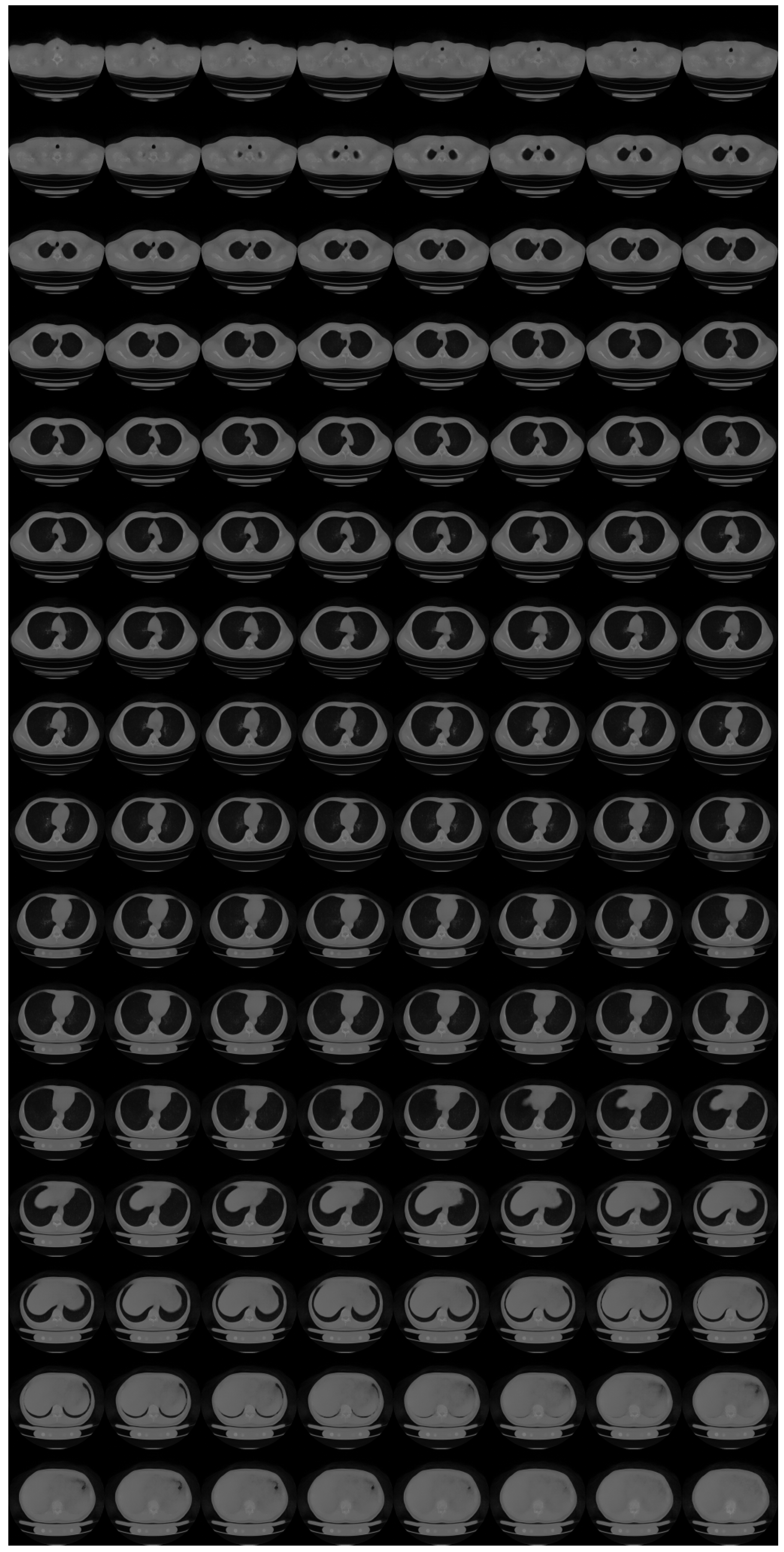
- We showcase a 3D flow-based deep generative model of 3D chest CT images, which has state-of-the-art resolution ().
2. Materials and Methods
2.1. Materials
2.2. Pre-Processing
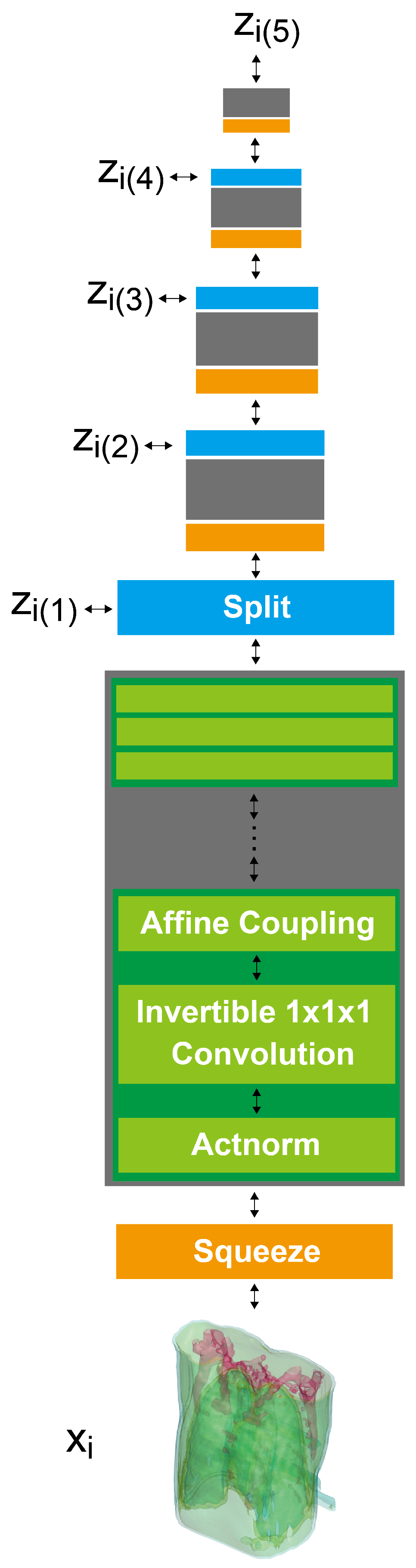
2.3. 3D GLOW
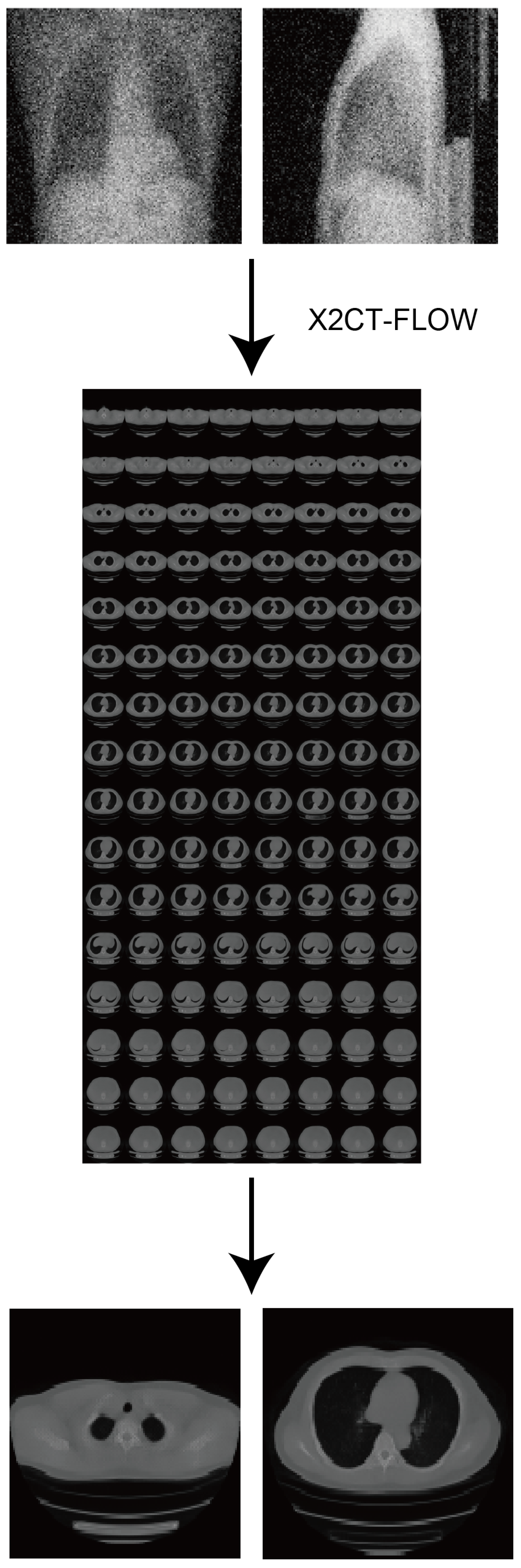
2.4. X2CT-FLOW
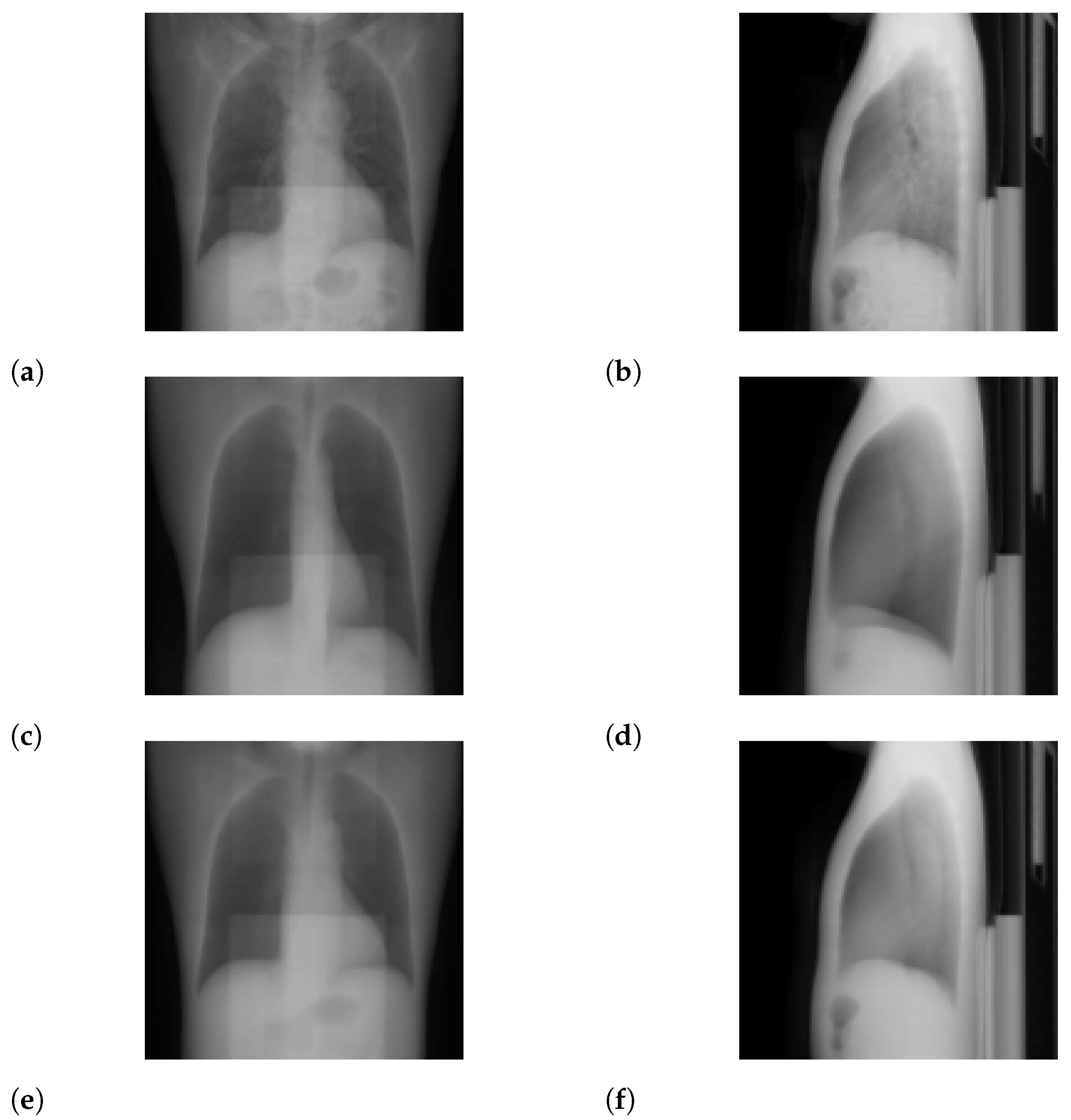
2.5. Validations
3. Results
3.1. Standard-Dose Protocol
3.2. Ultra-Low-Dose Protocol

4. Discussion
5. Conclusions
Author Contributions
Funding
Institutional Review Board Statement
Informed Consent Statement
Data Availability Statement
Acknowledgments
Conflicts of Interest
Abbreviations
| CT | computed tomography |
| MAP | maximum a posteriori |
| 2D | two-dimensional |
| 3D | three-dimensional |
| PSNR | peak signal-to-noise ratio |
| SSIM | structural similarity |
| MAE | mean absolute error |
| NRMSE | normalized root mean square error |
| CXR | chest X-ray |
Appendix A. Details for Progressive Learning
- import numpy as np
- # src : source image (ndarray)
- # n_bits_dst : the number of bits for the destination image
- # (integer)
- # n_bits_src : the number of bits for the source image
- # (integer)
- # return : destination image with reduction (ndarray)
- def color_reduction(src, n_bits_dst = 4, n_bits_src = 8):
- dst = np.copy(src)
- delta = 2∗∗n_bits_src // 2∗∗n_bits_dst
- for c in range(2∗∗n_bits_src // delta):
- inds = np.where((delta ∗ c <= src) \
- & (delta ∗ (c + 1) > src))
- dst[inds] = (2 ∗ delta ∗ c + delta ) // 2
- return dst
Appendix B. Ablation Study for Progressive Learning


Appendix C. Formulations for N ≥ 2
References
- Nam, J.G.; Ahn, C.; Choi, H.; Hong, W.; Park, J.; Kim, J.H.; Goo, J.M. Image quality of ultralow-dose chest CT using deep learning techniques: Potential superiority of vendor-agnostic post-processing over vendor-specific techniques. Eur. Radiol. 2021, 31, 5139–5147. [Google Scholar] [CrossRef]
- Levitan, E.; Herman, G.T. A maximum a posteriori probability expectation maximization algorithm for image reconstruction in emission tomography. IEEE Trans. Med. Imaging 1987, 6, 185–192. [Google Scholar] [CrossRef]
- Baraniuk, R.G. Compressive sensing [lecture notes]. IEEE Signal Process. Mag. 2007, 24, 118–121. [Google Scholar] [CrossRef]
- Shen, L.; Zhao, W.; Capaldi, D.; Pauly, J.; Xing, L. A Geometry-Informed Deep Learning Framework for Ultra-Sparse 3D Tomographic Image Reconstruction. arXiv 2021, arXiv:2105.11692. [Google Scholar] [CrossRef] [PubMed]
- Shen, L.; Zhao, W.; Xing, L. Patient-specific reconstruction of volumetric computed tomography images from a single projection view via deep learning. Nat. Biomed. Eng. 2019, 3, 880–888. [Google Scholar] [CrossRef] [PubMed]
- Ying, X.; Guo, H.; Ma, K.; Wu, J.; Weng, Z.; Zheng, Y. X2CT-GAN: Reconstructing CT from biplanar X-rays with generative adversarial networks. In Proceedings of the IEEE/CVF Conference on Computer Vision and Pattern Recognition, Long Beach, CA, USA, 15–20 June 2019; pp. 10619–10628. [Google Scholar]
- Peng, C.; Liao, H.; Wong, G.; Luo, J.; Zhou, S.K.; Chellappa, R. XraySyn: Realistic View Synthesis From a Single Radiograph Through CT Priors. arXiv 2020, arXiv:2012.02407. [Google Scholar]
- Henzler, P.; Rasche, V.; Ropinski, T.; Ritschel, T. Single-image Tomography: 3D Volumes from 2D Cranial X-Rays. In Computer Graphics Forum; Wiley Online Library: Hoboken, NJ, USA, 2018; Volume 37, pp. 377–388. [Google Scholar]
- Shibata, H.; Hanaoka, S.; Nomura, Y.; Nakao, T.; Sato, I.; Sato, D.; Hayashi, N.; Abe, O. Department of Radiology, The University of Tokyo Hospital, 7-3-1 Hongo, Bunkyo-ku, Tokyo, 113-8655, Japan. Search articles by ’Osamu Abe’ Abe O. Versatile anomaly detection method for medical images with semi-supervised flow-based generative models. Int. J. Comput. Assist. Radiol. Surg. 2021, 16, 2261–2267. [Google Scholar] [CrossRef] [PubMed]
- Kobyzev, I.; Prince, S.; Brubaker, M. Normalizing flows: An introduction and review of current methods. IEEE Trans. Pattern Anal. Mach. Intell. 2020, 43, 964–3979. [Google Scholar] [CrossRef] [PubMed]
- Kingma, D.P.; Dhariwal, P. Glow: Generative flow with invertible 1x1 convolutions. arXiv 2018, arXiv:1807.03039. [Google Scholar]
- Parmar, N.; Vaswani, A.; Uszkoreit, J.; Kaiser, L.; Shazeer, N.; Ku, A.; Tran, D. Image transformer. In Proceedings of the International Conference on Machine Learning, Stockholm, Sweden, 10–15 July 2018; pp. 4055–4064. [Google Scholar]
- Dinh, L.; Krueger, D.; Bengio, Y. Nice: Non-linear independent components estimation. arXiv 2014, arXiv:1410.8516. [Google Scholar]
- Dinh, L.; Sohl-Dickstein, J.; Bengio, S. Density estimation using real nvp. arXiv 2016, arXiv:1605.08803. [Google Scholar]
- Wang, Z.; Bovik, A.C.; Sheikh, H.R.; Simoncelli, E.P. Image quality assessment: From error visibility to structural similarity. IEEE Trans. Image Process. 2004, 13, 600–612. [Google Scholar] [CrossRef] [PubMed] [Green Version]
- Zeng, D.; Huang, J.; Bian, Z.; Niu, S.; Zhang, H.; Feng, Q.; Liang, Z.; Ma, J. A simple low-dose X-ray CT simulation from high-dose scan. IEEE Trans. Nucl. Sci. 2015, 62, 2226–2233. [Google Scholar] [CrossRef] [PubMed] [Green Version]
- Kothari, K.; Khorashadizadeh, A.; de Hoop, M.; Dokmanić, I. Trumpets: Injective Flows for Inference and Inverse Problems. arXiv 2021, arXiv:2102.10461. [Google Scholar]
- Asim, M.; Daniels, M.; Leong, O.; Ahmed, A.; Hand, P. Invertible generative models for inverse problems: Mitigating representation error and dataset bias. In Proceedings of the International Conference on Machine Learning, Virtual, 12–18 July 2020; pp. 399–409. [Google Scholar]
- Whang, J.; Lei, Q.; Dimakis, A.G. Compressed sensing with invertible generative models and dependent noise. arXiv 2020, arXiv:2003.08089. [Google Scholar]
- Whang, J.; Lindgren, E.; Dimakis, A. Composing Normalizing Flows for Inverse Problems. In Proceedings of the International Conference on Machine Learning, Virtual, 18–24 July 2021; pp. 11158–11169. [Google Scholar]
- Marinescu, R.V.; Moyer, D.; Golland, P. Bayesian Image Reconstruction using Deep Generative Models. arXiv 2020, arXiv:2012.04567. [Google Scholar]
- Menon, S.; Damian, A.; Hu, S.; Ravi, N.; Rudin, C. PULSE: Self-supervised photo upsampling via latent space exploration of generative models. In Proceedings of the IEEE/CVF Conference on Computer Vision and Pattern Recognition, Seattle, WA, USA, 13–19 June 2020; pp. 2437–2445. [Google Scholar]
- Ho, J.; Chen, X.; Srinivas, A.; Duan, Y.; Abbeel, P. Flow++: Improving flow-based generative models with variational dequantization and architecture design. In Proceedings of the International Conference on Machine Learning, Beach, CA, USA, 10–15 June 2019; pp. 2722–2730. [Google Scholar]
- Chen, R.T.; Behrmann, J.; Duvenaud, D.; Jacobsen, J.H. Residual flows for invertible generative modeling. arXiv 2019, arXiv:1906.02735. [Google Scholar]


| Flow coupling | Affine |
| Learn-top option | True |
| Flow permutation | 1 × 1 × 1 convolution |
| Minibatch size | 1 per GPU |
| Train epochs | 96 (2 bits) |
| 324 (3 bits from 2 bits) | |
| 24 (4 bits from 3 bits) | |
| 144 (8 bits from 4 bits) | |
| Layer levels | 5 |
| Depth per level | 8 |
| Filter width | 512 |
| Learning rate in steady state |
| Method | Ours | X2CT-GAN [6] |
| SSIM | 0.4897 (0.00437) | 0.5349 (0.001257) |
| PSNR [dB] | 17.57 (4.755) | 19.53 (1.152) |
| MAE | 0.08299 (0.001008) | 0.005758 (6.17 × 10) |
| NRMSE | 0.1374 (0.002066) | 0.1064 (0.0001714) |
| Method | Ours | X2CT-GAN [6] |
| SSIM | 0.7675 (0.001931) | 0.7543 (0.0005110 ) |
| PSNR [dB] | 25.89 (2.647) | 25.22 (0.5241) |
| MAE | 0.02364 () | 0.02648 (5.552 × 10⁻⁶) |
| NRMSE | 0.05731 (0.0002204) | 0.05502 (2.181 × 10⁻⁵) |
| Method | Ours | X2CT-GAN [6] |
| SSIM | 0.4989 (0.000536) | 0.5151 (0.001028) |
| PSNR (dB) | 18.16 (0.1560) | 19.38 (0.9493) |
| MAE | 0.07480 (2.98 × 10⁻⁵) | 0.005943 () |
| NRMSE | 0.1237 (3.20 × 10⁻⁵) | 0.1081 () |
| Method | Ours | X2CT-GAN [6] |
| SSIM | 0.7008 (0.0005670) | 0.6828 (0.0002700) |
| PSNR (dB) | 23.58 (0.6132) | 23.78 (0.2827) |
| MAE | 0.02991 () | 0.03251 (4.193 × 10⁻⁶) |
| NRMSE | 0.07349 () | 0.06486 (1.607 × 10⁻⁵) |
Publisher’s Note: MDPI stays neutral with regard to jurisdictional claims in published maps and institutional affiliations. |
© 2022 by the authors. Licensee MDPI, Basel, Switzerland. This article is an open access article distributed under the terms and conditions of the Creative Commons Attribution (CC BY) license (https://creativecommons.org/licenses/by/4.0/).
Share and Cite
Shibata, H.; Hanaoka, S.; Nomura, Y.; Nakao, T.; Takenaga, T.; Hayashi, N.; Abe, O. On the Simulation of Ultra-Sparse-View and Ultra-Low-Dose Computed Tomography with Maximum a Posteriori Reconstruction Using a Progressive Flow-Based Deep Generative Model. Tomography 2022, 8, 2129-2152. https://doi.org/10.3390/tomography8050179
Shibata H, Hanaoka S, Nomura Y, Nakao T, Takenaga T, Hayashi N, Abe O. On the Simulation of Ultra-Sparse-View and Ultra-Low-Dose Computed Tomography with Maximum a Posteriori Reconstruction Using a Progressive Flow-Based Deep Generative Model. Tomography. 2022; 8(5):2129-2152. https://doi.org/10.3390/tomography8050179
Chicago/Turabian StyleShibata, Hisaichi, Shouhei Hanaoka, Yukihiro Nomura, Takahiro Nakao, Tomomi Takenaga, Naoto Hayashi, and Osamu Abe. 2022. "On the Simulation of Ultra-Sparse-View and Ultra-Low-Dose Computed Tomography with Maximum a Posteriori Reconstruction Using a Progressive Flow-Based Deep Generative Model" Tomography 8, no. 5: 2129-2152. https://doi.org/10.3390/tomography8050179