Improved Networks Routing Using an Arrow-Based Description

Abstract

In this paper, an improved routing algorithm suitable for planar networks—static Zigbee and mesh networks included—is shown. The algorithm is based on the cycle description of the graph, and on a new graph model based on arrow description, which is outlined. We show that the newly developed model allows for a faster algorithm for finding a direct and a return path in the network. The newly developed model allows further interpretations of the relationships in any simple planar graphs. Examples showing the implementation of the newly developed model are presented too.

1. Introduction

This paper is the extended version of the reference [1] presented at MOCAST 2020 conference. The routing algorithm and its extension is suitable for static ZigBee and mesh networks [2,3,4,5].

Many types of networks deployed for every-day use including home networks, static sensor networks, etc. can be modeled as a connected planar graph, described using either its node or its cycle description.

The networks are cyclically connected such that a cycle description of the associated graph is possible.

Routing is an essential feature of any communication network. Almost any networks-related standard, including those by IEEE Zigbee IEEE 802.15.4, recommends the existence of routing protocols. The cornerstone of routing is the ability to find paths between two given end nodes. Most of such algorithms rely on node hopping and are based on the node description of the graph associated to the network [2,3,4,5]. We note that many types of networks deployed in everyday use (including home networks, static sensor networks, etc.) can be modeled as a connected planar graph.

In a previous paper [6], it has been shown that a routing algorithm can be developed using the cycle description of the underlying graph. This method has several advantages over algorithms based on node-hopping, such as its lack of back-tracking.

However, one disadvantage of the method presented in [6] was that the data obtained as the result of the algorithm are difficult to process. In this paper, we address this shortcoming by means of a new “arrows” model for the graph. This model significantly improves the path-finding algorithm based on cycles mergers.

The paper is organized as follows:

• Section 2 introduces the basic notations used in the paper;
• Section 3 describes an arrow-description of the graph;
• Section 4 describes the use of the arrow algebra;
• Section 5 describes the routing algorithm using arrows;
• Section 6 is dedicated to a more detailed description of the algorithm;
• Section 7 is dedicated to conclusions and future work.

2. Basic Definitions and Notations

2.1. Background

It is known that any graph is represented by a set of links, which are connected to each other via nodes [7]. The number of links departing or arriving in a node is called the degree of the node. A link connected to a node is said to be incident to the node. A suite of links connecting two end nodes by passing through other nodes is called a path. A closed path, i.e., a path starting and ending in the same node is called a cycle. A cycle that visits every node of the graph exactly once is called a Hamiltonian cycle; a graph that has at least one Hamiltonian cycle is called a Hamiltonian graph. A link connected to a cycle, i.e., a component of a given cycle, is said to be incident to the cycle. Two cycles are adjacent if they share only a single link.

The total number of nodes in the graph is denoted as N and the number of links is denoted as L. In this paper, we use simple planar connected graphs, which have no self-looping nodes, no leaves (nodes of degree 1) and no parallel links between any two nodes.

Algebraically, the graph’s connectivity can be described by using either the nodes–links or the cycles–links incidence matrix. The nodes–links incidence matrix A is an N×L matrix (it has N rows and L columns), whose elements describe which links connect which nodes. The cycles–links incidence matrix B is a C×L matrix, where C is the number of independent cycles, and L, the number of links of the graph. In a planar graph, the values C, L, and N are such that [8] they fulfill the Euler equation C = L-N + 2.

Labeling is used to uniquely identify different parts of the graph, such as nodes, links, and cycles. In addition, graphs representing nodes are usually undirected. However, a randomly chosen direction is used in order to, e.g., analyze network functions. Neither the chosen labeling, nor the added direction, directly influence the properties of the graph.

In a planar graph, its cycles divide the geometric plane into an internal and an external region, and a cycle defines the border between the two regions. In this paper, we index the cycles such that the set of the cycles C is defined as C = {C1, C2, …, C_c} and we assume that the cycle with the highest index C_c is the border cycle, and c is given by the Euler equation. Recall that a planar graph is a graph that can be drawn in a planar embedding such that no link crossings are present.

We present the cycles description of a graph subsequently. This description can be adopted for any simple, planar, cyclically connected graph [1].

In this paper, we will use an incidence matrix describing how the links are related to the cycles. This matrix is the cycles–links incidence matrix B_CxL of the associated graph, which will be presented in a later paragraph. It is orthogonal to the nodes–links incidence matrix A. [7,8].

2.2. Adjacency and Cycles Merger

Onete and Onete defined [7,9] the notion of cycle merger, which is applicable to adjacent cycles only. We only briefly describe this notion below, as it was already described in [5].

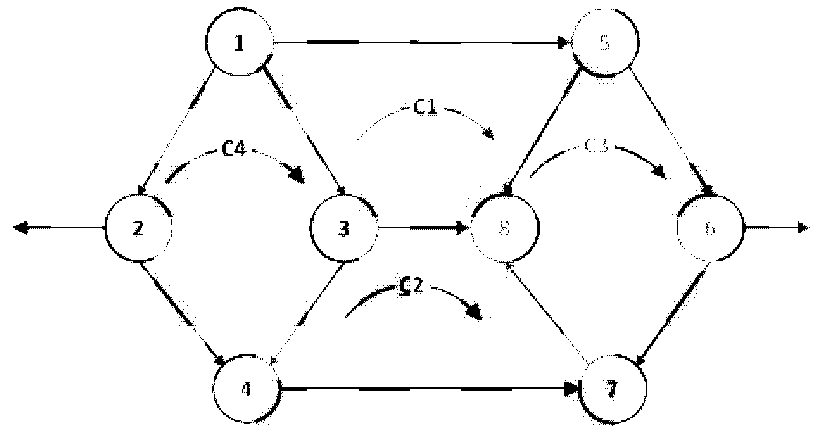
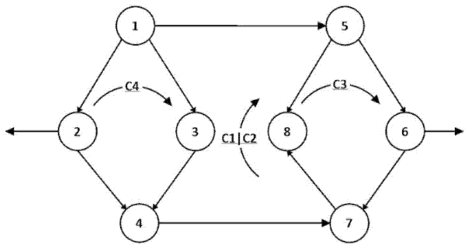
Figure 1 depicts a subnetwork in which the nodes and the cycles are labeled, and a direction was defined for the links and cycles as previously discussed. Note that for example cycles c₁ and c₂ are adjacent through the common link connecting nodes 3 and 8. The two cycles can be merged as shown in Figure 2, following the method of [7,9]. Notably, we obtain a larger cycle by removing the adjacent link of the two cycles. Algebraically this can be obtained by adding either the rows or the columns describing c₁ and c₂ in the matrix L_C, as described by [7]. Notably, L_C is the cycles Laplacian of the network and it is obtained using the cycles–links incidence matrix: L_C = B*B^T.

We depict the result of the merger, denoted c₁|c₂ in Figure 2.

The authors of two papers [9,10] describe an algorithm of obtaining the Hamiltonian cycles in a graph by using cycle merger. This method needs no backtracking and thus the algorithm is parallelizable.

3. An Arrow-Based Description and Its Algebra

3.1. Graph Arrows

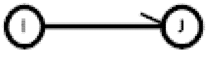
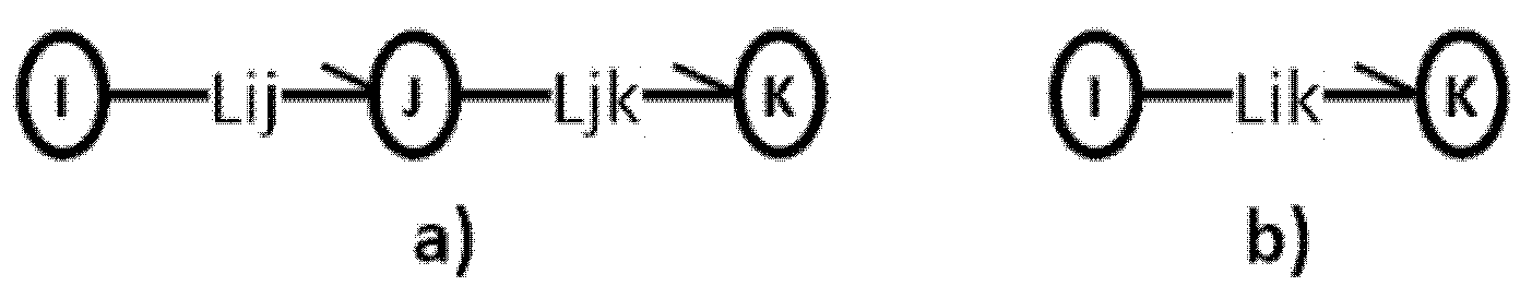
In this section we define graph arrows as an algebraic object, then proceed to describe operations on such objects. We depart from a (finite) set of nodes N. We define an arrow as an ordered tuple $\overrightarrow{\left(I, J\right)}$ with $I, J\in N$. Intuitively, this object will correspond to a directed arrow from node I to node J, as depicted in Figure 3:

In addition to arrows of the form $\overrightarrow{\left(i, j\right)}$, we define two special types of arrows. The first is called the zero arrow $\overrightarrow{0}$, defined as an arrow from any node to itself. Thus, $\overrightarrow{\left(i,i\right)}=\overrightarrow{\left(j,j\right)}= \overrightarrow{0}$. This special zero arrow is in fact an equivalence class of self-loops. The second is the neutral arrow, denoted $\overrightarrow{\infty }$.

We define an “addition” operation on graph arrows, which we denote as $\overrightarrow{+}$.

Definition 1.

Let$N$be a node set and let$i,j, k, l\in N$be nodes in that node set. Let$\overrightarrow{\infty }$and$\overrightarrow{0}$be the two special nodes defined above. We define the addition operation$\overrightarrow{+}$as follows:

• $\overrightarrow{\left(i,j\right)} + \overrightarrow{\left(j,k\right)}= \overrightarrow{\left(i,k\right)}$;
• $\overrightarrow{\left(i,j\right)} + \overrightarrow{\left(i,j\right)}= \overrightarrow{\left(i,j\right)}$;
• $\overrightarrow{\left(i,j\right)} + \overrightarrow{\left(k,i\right)}= \overrightarrow{\left(k,j\right)}$; $\overrightarrow{\left(i,j\right)} + \overrightarrow{\left(k,l\right)}= \overrightarrow{\infty }$ if $i\ne l$ and $j\ne k$;
• $\overrightarrow{\left(i,j\right)} + \overrightarrow{0}= \overrightarrow{0} + \overrightarrow{\left(i, j\right)}=\overrightarrow{\left(i, j\right)}$;
• $\overrightarrow{\infty }+ \overrightarrow{\left(i, j\right)}= \overrightarrow{\left(i, j\right)}+ \overrightarrow{\infty }= \overrightarrow{\infty }$;
• $\overrightarrow{0}+ \overrightarrow{\infty }= \overrightarrow{\infty }+ \overrightarrow{0}= \overrightarrow{\infty }$.
• $\overrightarrow{0}+ \overrightarrow{0}= \overrightarrow{0}$

Consider the set of arrows defined by $\left(N x N\right){{\displaystyle \cup }}^{} \overrightarrow{0}{{\displaystyle \cup }}^{} \overrightarrow{\infty }$ under the operation of arrow addition +. This structure is closed under addition, it has an identity element $\overrightarrow{0}$, and it is commutative. Moreover, using the first rule it holds that $\overrightarrow{\left(i, j\right)} + \overrightarrow{\left(j, i\right)}= \overrightarrow{\left(i, i\right)}= \overrightarrow{0}$. As a result, we usually call $\overrightarrow{\left(j,i\right)}$ the inverse of $\overrightarrow{\left(i, j\right)}$. Note that for each arrow of the form $\overrightarrow{\left(i, j\right)}$ there is a unique inverse. The inverse of $\overrightarrow{0}$ is itself. However, the neutral element has no inverse. In addition, the addition operation we have defined is not generally associative. Indeed, it holds that:

$$\left[\overrightarrow{\left(i,j\right)} \overrightarrow{+} \overrightarrow{\left(k,l\right)}\right]+ \overrightarrow{\left(j,k\right)}= \overrightarrow{\infty }+ \overrightarrow{\left(j, k\right)}= \overrightarrow{\infty }$$

However, associating the second and third terms yields a different result:

$$\overrightarrow{\left(i,j\right)}+ \left[\overrightarrow{\left(k,l\right)} + \overrightarrow{\left(j,k\right)}\right] = \overrightarrow{\left(i,j\right)}+ \overrightarrow{\left(j, l\right)}= \overrightarrow{\left(i,l\right)}$$

The operation of inverting a graph arrow is shown in Figure 4, where the inverse of the full arrow is the dotted one.

3.2. Basic Graph Operations with Arrows

Our goal is to ultimately express cycle merger in terms of arrow addition. We first draw a parallel between planar graphs, their nodes and links, and our graph arrow structure. We view the node at infinity as a single node, defined more particularly by the addition that created it. We will additionally view links in the graph as a tuple of arrows, one direct, and one inverse, between the nodes—this will be shown in Section 4.

4. Using Graph Arrows

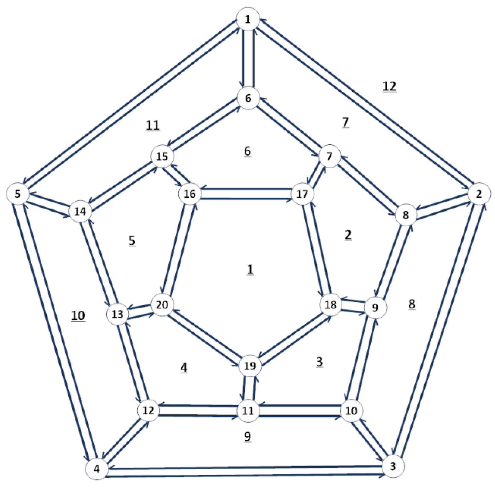
In this section, we show how to use graph arrow addition in finding Hamiltonian circuits, by using as an example the figure of the dodecahedron shown in Figure 5. Typically, a dodecahedron has single links between the nodes; however, our first step is to de-duplicate each link into two graph arrows, one direct and one inverse.

We label the cycles of the dodecahedron in underlined numbers and choose a random orientation for each cycle (clockwise for the inside cycles, counterclockwise for the outside one). Adjacent cycles, such as 11 and 6, have one link in common; however, this link is traveled in one direction in one cycle, and in the opposite direction in the adjacent one. As we will indeed show, when de-duplicating the links into graph arrows, this allows us to associate the direct graph arrow to one cycle, and its inverse, to the other. In

Table 1. Cycles–arrows description. Reprinted with permission from [1].

Cycle	Arrows
1	$\overrightarrow{\left(16,17\right)}$,$\overrightarrow{\left(17,18\right)}$,$\overrightarrow{\left(18,19\right)}$,$\overrightarrow{\left(19,20\right)}$,$\overrightarrow{\left(20,16\right)}$
2	$\overrightarrow{\left(18,17\right)}$,$\overrightarrow{\left(17,7\right)}$,$\overrightarrow{\left(7,8\right)}$,$\overrightarrow{\left(8,9\right)}$,$\overrightarrow{\left(9,18\right)}$
3	$\overrightarrow{\left(18,9\right)}$,$\overrightarrow{\left(9,10\right)}$,$\overrightarrow{\left(10,11\right)}$,$\overrightarrow{\left(11,19\right)}$,$\overrightarrow{\left(19,18\right)}$
4	$\overrightarrow{\left(19,11\right)}$,$\overrightarrow{\left(11,12\right)}$,$\overrightarrow{\left(12,13\right)}$,$\overrightarrow{\left(13,20\right)}$,$\overrightarrow{\left(20,19\right)}$
5	$\overrightarrow{\left(20,13\right)}$,$\overrightarrow{\left(13,14\right)}$,$\overrightarrow{\left(14,15\right)}$,$\overrightarrow{\left(15,16\right)}$,$\overrightarrow{\left(16,20\right)}$
6	$\overrightarrow{\left(15,6\right)}$,$\overrightarrow{\left(6,7\right)}$,$\overrightarrow{\left(7,17\right)}$,$\overrightarrow{\left(17,16\right)}$,$\overrightarrow{\left(16,15\right)}$
7	$\overrightarrow{\left(1,2\right)}$,$\overrightarrow{\left(2,8\right)}$,$\overrightarrow{\left(8,7\right)}$,$\overrightarrow{\left(7,6\right)}$,$\overrightarrow{\left(6,1\right)}$
8	$\overrightarrow{\left(2,3\right)}$,$\overrightarrow{\left(3,10\right)}$,$\overrightarrow{\left(10,9\right)}$,$\overrightarrow{\left(9,8\right)}$,$\overrightarrow{\left(8,2\right)}$
9	$\overrightarrow{\left(3,4\right)}$,$\overrightarrow{\left(4,12\right)}$,$\overrightarrow{\left(12,11\right)}$,$\overrightarrow{\left(11,10\right)}$,$\overrightarrow{\left(10,3\right)}$
10	$\overrightarrow{\left(4,5\right)}$,$\overrightarrow{\left(5,14\right)}$,$\overrightarrow{\left(14,13\right)}$,$\overrightarrow{\left(13,12\right)}$,$\overrightarrow{\left(12,4\right)}$
11	$\overrightarrow{\left(5,1\right)}$,$\overrightarrow{\left(1,6\right)}$,$\overrightarrow{\left(6,15\right)}$,$\overrightarrow{\left(15,14\right)}$,$\overrightarrow{\left(14,5\right)}$
12	$\overrightarrow{\left(1,5\right)}$,$\overrightarrow{\left(5,4\right)}$,$\overrightarrow{\left(4,3\right)}$,$\overrightarrow{\left(3,2\right)}$,$\overrightarrow{\left(2,1\right)}$

, we present the graph-arrow description of the cycles, in which we have deduplicated the links into two arrows which are inverse to one another. This table shows the correspondence between nodes and cycles, and can furthermore be used to generate the cycles–links incidence matrix B.

For the case of the dodecahedron, this incidence matrix has 30 entries per row (the number of links) and will be not be represented here because of a lack of space. However, the non-zero entries, corresponding to the links found in each cycle, are found in Table 1. As the nodes–links and cycles–links incidence matrices are orthogonal, there is no direct adjacency matrix between the nodes and cycles of a graph. However, we can use matrix B to find paths in the graph, as we shall show subsequently.

5. Routing Algorithm Using Arrows

As discussed in Section 1, our graph-arrow addition method will be applied to a specific path-finding algorithm, namely one based on cycle–merger.

In this method, in order to find a route between an initial node $i$ and a final node $f$, we must first identify which cycles comprise those nodes. Recall that if a node has a degree d then the respective node can be found in d cycles [7]. Once all such cycles have been identified, one creates a Laplacian of the cycles, and we perform the cycle–merger algorithm until the two nodes are within the same larger cycle [9,10,11]. At this moment we know which cycles have participated in a merger. Furthermore, because the result of the program is a larger cycle, a direct path and a return paths exist. The program can be extended to provide all possible routing paths connecting the starting node and the final node, but this will be more time consuming.

The next step should be identifying the routing paths. The result of the algorithm of [6] was a list of the traveled cycles. The complexity of translating this list to usable routes was not taken into account for the complexity analysis and is indeed costly. In the following, we will optimize the format of the results towards a possible use in routing.

Suppose that in our example of the dodecahedron we want to find a path between the start node $i=1$ and the final node $f=20$. In the original paper, cycle merger is done starting from rows of the cycle–links incidence matrix. We do the same here, but we depart from the cycle–arrow incidence matrices. Each time we are meant to merge two cycles, we add the corresponding rows by using the rules of the addition operation described in Definition 1.

Following the algorithm ultimately results in (for instance) the following vector for which non-zero entries are given in Equation (1).

$$\begin{array}{l}[\overrightarrow{\left(\mathbf{5},\mathbf{1}\right)}, \overrightarrow{\left(\mathbf{1},\mathbf{2}\right)}, \overrightarrow{\left(\mathbf{3},\mathbf{4}\right)},\overrightarrow{\left(\mathbf{6},\mathbf{15}\right)}, \overrightarrow{\left(\mathbf{7},\mathbf{6}\right)}, \overrightarrow{\left(\mathbf{8},\mathbf{9}\right)}, \overrightarrow{\left(\mathbf{9},\mathbf{19}\right)}, \overrightarrow{\left(\mathbf{10},\mathbf{3}\right)},\overrightarrow{\left(\mathbf{13},\mathbf{20}\right)},\overrightarrow{\left(\mathbf{14},\mathbf{5}\right)}, \\ \overrightarrow{\left(\mathbf{2},\mathbf{8}\right)}, \overrightarrow{\left(\mathbf{12},\mathbf{13}\right)}, \overrightarrow{\left(\mathbf{4},\mathbf{12}\right)},\overrightarrow{\left(\mathbf{14},\mathbf{5}\right)},\overrightarrow{\left(\mathbf{18},\mathbf{19}\right)},\overrightarrow{\left(\mathbf{11},\mathbf{10}\right)},\overrightarrow{\left(\mathbf{20},\mathbf{16}\right)},\overrightarrow{\left(\mathbf{16},\mathbf{17}\right)}, \overrightarrow{\left(\mathbf{17},\mathbf{7}\right)}, \overrightarrow{\left(\mathbf{19},\mathbf{11}\right)}\end{array}$$

(1)

We note that each entry of this vector represents a tuple of values, each in the set of nodes N. As a first step, we create two node lists: a list denoted $T$ which will contain the first nodes (tails) of each arrow, and a list denoted $H$ which will contain the second nodes (heads) of each arrow. Our goal is to find a path between our chosen nodes, 1 and 20.

We first apply the Knuth–Morris–Pratt (KMP) algorithm [12] to the tail list $T$ to find node 1. Subsequently we find the node that is at the same index in the head list $H$ as the node 1 was in the list $T$; denote this node by $j$. We now remove node $i$ from list $T$ and $j$ from $H$. We subsequently search for node $j$ in list $T$ (using the KMP algorithm), and then continue in the same way until we reach node $f$. This will give us a path from $i$ to $f$.

For our example, we start from node 1 in list $T$: we find it on the second position. To this corresponds the value $2$ in list $H$. We remove the two values and continue. We find node $2$ in $T$ and the corresponding value is node $10$ in list $H$, etc.

The following operations involving the arrows can be defined and described.

5.1. Serial Addition

Consider a graph containing the nodes $i,j,k$ shown in Figure 6a, linked by graph arrows (representing directed links in the graph). The addition operation yields the arrow in Figure 6b.

5.2. Parallel Composition of Graph Arrows

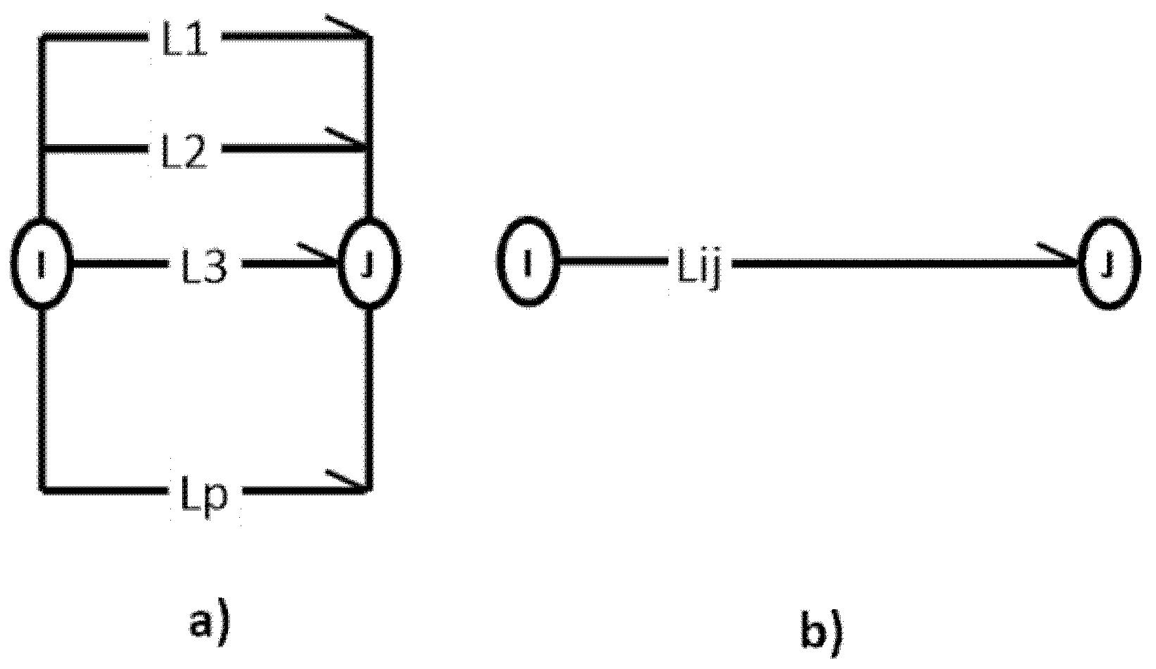
For the most part, in this paper, we have considered graphs which contain no parallel links. However, the arrow addition operation may yield such parallel links. The second rule of addition shows us that the parallel composition of graph arrows as depicted in Figure 7a yields a single arrow as shown in Figure 7b.

5.3. Series-Parallel Composition of Graph Arrows

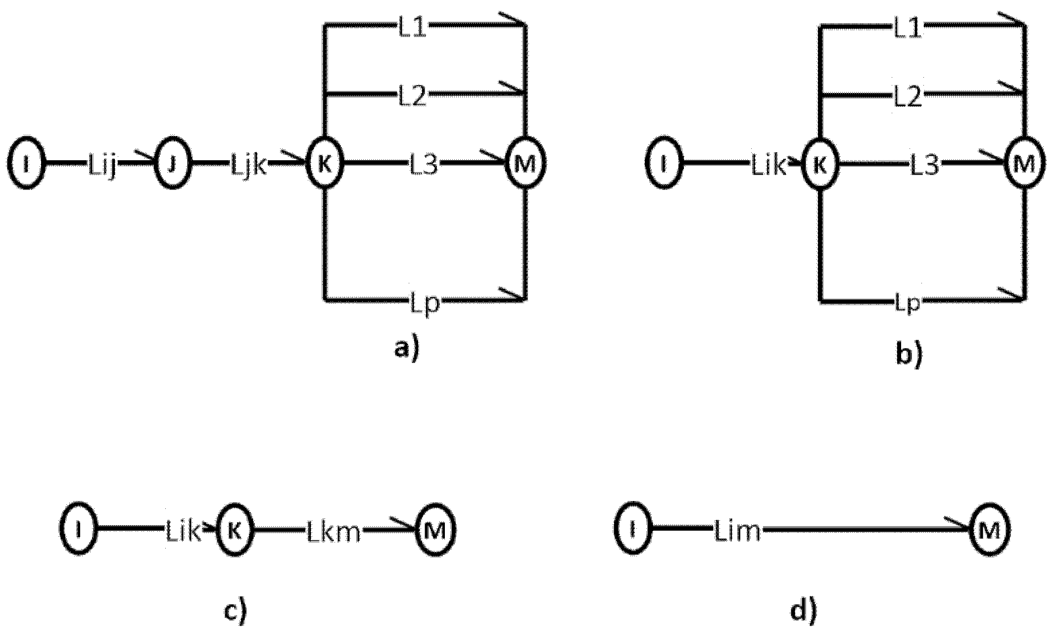
We can combine the two basic operations we described in the previous sections.

We begin from the complex graph in Figure 8a. By a serial composition on the first three nodes we would obtain the graph in Figure 8b. The parallel composition of the arrows in the right-most node yields Figure 8c. Finally, a renewed serial composition yields the arrow in Figure 8d.

We note that using a sequence of serial and parallel compositions based on arrow addition will ultimately turn a complex planar graph into a simple one, as it will eliminate self-loops and parallel links.

The following Algorithm 1 describes the path finding using graph arrows:

Algorithm 1: The path finding using graph arrows.

Input: the starting node nsand the end node ne;     Determine the cycles containing nsand ne;     Determine the cycles paths comprising both nsand ne       using cycles mergers;     If there is no path, then STOP and print “No path found”;     Once a path is found, translate the list of graph arrows        to sets T and H as discussed.     By successive applications of the KMP algorithm as        described above, find a direct and a return path        between the nodes;  Output: the path discovered.

The following observations apply (see [6]):

• Each time, the number of cycles limits the iterations to less than C.
• The end criteria of the program can be flexible such that it can be stopped whenever a first path is found or alternatively it can be run until a path with a specific length is obtained.

Because of the linear costs of the KMP algorithm, the overall cost of finding the longest path becomes $O\left(N^2\right)$—the algorithm has linear complexity and it must be run at most $N$ times. Obviously, the additional finding that the Knuth–Morris–Pratt algorithm adds nothing to the complexity encourages us to say that there are good prospects that the algorithm may be used in real-time systems.

Dijkstra’s algorithm [13,14] describes how to find a path between a source node and an end node in a given graph. Its complexity depends on graph sparsity and on data representation and in the most optimistic case its complexity is O(N). This algorithm, however, only finds the shortest path in a graph, yielding thus the same result consistently if the graph, the source, and the end nodes are unchanged. This does not, therefore, take into account particularities of the telecom network, which requires redundant paths to avoid collisions and congested traffic. If run on all the nodes, Dijkstra’s algorithm has a worst-case complexity of O(N²), as with the algorithm presented in this paper.

Incidentally, let us observe that the Algorithm 1 presented in this paper also provides for a return path which is different that the direct path and therefore any collision that may occur can be avoided.

6. The Algorithm in More Detail

Initially, we run the first part of the algorithm as indicated in [5] and find the necessary cycles adjacencies that would determine a direct and a reverse path in the graph from a given source node to an end node. To do that, we first randomly number the nodes of the graph. Then we choose a parsing direction for each cycle. Usually, we use the same parsing direction for each internal cycle and the opposite direction for the border cycle. In our example, we have chosen the clockwise direction for the internal cycle and the counterclockwise direction for the external cycle.

Afterwards we assign arrows to each link such that the arrows belonging to a specific cycle have the same orientation as the orientation of the cycle. These assignments are depicted in Figure 5.

Furthermore, we randomly number the links in the graph such that they are uniquely identified. Recall that a link is shown as a composition of two arrows, running in opposite directions. In Figure 5, the link numbers are not shown for the sake of clarity.

Once we have made these preliminary assignments, we can create the cycles Laplacian of the graph, which is used in finding a direct path and a reverse path in the graph as it is shown in the literature [6,9,10].

In parallel, we need to have a representation of the dependencies between the cycles and the nodes. However, a purely numerical dependency does not exist because the nodes–links incidence matrix A_nxL is orthogonal to the cycles–links incidence matrix B_CxL and therefore AB = BA = 0, wherein 0 in a matrix with all the entries equaling 0. Hence, a symbolic representation of nodes–cycles dependencies looks appropriate, as well as a list-based one. In this paper, we prefer the symbolic representation and we show it subsequently.

For this purpose, we need to use the arrow representation of the graph together with all its properties as presented above.

For this purpose, each non-zero entry (i,j) in the cycles–links matrix is replaced by the arrow corresponding to the sense in which the link is traversed within that cycle.

In this way we have introduced the cycles–nodes dependencies. For example, the row in the matrix B corresponding to cycle 1 contains the non-zero entries in the second row of

Table 2. Links in cycle 1 in arrow notation.

26	27	28	29	30
$\overrightarrow{\left(19,20\right)}$	$\overrightarrow{\left(20,16\right)}$	$\overrightarrow{\left(16,17\right)}$	$\overrightarrow{\left(17,18\right)}$	$\overrightarrow{\left(18,19\right)}$

. The remaining entries on that row are zeroes and not shown below.

The first row of Table 2 indicates the link numbers assigned to the links of the graph shown in Figure 5. We note that link 27 contains node 20, which is the end node of the sought path.

Notice that cycles C1 and C2 are adjacent, with common link 29. As we already know from previous work [6], merging C1|C2 results in adding the corresponding rows or columns of the cycles Laplacian. We translate this operation using the cycle–nodes dependency for cycle1 and for cycle2, respectively and using the arrow representation. The result of the arrow operation related to link 29, which is the common link between cycles 1 and 2 is shown in Equation (2).

$$\overrightarrow{\left(\mathbf{17},\mathbf{18}\right)} \overrightarrow{+} \overrightarrow{\left(\mathbf{18},\mathbf{17}\right)}= \overrightarrow{\mathit{0}}$$

(2)

In Equation (2), we have used the fact that each link has an inverse.

At the end of the process we obtain the final cycle–links dependency vector of the merged cycle, whose non-zero entries are, in arrow notation, ($\overrightarrow{\left(\mathbf{19},\mathbf{20}\right)}, \overrightarrow{\left(\mathbf{20},\mathbf{16}\right)}$,$\overrightarrow{\left(\mathbf{16},\mathbf{17}\right)}, \overrightarrow{\left(\mathbf{17},\mathbf{7}\right)}, \overrightarrow{\left(\mathbf{7},\mathbf{8}\right)}$, $\overrightarrow{\left(\mathbf{8},\mathbf{9}\right)}, \overrightarrow{\left(\mathbf{9},\mathbf{18}\right)}, \overrightarrow{\left(\mathbf{18},\mathbf{19}\right)}$)

The next step in the algorithm is to separate the source and end nodes for each arrow. For the above merger, the vectors appear as in

Table 3. Source and end nodes for C1|C2 merger.

Arrow	Source	End
$\overrightarrow{\left(\mathbf{19},\mathbf{20}\right)}$	19	20
$\overrightarrow{\left(\mathbf{20},\mathbf{16}\right)}$	20	16
$\overrightarrow{\left(\mathbf{16},\mathbf{17}\right)}$	16	17
$\overrightarrow{\left(\mathbf{17},\mathbf{7}\right)}$	17	7
$\overrightarrow{\left(\mathbf{7},\mathbf{8}\right)}$	7	8
$\overrightarrow{\left(\mathbf{8},\mathbf{9}\right)}$	8	9
$\overrightarrow{\left(\mathbf{9},\mathbf{18}\right)}$	9	18
$\overrightarrow{\left(\mathbf{18},\mathbf{19}\right)}$	18	19

.

Now we apply the KMP algorithm in the following way. We look at the line 1 in the “Source” column and detect the corresponding element in the “End” column. Hence, we determine that node 19 is connected to node 20. We switch again to vector “From” looking now for From (20), which is element 2 in the vector, and then we find its corresponding element in the “To” vector as node 16.

The process is applied mutatis-mutandis until all the elements from both vectors are addressed. At the end of the process, the parsing nodes are revealed and a direct and a reverse path are both found.

As a general observation, the columns “Source” and “End” are easily generated from one single parsing of the final cycle obtained from the merger of any other cycles in the graph.

Equation (1) gives a direct and a return path from node 1 to node 20 and the resulting graph is depicted in Figure 9.

It is obtained running Algorithm 1 [5]. We have chosen the starting cycle C11 and afterwards we have performed the mergers C11|C7|C2|C1|C4|C9. Let us observe that we can obtain the same resulting graph if we start with cycle 12 and then we perform the mergers C12|C8|C3|C10|C5|C6.

Equation (1) gives a direct and return path from node 1 to node 20 in the graph in Figure 8. This can be viewed from the Source/End node table below (

Table 4. The direct and return path from node 1 to node 20.

Source	1	2	3	4	5	6	7	8	9	10	11	12	13	14	15	16	17	18	19	20
End	2	8	4	12	1	15	6	9	18	3	10	13	20	5	14	17	7	19	11	16

)

We can “read” the direct and return paths from this table by tracing consecutive links (links for which the source node of the second link is the end node of the first one). The resulting path from node 1 to node 20 is either like (1,2,8,9,19,11,10,3,4,12,13,20) or like (20,16,17,7,6,15,14,5,1). Each path could be direct or return because they both can be parsed either from left to right or in reverse order.

Furthermore, if we analyze the paths, we may choose the shortest one because the first one has 11 hops while the second one has only 8.

7. Conclusions and Further Work

In this paper, we have presented an alternative method to processing the results of the routing algorithm of [6].

A new graph model has been introduced based on graph-arrows, which in turn provides us with a very efficient implementation of the algorithm. It allows the use of Knuth–Morris–Pratt algorithm, which in turn provides limited overhead in execution time. This encourages us to use this approach in other problems related to graphs.

It is our belief that an arrow-based description of the graph is a very powerful tool for describing graphs and it is worthwhile using it in other graph-related problems.

So far, this is the only graph model that brings under the same concept all the elements of a graph: nodes, links and cycles.

References

- Onete, C.E.; Onete, M.C.C. Improved networks routing using link addition. In Proceedings of the MOCAST 2020, Bremen, Germany, 7–9 September 2020. [Google Scholar]
- Bhondekar, A.P.; Kaur, H. Routing Protocols in Zigbee Based Networks: A Survey. Available online: https://www.researchgate.net/publication/275637579 (accessed on 10 November 2019).
- Narmada, A.; Rao, P.S. Performance comparison of routing protocols for zigbee wpan. Int. J. Comput. Sci. Issues (IJCSI) 2011, 8, 394–402. [Google Scholar]
- Prativa, P.; Saraswala, A. Survey on routing protocols in zigbee network. Int. J. Eng. Sci. Innov. Technol. IJESIT 2013, 2, 471–476. [Google Scholar]
- Kumar, P.S.S.; Babu, A.R. A survey on routing techniques in zigbee wireless networks in contrast with other wireless networks. Indian J. Sci. Technol. 2017, 10, 1–8. [Google Scholar] [CrossRef]
- Onete, C.E.; Onete, M.C.C. An alternative to zigbee routing using a cycles description of a planar graph. In Proceedings of the 2019 8th International Conference on Modern Circuits and Systems Technologies (MOCAST), Thessaloniki, Greece, 13–15 May 2019; pp. 29–32. [Google Scholar]
- Bondy, A.; Murty, U.S.R. Graph Theory, Springer Graduate Texts in Mathematics; Springer: Berlin, Germany, 2008. [Google Scholar] [CrossRef]
- Balabanian, N.; Bickart, T.A. Electrical Network Theory; John Wiley and Sons Inc.: New York, NY, USA, 1969. [Google Scholar]
- Onete, C.E.; Onete, M.C.C. Building hamiltonian networks using the laplacian of the underlying graph. In Proceedings of the 2015 IEEE International Symposium on Circuits and Systems (ISCAS), Lisbon, Portugal, 24–27 May 2015; pp. 145–148. [Google Scholar]
- Onete, C.E.; Onete, M.C.C. Finding the Hamiltonian circuits in an undirected graph using the mesh-links incidence. In Proceedings of the 19th IEEE International Conference Electronica, Circuits and Systems (ICECS), Seville, Spain, 9–12 December 2012; pp. 472–475. [Google Scholar]
- Kavitha, T.; Liebchen, C.; Mehlhorn, K.; Michail, D.; Rizzi, R.; Ueckerdt, T.; Zweig, K. Cycle bases in graphs characterization, algorithms, complexity, and applications. Comput. Sci. Rev. 2009, 3, 199–243. [Google Scholar] [CrossRef] [Green Version]
- ICS 161: Design and Analysis of Algorithms. Available online: https://www.ics.uci.edu/~eppstein/161/960227.html (accessed on 10 November 2019).
- Algorithm, D. Dijkstra’s Algorithm. Available online: https://en.wikipedia.org/wiki/Dijkstra%27s_algorithm (accessed on 22 August 2020).
- Dijkstra, E.W. A note on two problems in connexion with graphs. Numer. Math. 1959, 1, 269–271. [Google Scholar]
Figure 1.
Adjacency definition. Reprinted with permission from [1].
Figure 2.
Merging two cycles. Reprinted with permission from [1].
Figure 3.
Graph arrow from node I to node J. Reprinted with permission from [1].
Figure 4.
The inverse of a graph arrow. Reprinted with permission from [1].
Figure 5.
Arrow-based description of a graph. Reprinted with permission from [1].
Figure 6.
(a,b) Serial composition of graph arrows. Reprinted with permission from [1].
Figure 7.
(a,b) Parallel composition of graph arrows. Reprinted with permission from [1].
Figure 8.
(a–d) Series-parallel composition of graph arrows. Reprinted with permission from [1].
Figure 9.
Direct and return path from node 1 to node 20 in the graph depicted in Figure 5.