Adaptive Deep Learning for Soft Real-Time Image Classification

Department of Computer Science, State University of New York at Binghamton, Binghamton, NY 13902, USA
*
Author to whom correspondence should be addressed.
Technologies 2021, 9(1), 20; https://doi.org/10.3390/technologies9010020
Submission received: 1 February 2021
/
Revised: 27 February 2021
/
Accepted: 2 March 2021
/
Published: 10 March 2021
(This article belongs to the Special Issue Smart Systems (SmaSys2019&2020))
Abstract
:CNNs (Convolutional Neural Networks) are becoming increasingly important for real-time applications, such as image classification in traffic control, visual surveillance, and smart manufacturing. It is challenging, however, to meet timing constraints of image processing tasks using CNNs due to their complexity. Performing dynamic trade-offs between the inference accuracy and time for image data analysis in CNNs is challenging too, since we observe that more complex CNNs that take longer to run even lead to lower accuracy in many cases by evaluating hundreds of CNN models in terms of time and accuracy using two popular data sets, MNIST and CIFAR-10. To address these challenges, we propose a new approach that (1) generates CNN models and analyzes their average inference time and accuracy for image classification, (2) stores a small subset of the CNNs with monotonic time and accuracy relationships offline, and (3) efficiently selects an effective CNN expected to support the highest possible accuracy among the stored CNNs subject to the remaining time to the deadline at run time. In our extensive evaluation, we verify that the CNNs derived by our approach are more flexible and cost-efficient than two baseline approaches. We verify that our approach can effectively build a compact set of CNNs and efficiently support systematic time vs. accuracy trade-offs, if necessary, to meet the user-specified timing and accuracy requirements. Moreover, the overhead of our approach is little/acceptable in terms of latency and memory consumption.
1. Introduction
Machine learning [1] has numerous applications, including image processing [2], natural language processing [3], and recommendation systems [4]. In particular, deep learning [5,6,7] is gaining popularity due to its superior accuracy enabled by the algorithmic advancement as well as the availability of big data and abundant resources in the cloud in recent years. Furthermore, deep learning supports automated feature selection [8] without requiring manual feature engineering required in other machine learning paradigms. Important soft real-time applications, such as object detection, recognition, tracking, and visual inspection for traffic control, surveillance, and smart manufacturing [9,10,11,12,13,14,15,16], can benefit from deep learning [2,5,11]. Especially, Convolutional Neural Networks (CNNs) [2] are very effective for image processing and computer vision [2,14,17]. In 2012, CNNs made a breakthrough in terms of the accuracy for image classification [2]. For computer vision tasks, CNNs have become the go-to algorithm since then. Thus, real-time deep learning via CNNs is an important issue.
Supporting real-time deep learning, however, is challenging. A deeper network with more layers may increase the accuracy; however, it significantly increases computation and memory requirements. Because training deep neural networks requires massive resources and big data sets [13], it is usually performed offline in the cloud [18]. To support real-time applications, such as traffic control, surveillance, and smart manufacturing, it is essential to perform sensor data analytics near sensors, such as cameras, in a timely fashion using the models trained in the cloud [12,14]. Supporting timely sensor data analysis using a trained model, called predictions or inferences, is challenging though in resource-constrained embedded systems. Transmitting all sensor data to the cloud for analytics via machine learning incurs long, unpredictable latency, which may result in many deadlines misses. Further, such a naive approach may saturate the backbone network with the limited bandwidth as the number of sensors and Internet of Things (IoT) devices is increasing fast [19].
A promising approach to tackling these challenges is imprecise computation [20]. If the remaining time to the deadline is insufficient, the accuracy of soft real-time image classification could be adapted to meet the timing constraint. In this paper, however, we empirically observe that the relation between the inference execution time and accuracy is not necessarily linear and even counterintuitive oftentimes. Especially, more complex CNNs with longer execution times do not necessarily support higher accuracy, but they even provide lower accuracy in many cases (Section 4). A potential reason is that CNNs (and other neural networks) are designed to support non-linear and sophisticated data manipulations for robust learning [2,6]. Generally speaking, understanding why and how deep learning performs well is an open problem [21]. Therefore, an immediate application of imprecise computation is infeasible. In-depth research is required to support systematic trade-offs between the time and accuracy for deep learning via CNNs.
To shed light on the problem, in this paper, we derive Pareto optimal CNNs with different architectures defined by their hyper-parameters. Especially, we consider that a CNN with a longer execution time is Pareto optimal, if it provides higher accuracy for image classification than the other CNN models with shorter execution times. By supporting monotonically increasing accuracy for longer execution times, we eliminate all sub-optimal CNNs that do not support higher accuracy despite longer execution times. Notably, we do not propose to replace advanced hyper-parameter optimization techniques, such as the Random Search, Bayesian Optimization, and Hyperband algorithms provided by popular machine learning frameworks, such as [22,23], with our approach. Instead, our approach includes a CNN optimized using the advanced hyper-parameter tuning methods in the set of Pareto optimal CNNs, only if its accuracy is higher than any CNN that is already in the set and has a shorter execution time. In this way, our approach derives Pareto optimal CNNs for adaptive real-time image classification that supports higher accuracy for a longer inference time. Thus, it is compatible to existing algorithms for hyper-parameter tuning.
On top of that, we obtain a smaller set of CNNs, called -Pareto optimal CNNs in this paper, only consisting of the Pareto optimal CNNs where a CNN enhances accuracy by more than a specified threshold comparing to the preceding -Pareto optimal CNN with the shorter execution time to further decrease the number of the CNNs stored in memory (note that a Pareto or -Pareto optimal CNN in this paper is the CNN expected to support the highest accuracy within the remaining time to the deadline among the CNNs available in a soft real-time image classification system. We do not claim any of our models is ultimately optimal among all possible CNN models, since an exhaustive search for optimal models that consider every possible CNN model is subject to a combinatorial explosion). At run-time, our approach efficiently selects the most cost-effective CNN model that is expected to support the highest possible accuracy among the CNN models estimated to complete the inference (image classification) within the remaining time to the deadline.
Our key contributions are summarized as follows.
- -Pareto optimal CNN Design and Run-Time Adaptation: We propose a new approach for efficient neural architecture search to derive Pareto and -Pareto optimal CNNs offline. Especially, we first derive a lightweight model that can support the user-specified minimum accuracy for image classification, such as 0.7. By extending the model incrementally, we explore more complex CNN models with longer execution times and higher accuracy, while rejecting models that are not Pareto-optimal. Moreover, we derive a compact set of -Pareto optimal CNNs to minimize the number of the CNNs kept in memory to support run-time adaptation without incurring I/O latency, if necessary, to meet timing constraints cost-efficiently. At run-time, our adaptive framework efficiently picks a CNN expected to support the highest accuracy among the -Pareto optimal CNN models subject to the remaining time to the deadline in O(1) time. Although CNNs have been explored extensively, relatively little work has been done to support systematic trade-offs between the time and accuracy for adaptive real-time image classification. A vanilla approach that always uses a single, non-adaptive CNN model may miss many deadlines when the system is overloaded. To address the issue, recent works, e.g., [24,25], have investigated how to dynamically skip or add layers to meet timing constraints. Unlike the non-adaptive baseline, we support methodical trade-offs between the inference time and accuracy. Moreover, our approach provides more flexibility and opportunities for robust, timely adaptation by considering not only the number of the layers but also the other key hyper-parameters.
- Evaluation: We undertake extensive performance evaluation in terms of the prediction time and accuracy. We analyze the impacts of the hyper-parameters used to configure hundreds of CNN models on the inference time and accuracy, while comparing the effectiveness of our approach and the two baselines discussed above. In the evaluation presented in Section 4, our approach derives three different CNN models for MNIST [26] and CIFAR10 [27], respectively. For MNIST, the accuracy and inference time of the models range between 48.84 and 298.99 s and 0.95–0.992. For CIFAR-10 that is more complex than MNIST, the accuracy and inference time range between 71.97–183.55 s and 0.808–0.893, respectively, (for CIFAR-10, we have used a more powerful machine due to the relative complexity of the data set. A detailed description is given in Section 4). Different from the proposed approach, the non-adaptive vanilla baseline is unable to support stringent timing constraints, if the remaining time to the deadline is shorter than the inference time.Notably, the layer-wise adaptation method in a single CNN [24,25] has less flexibility for CNN design and run-time adaptation than our approach. When the depth is increased from 8 to 19 in the layer-adaptive baseline, the execution time increases by more than , but the accuracy enhances by only 3.6% for CIFAR-10. In contrast, comparing to the basic CNN with eight layers, two more powerful CNNs with 8 and 19 layers derived by our approach increase the accuracy by 4.9% and 8.5% for increasing the inference time by and , respectively. Thus, our 8-layer model supports higher accuracy than the 19-layer model of the baseline does, even though its execution time is 40% shorter than that of the baseline. In addition, if the remaining time to the deadline is sufficient, our approach can use our 19-layer model that enhances the accuracy by 8.5%.Finally, our approach has little/acceptable overhead. In our approach, the latency for switching between two CNNs for adaptation is at most 20 ns; therefore, our timing overhead is negligible. The total memory footprint of the models does not exceed the user-specified bound. Comparing to the non-adaptive baseline that stores only one CNN model, our approach increases the memory consumption by at most 11.211 MB that is acceptable in modern edge servers or IoT gateways. Overall, our approach for adaptive real-time image classification is more effective than the state-of-the-art baselines.
The rest of the paper is organized as follows. In Section 2, we give CNN background and formulate the problem investigated in this paper. In Section 3, we describe our proposed approach. In Section 4, we evaluate performance via extensive experiments. Related work is discussed in Section 5. A discussion of our limitations and future work issues are discussed in Section 6. Finally, Section 7 concludes the paper.
2. Background and Problem Formulation
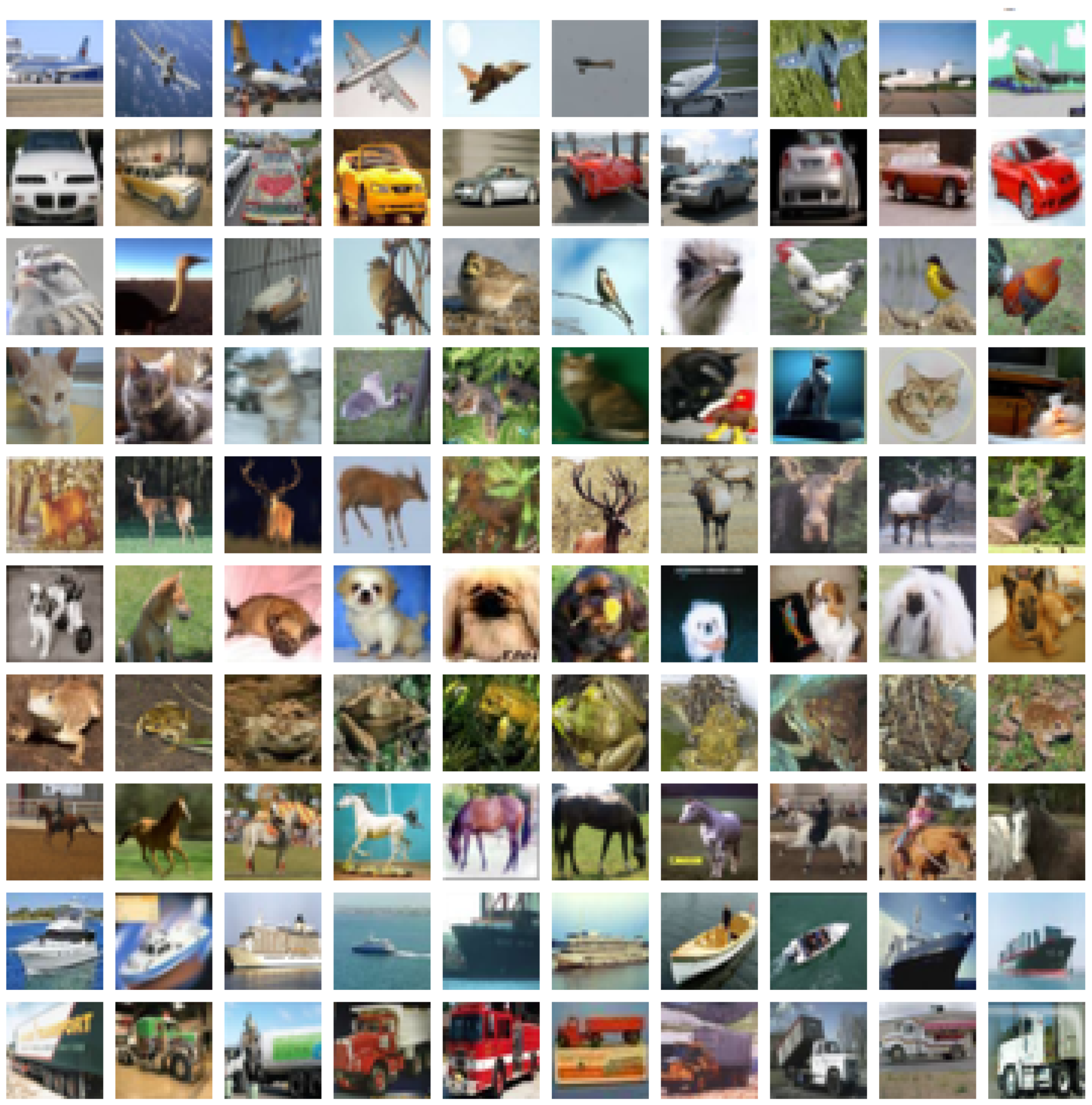
In this paper, we consider CNNs for image classification that is one of the most essential applications in image processing and computer vision [2,14]. Given an input image, the CNN classifies it into one of the predefined classes, e.g., an alphanumeric symbol for plate number detection [28,29] or a real-world object for object detection/recognition [9,10,11,12,13,14,15] as illustrated in Figure 1.
2.1. An Overview of the CNN Structure
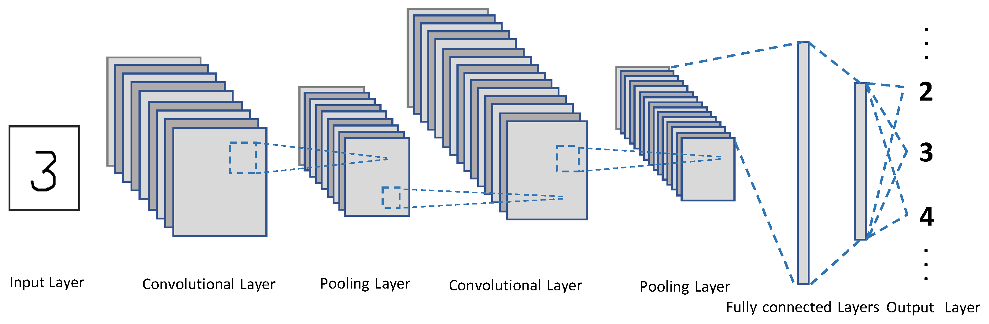
Figure 2 illustrates the general CNN architecture [2]. When an input image is provided, a CNN extracts features from the image using multiple pairs of convolutional and pooling layers and classify the image into a class using fully connected layers.
In general, a CNN model consists of an input layer, convolutional layers, pooling layers, fully connected layers, and an output layer. The input layer takes an input image and the output layer produces the predicted class, e.g., a pedestrian, bicycle, car, or truck. The number of convolutional and pooling layers vary depending on applications and accuracy requirements. Generally (but not necessarily), the deeper the higher is the accuracy with potentially diminishing returns.
In principle, deep learning is supervised learning. The architecture and complexity of a CNN model is determined by its hyper-parameters, such as the number of the layers and the sizes of the filter, stride, and pooling window (discussed shortly), which have different impacts on the execution time and inference accuracy. If the architecture of a CNN model is determined, the model is trained using a labeled data in the training set where each image in the data set is associated with the ground-truth label (class). The parameters, i.e., the weights of different features, should be determined in the training phase based on the back propagation and gradient descent algorithm applied to minimize the loss—the distance between the class predicted by the CNN and the true class [2,6].
A description of layers and key components in CNNs follows.
- Input layer [26,27,29]: In a CNN for computer vision, an image is represented by a 3D matrix defined by the image width, image height, and the depth of the channels, e.g., RGB. A gray scale image is stored as a 2D matrix. Images are pre-processed, if necessary, to conform to the width, height, and depth requirements and provided to the input layer. In CNNs, key operations, such as convolution and pooling to be discussed shortly, are independently applied to each channel. Therefore, for the sake of clarity, we mainly discuss convolution and pooling for 2D data in this section.
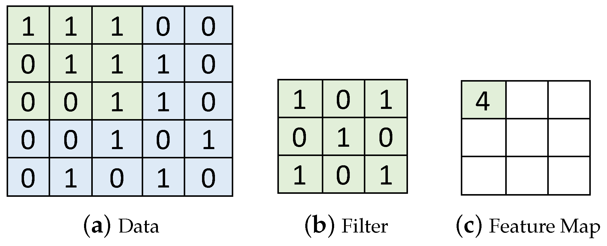
- Convolutional layers [2,31,32,33]: In a CNN, a convolution filter, also called a kernel, is applied to the input image. More specifically, element-wise multiplications between the filter and data in one segment are applied and the multiplication results are summed to produce one data in the feature map. For example, in Figure 3, a 3 × 3 kernel is applied to the first 3 × 3 segment in the input data. By performing the element-wise multiplications and sum, the first feature is produced in the feature map in Figure 3c. A new feature map is generated each time by sliding the filter a certain number of positions specified by the stride size (in Figure 3, stride = 1, that will produce nine convolutional results in the feature map). A convolutional layer usually uses multiple filters. As a result, it produces multiple feature maps and stacks them together [8]. A CNN usually consists of multiple convolutional layers. The first convolutional layers detect low level features, e.g., color, gradient orientation, and edges. The next layers detect middle-level features such as shapes. In addition, the following layers detect an object, e.g., a car. Kernel sizes and the number of convolutional layers are key hyper-parameters that determine the architectural configuration of convolutional layers. In addition, each convolutional output is provided to an activation function to expedite training. In this paper, we use ReRectified Linear Unit (LU) that is one of the most popular activation functions. It is an element-wise function applied to each data x produced by convolution; it simply returns . ReLU is popular since it is nonlinear and computationally efficient.
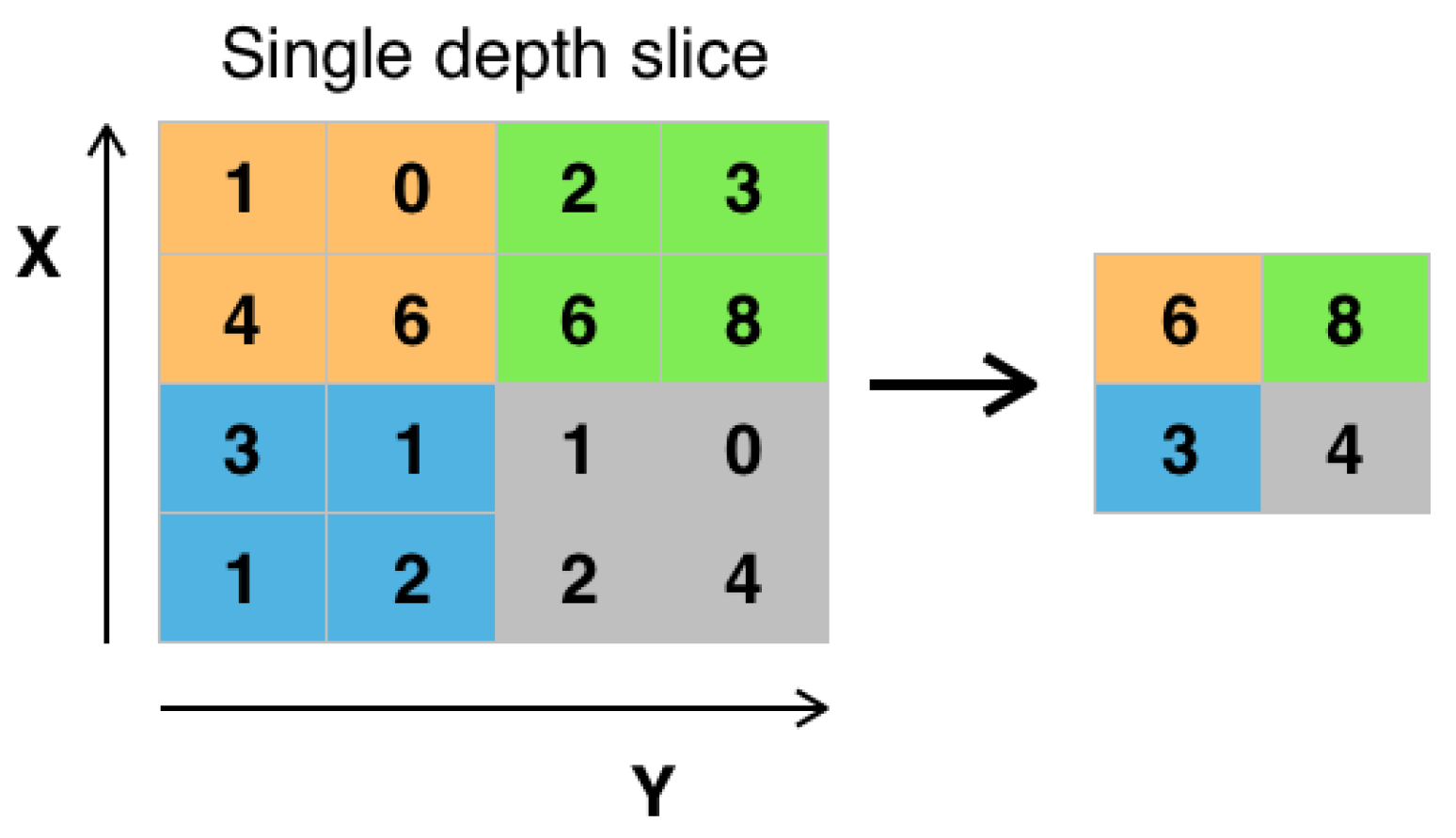
- Pooling layers [2,17]: The feature maps that is the output of one or more convolutional layer are fed into a pooling layer that, via downsampling, reduces the dimensionality and the risk of overfitting [1,34,35] where the CNN is memorizing the training data rather than generalizing the model to predict/infer the classes of new, unseen images. Max pooling and average pooling are the most common pooling techniques. For example, max pooing of size 2 × 2 with depth 1 and stride 2 is depicted in Figure 4. As shown in the figure, pooling keeps representative features, while halving the width and height. The pooling window size, stride, and number of pooling layers are important hyper-parameters that also affect the time and accuracy of image classification via CNNs.
- Fully connected layers [2]: In a CNN, feature maps processed through the convolution and pooling layers are flattened, i.e., converted to a single-dimension vector, and fed to the fully connected layers. Each neuron in the first fully connected layer then computes the weighted sum of the features provided to itself. The following fully connected layer computes the weighted sum of the output signals provided as the input to itself. This process is repeated through the fully connected layers.
- Output layer and training: By giving different features different weights, the convolutional and fully connected layers find the most correlated features to a particular class. In the prediction phase, the output layer gives the probabilities that the input image belongs to different predefined classes based on the detected features. For image classification with more than two classes, the softmax function [36] used in this paper is a common technique to compute the probabilities [6]. Finally, the class with the highest probability is selected and compared to the label, the ground truth. Based on the comparison results, the weights are adjusted to enhance the classification accuracy via back propagation [37] and gradient descent [38] techniques. By repeating the whole procedure for a big training data set, the CNN learns the model for a specific application, such as computer vision.
- CNN model evaluation: The accuracy of the trained CNN model is:where and represent the number of the images classified correctly and the total number of classified images, respectively.Specifically, accuracy is evaluated using the separate set of data, called the test set, the model has not seen during the training (for more details of CNNs, please refer to [2,6]). Following this approach, in Section 4, each data set is divided into the training set and test set. We use the training set to train our CNN models and use the test set to evaluate the generalizability of the models derived by our approach discussed in Section 3 in terms of the prediction accuracy and time.
2.2. Problem Formulation
In this paper, we assume that a soft real-time framework for image classification is deployed in an IoT gateway connected to one-hop (wired/wireless) cameras or in an edge server directly connected to the gateway. We consider a sporadic task model, since a camera can quickly determine whether there is any moving object using, for example, a motion sensor and submits an image to the server. Thus, the minimum inter-arrival time between two consecutive jobs of task for camera i is equal to the inverse of the frame rate of the camera. Upon the arrival of the image from camera i, the CNN is required to complete job to classify the image within the deadline = arrival time + , where is the relative deadline of . Our approach is orthogonal to real-time scheduling [40]. A popular scheduling algorithm, e.g., Earlier Deadline First (EDF), can be used to schedule image classification tasks.
We assume that the system is dedicated to (soft) real-time image classification, since image classification via deep learning within stringent timing constraints is computationally demanding. We also assume that input images from (wired/wireless) cameras may arrive late at the edge and image classification jobs can be preempted by higher priority jobs (if any) too. Given that, at run time, we dynamically select one of the CNN models expected to efficiently classify an input image with the best possible accuracy among the models in the system within the remaining time to the inference job deadline.
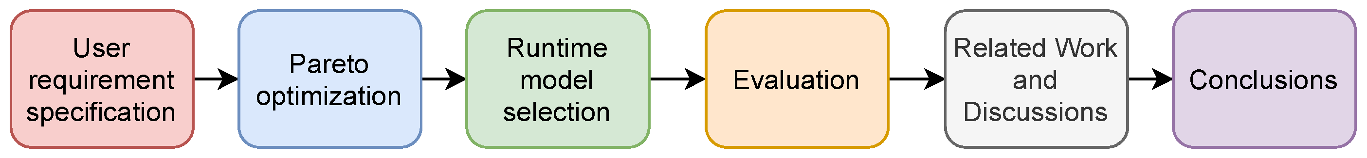
The block diagram in Figure 5 illustrates the proposed research step by step. First, our framework allows a user to specify the key requirements for adaptive real-time image classification, e.g., the required minimum accuracy, deadline, memory budget to store the adaptive CNN models, for an application of interest, e.g., traffic control or smart manufacturing. Second, we propose an effective approach that derives a set of -Pareto optimal CNN models to meet the user requirements. Third, we design a lightweight algorithm that dynamically chooses the CNN expected to support the highest accuracy subject to the remaining time to the deadline at runtime with minimal overheads. Fourth, the proposed approach and the two baselines described before are evaluated via extensive experiments. Furthermore, we discuss related work, advantages and limitations of the proposed approach, and future work issues followed by the conclusions.
3. Exploring CNN Models for Timely, Adaptive Image Classification
In this section, we discuss how to perform neural architectural search and find -Pareto optimal CNN models. Furthermore, we describe how to choose an appropriate -Pareto optimal model subject to the remaining time to the deadline at run time.
3.1. Overview
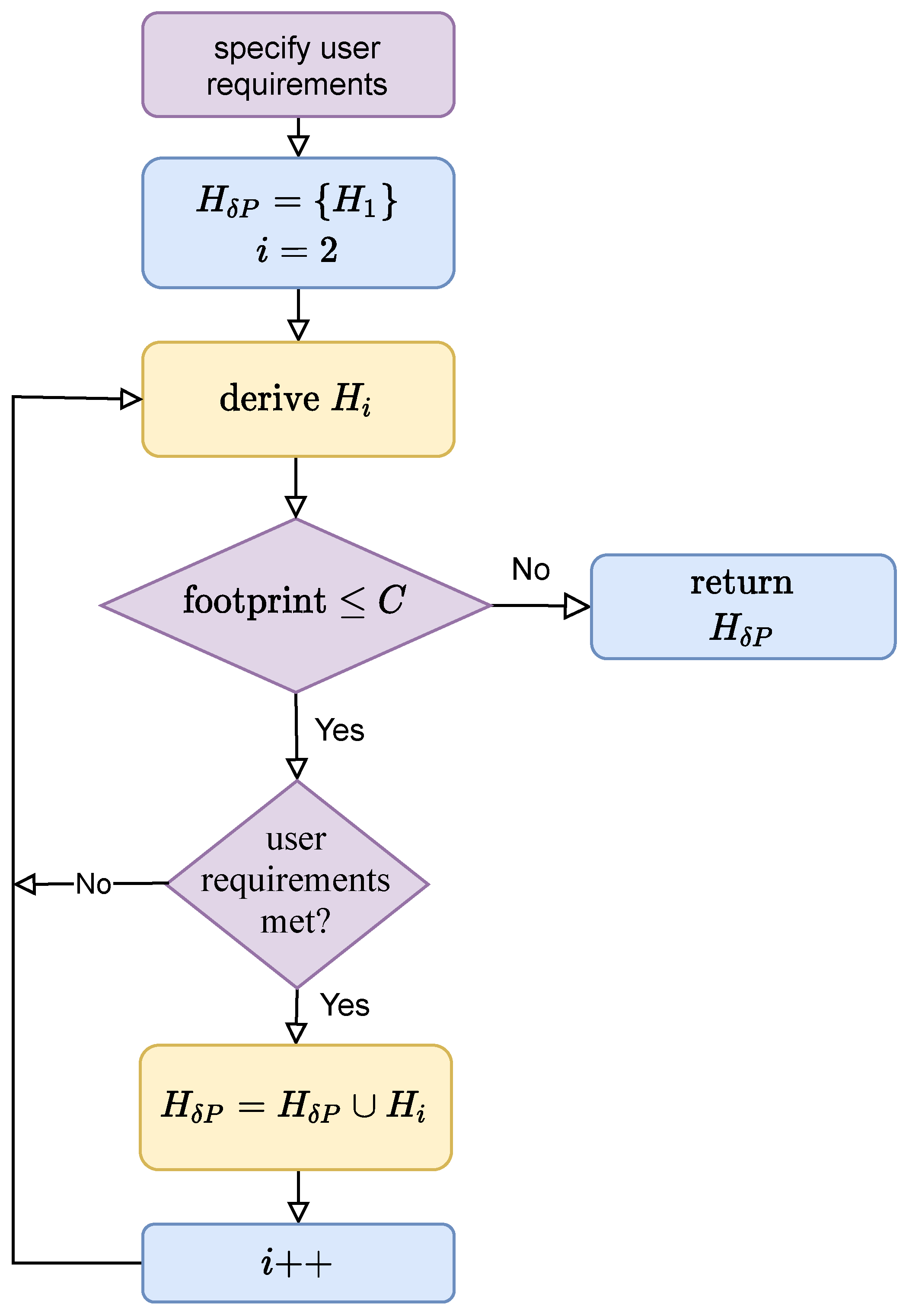
In our approach, a user (real-time application designer) aware of the semantics of a real-time data analytics application of interest specifies four user requirements: where is the minimum acceptable accuracy (for image classification in this paper), D is the inference deadline such as 1ms, C is the allowed amount of memory space to store CNNs with different inference times and accuracy, and is the minimum accuracy gain. To find Pareto optimal CNNs cost-efficiently, we take the following steps illustrated in Figure 6:
- We first derive a lightweight CNN, , whose accuracy is at least by exploring CNNs with different architectures (defined by their hyper-parameters).
- If the current set of Pareto efficient CNN models is where they are sorted in ascending order of the accuracy and inference time, we search for whose accuracy, , is higher than the accuracy of , , and its inference time, , is not longer than D by incrementally modifying the hyper-parameters of in the neighborhood of the search space to efficiently find .
- We repeat this process until we cannot find a new CNN such that and after a predetermined number of trials.
Figure 6.
Flowchart of Pareto Optimization. Our approach first finds the CNN, , whose accuracy (the user- specified minimum accuracy) and its execution time is not longer than the user-specified inference deadline D. It inserts into (the set of -Pareto optimal CNNs). It appends () to , if ’s inference time does not exceed D, where is the user-specified accuracy gain, and the total memory footprint of the -Pareto CNN models does not exceed the memory budget C. In the flowchart, the purple units specify and enforce user requirements for adaptive real-time image classification using our proposed approach, the blue boxes initialize and control the overall process, and the brown ones derive adaptive CNN models and add eligible CNNs that meet the user requirements into .

In this way, we build that meets the user requirements offline. Based on , we build the set of -Pareto optimal CNNs, . If , . We store in memory using no more than C bytes to support effective trade-offs between the inference time and accuracy at runtime, requiring no I/O to retrieve a CNN model. To classify an input image at time t, our approach efficiently selects the CNN model expected to provide the highest accuracy at t among the feasible CNN models in where the estimated inference time of an arbitrary CNN model is not longer than the remaining time to the deadline to meet stringent timing constraints. A more detailed description of deriving and selecting an appropriate CNN in at runtime for adaptive real-time image classification follows.
3.2. Finding -Pareto Optimal CNNs Offline
The CNN models in , the input to Algorithm 1, are sorted in ascending order of the accuracy and inference time. In line 1 of Algorithm 1, we initialize the set of -Pareto optimal CNNs: = . In lines 2–4, we initialize several variables: the number of CNNs in , the total memory footprint, and the highest accuracy provided by the CNNs currently in .
In lines 5–10, is appended to , if its accuracy is higher than the accuracy of the CNN most recently appended to by at least and the user-specified memory budget, C, will not be exceed after adding to . Finally, in line 11, the algorithm returns and (the number of the CNNs in ) where .
We only store in the edge server for efficient time vs. accuracy trade-offs at run-time. A user (i.e., an application designer) can specify and C in Algorithm 1 to control based on application requirements and the available memory space to store CNNs. Furthermore, the prediction time of every CNN in and does not exceed the user-specified deadline D by construction as discussed in the previous subsection.
| Algorithm 1: Deriving -Pareto Optimal CNNs Offline. |
 |
Given N input CNNs that are Pareto optimal, the time complexity of Algorithm 1 is . The time complexity for sorting is and the time complexity for building is that is dominated by .
3.3. Efficient Run-Time Selection of a CNN for Timely Image Classification
When an input image should be classified by a sporadic task instance , the real-time image classification system picks , one of the -Pareto CNN models stored in the system, using Algorithm 2. The algorithm simply looks up the table of the -Pareto optimal CNNs in and picks the CNN, , expected to support the highest possible accuracy subject to , i.e., the remaining time to the (absolute) deadline of the inference job :
where is the lookup table for the CNNs in . Subsequently, the system classifies the image using . (If the inference time of every CNN in is longer than the remaining time to the deadline, Algorithm 2 returns that has the shortest execution time in ).
| Algorithm 2: Run-Time Selection of a CNN Model. |
 |
In this paper, we require be a small constant. We make this design choice, since the algorithm needs to run frequently to support high accuracy image classification subject to timing constraints. Thus, the time complexity of Algorithm 2 is .
4. Evaluation Results
In this section, we first evaluate the impacts of hyper-parameters on the accuracy and latency for predictions using two popular data sets to verify our assertion that hyper-parameters affect the inference time and accuracy and analyze which hyper-parameters have more impacts. After that, we evaluate the feasibility and effectiveness of our approach in comparison to layer-wise adaptation, e.g., [24,25]. Since the source code of [24,25] was not available, we have used the depth of a CNN as another hyper-parameter in our model search and evaluation. In this paper, we have used TensorFlow [22] to implement our CNN models.
4.1. Data Sets and Hyper-Parameters
4.1.1. MNIST Data Set
The MNIST data set of handwritten digits [26] consists of 60,000 samples in training set and 10,000 samples in the test set. As summarized in Table 1, all the CNN models we trained for MNIST data set consist of two convolutional and ReLU layers, two pooling layers, and two fully connected layers where the number of neurons in the second fully connected layer is a half of that in the first fully connected layer. We have fixed the basic CNN architecture using these hyper-parameters, since we have achieved relatively high accuracy that ranges between 0.9 and 0.99 with different execution times for different values of the other hyper-parameters—different kernel sizes, pool sizes, stride sizes, and numbers of neurons in the fully connected layers.
For training, we have performed 40,000 iterations. The batch size is 64; therefore, the model is updated after processing 64 random samples via the gradient descent algorithm [6]. The number of channels in the first and second convolutional layer are 16 and 36, respectively. The learning rate controls how quickly a model adjusts the weights. It is typically a small positive number less than 1. For the MNIST data set, we use the learning rate of . For training and inferences using the MNIST data set, we have used a machine with 4 cores and 8GB memory to mimic an IoT gateway or a low-end edge server such as [41].
4.1.2. CIFAR-10 Data Set
The CIFAR-10 data set [27] consists of 50,000 images in the training set and 10,000 images in the test set. Every image is color and labeled: it belongs to one of the 10 different classes of objects. As CIFAR-10 data are more complex and harder to train and perform predictions, we consider a more diverse set of hyper-parameters to support systematic trade-offs between the inference time and accuracy. Table 2 shows the hyper-parameters of the bare-bone CNN architecture. Based on these hyper-parameters, we train many models that use different kernel, pool, and stride sizes to empirically evaluate their impacts on inference time and accuracy. Furthermore, we consider different numbers of convolutional, ReLU, and pooling layers.
To train a model, we use 150 epochs where each epoch processes all the images in the training set instead of using small batches different from what we have done for the MNIST data set. The initial learning rate is but it is reduced to after 100 epochs to make the weight adjustments less aggressive in the later part of training. As training and inference is more challenging for the CIFAR-10 data set, we use a more powerful machine with the 16 core Intel Xeon E5-2667 processor and 32GB memory to mimic a real-time edge server for classifying images from embedded cameras.
For each measurement of the inference time, we have used 1000 randomly selected images in the test set of the MNIST or CIFAR-10. We report the results of 20 such measurements using box plots, since the execution time varies even for the same CNN model with the same hyper-parameters and parameters (weights). To measure the inference accuracy, however, we have used the entire data in the test set following a common practice in machine learning literature [2]; therefore, there is only one accuracy measurement with respect to a specific set of hyper-parameters (and parameters). For brevity, Table 3 introduces a few notations that represent the hyper-parameters varied for experiments. In the following subsection, we evaluate the impacts of , and d on the prediction accuracy and time.
4.2. Impacts of Hyper-Parameters on the Inference Time and Accuracy
4.2.1. Impacts of the Convolutional Kernel and Stride Sizes
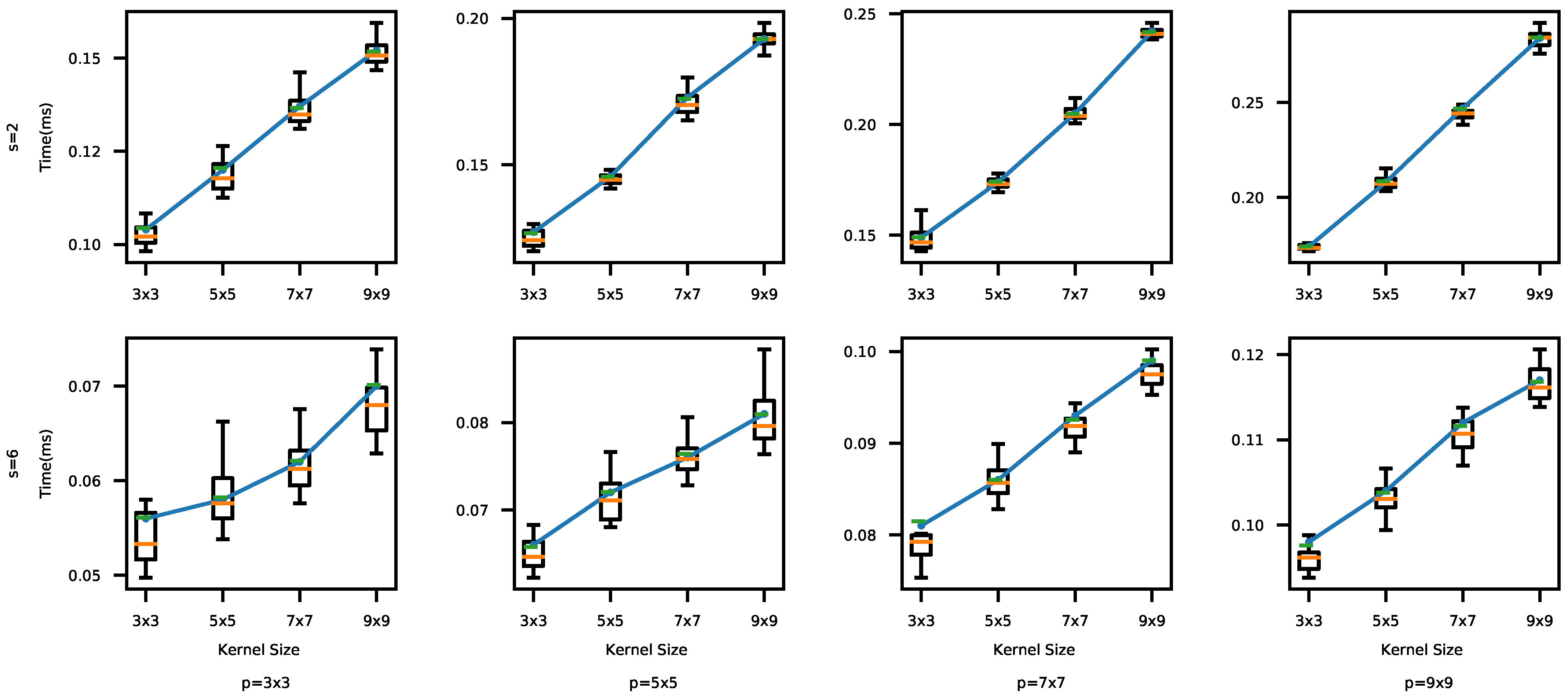
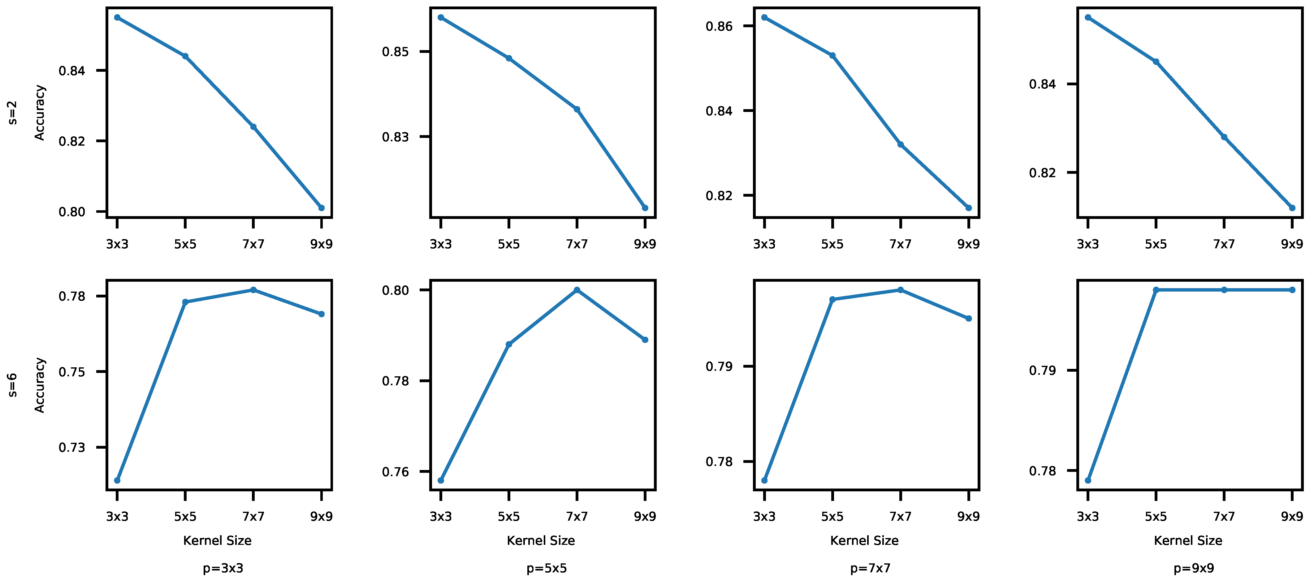
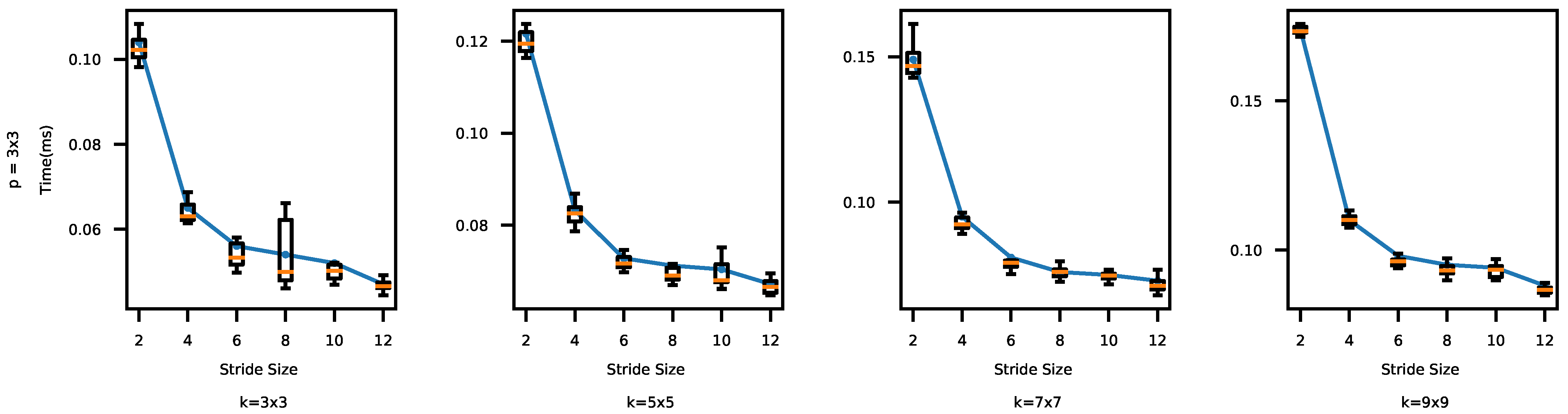
First, we evaluate the impact of the convolutional kernel size k on the prediction time and accuracy. We measure the time and accuracy using four different kernel sizes in the convolutional layers, , and 9 × 9, for each combination of p, s, and f (defined in Table 3). More specifically, we have used 72 different combinations of and f for each k. For the clarity of the presentation, we only plot the most representative results in Figure 7 and Figure 8 where .
From Figure 7 and Figure 8, we observe that the accuracy and execution time for is generally higher than those for , since a small stride performs relatively fine-grained data analysis via more convolutions. As shown in Figure 7, the execution time generally increases as the kernel size increases too due to the higher computational loads. In Figure 8, however, the accuracy does not show an obvious trend for different kernel sizes. For , the accuracy actually decreases as k increases, because there could be too much overlapped data between adjacent kernel executions as k increases. For , the accuracy initially increases but eventually plateaus or even drops as depicted in Figure 8. When k is relatively small (e.g., k = 3 × 3), the big stride skips certain data, resulting in low accuracy. As k increases, each kernel execution processes a bigger data block so that important features are skipped less; therefore, the accuracy increases. However, it becomes to process overlapped data repeatedly when , increasing the likelihood of a drop in accuracy. Our experiments using the MNIST data set have shown similar results.
For the CIFAR-10 data set, the accuracy differences between the tested CNNs with different kernel and stride sizes range between 1.50 and 9.25%. The biggest execution time gap between the CNN models with different kernel sizes is . For the MNIST data set, the impacts on the accuracy and execution time are between 0.1 and 3.65% and at most , respectively. The difference of the results between the different kernel and stride sizes is less noticeable for MNIST, because the data set is less complex and, therefore, it is easier to achieve high accuracy using a relatively simple CNN architecture.
4.2.2. Impacts of the Pooling Window and Stride Sizes
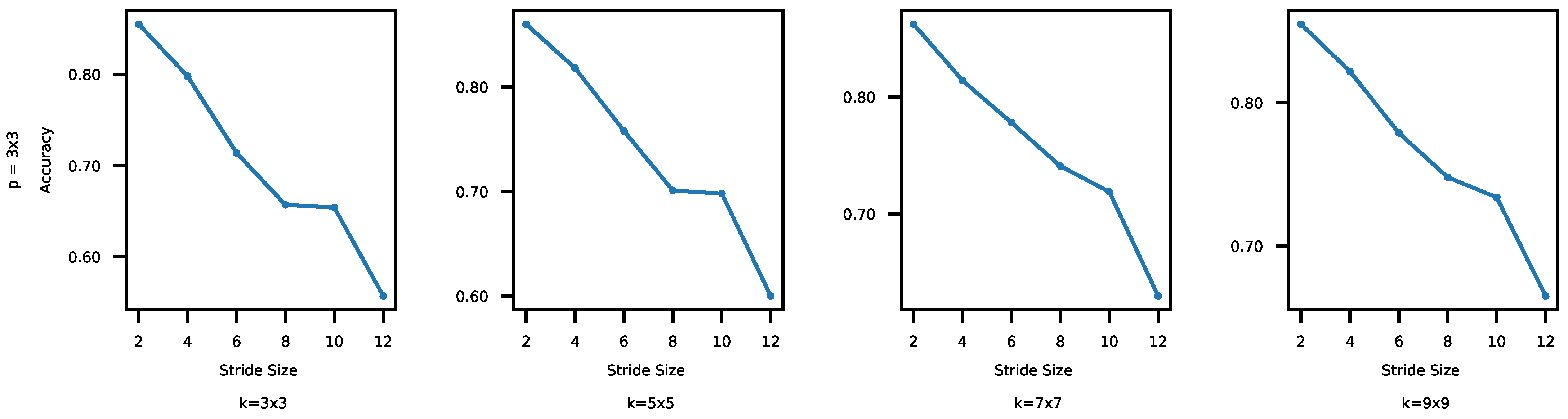
In CNNs, pooling is used for downsampling to reduce redundant features, keeping representative ones. In this set of experiments, we vary the pooling window and stride sizes in the pooling layers that affect downsampling together. We evaluate their impacts on the inference time and accuracy. Specifically, we consider 3 × 3, 5 × 5, 7 × 7, and 9 × 9, and s = 2, 4, 6, 8, 10, and 12. For each p (pooling window size), we have used 72 combinations of k, s, and f. In addition, to evaluate possible impacts on time and accuracy of each s (stride size), we have considered 48 combinations of and f. Especially, we present the results for ; the results for the other pooling window sizes were similar.
In Figure 9 and Figure 10, both the time and accuracy drop as s increases. In Figure 9, the time initially decreases as s increases and then the trend slows down. This is because less computation is needed as s increases initially. When in Figure 9, however, data skipping cannot make the models run much faster, because the basic computations in the convolutional and pooling layers do not decrease significantly. On the other hand, skipping results in loss of features, incurring accuracy drops. As a result, in Figure 10, the accuracy drops almost linearly as the stride size increases.
Interestingly, the inference time varies more widely for the different pooling window and stride combinations than it did for the different combinations of the kernel and stride sizes (discussed in Section 4.2.1). For the CIFAR-10 data set, the accuracy changes between 1.4 and 11.02% across all the CNNs tested in this section (1.25–9.25% in Section 4.2.1). The biggest difference in the inference time between any two different CNNs is 38.77% ( in Section 4.2.1). We think this is because the goal of pooling is downsampling [6]. Thus, combinations of pooling window and stride sizes give the real-time image classification system more adaptability and control in terms of time vs. accuracy trade-offs. We observe similar patterns for MNIST: the impact on the accuracy and latency are between 0.1 and 3.99% (0.1–3.65% in Section 4.2.1) and at most 21.9% (19.86% in Section 4.2.1), respectively.
4.2.3. Impacts of the Fully Connected Layers
In this subsection, we evaluate the accuracy and time for different sizes of the first fully connected layers that range between114 and 144 and 320–448 neurons for MNIST and CIFAR-10, respectively (the second fully connected layer uses a half of the neurons as discussed in Section 4.1.1). However, we have not observed any clear pattern: using more neurons in the fully connected layers does not necessarily increase the accuracy or time to a noticeable degree. We think this is because main computations occur in the convolutional and pooling layers in a CNN. Furthermore, certain connections between the neurons in the fully connected layers may have little impact on accuracy due to the small weights. The number of neurons in the fully connected layers may have more impact on the time and accuracy in different deep learning models than CNNs. However, it is beyond the scope of the paper as we focus on adaptive real-time image classification using CNNs in this paper.
4.2.4. Impacts of the Total Depth
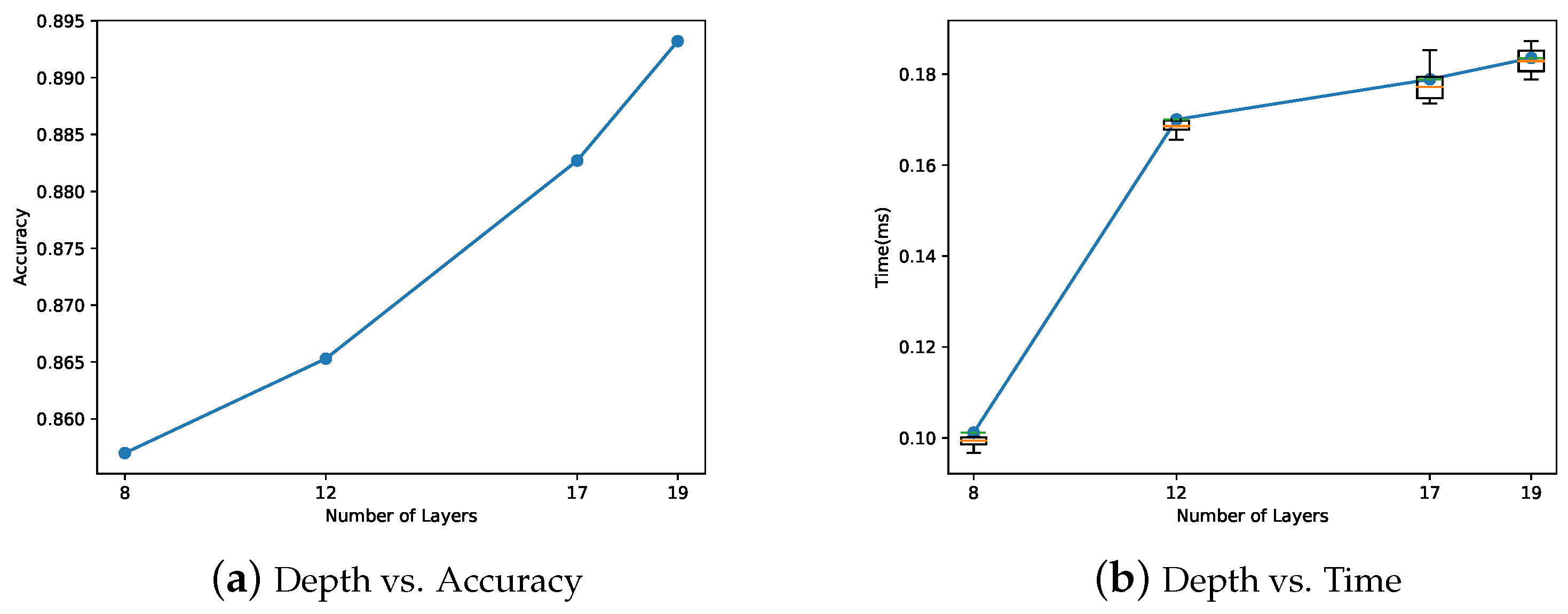
In this set of experiments, we evaluate impacts of the total depth of a CNN on the inference time and accuracy. We use several different depths, i.e., the total number of layers in the tested CNNs, summarized in Table 4 for the CIFAR-10 data set (we have achieved up to 0.99 accuracy using a CNN of depth 8 outlined in Table 1 for the MNIST data set. Thus, we do not consider increasing its depth any further). We set k = 3 × 3, p = 2 × 2, s = 2, and f = 512 to compare the CNNs with different depths on the common basis. We have trained each model and tuned their parameters independently.
In Figure 11, as the depth increases from 8 to 19, the accuracy and median time for an inference increases by approximately 0.036 and 0.08 ms, respectively. Although the accuracy is increased by 3.6%, the median execution time for one inference increases by more than 80%. From this, we observe that increasing the total depth of a CNN is a relatively expensive and less cost-effective option. Essentially, real-time image classification by only adapting the number of the layers (e.g., [24,25]) to execute at runtime is substantially more restricted and provides a much narrower scope of adaptation than our approach does. Thus, our approach is more cost-effective.
4.2.5. Summary of Time vs. Accuracy Relationships
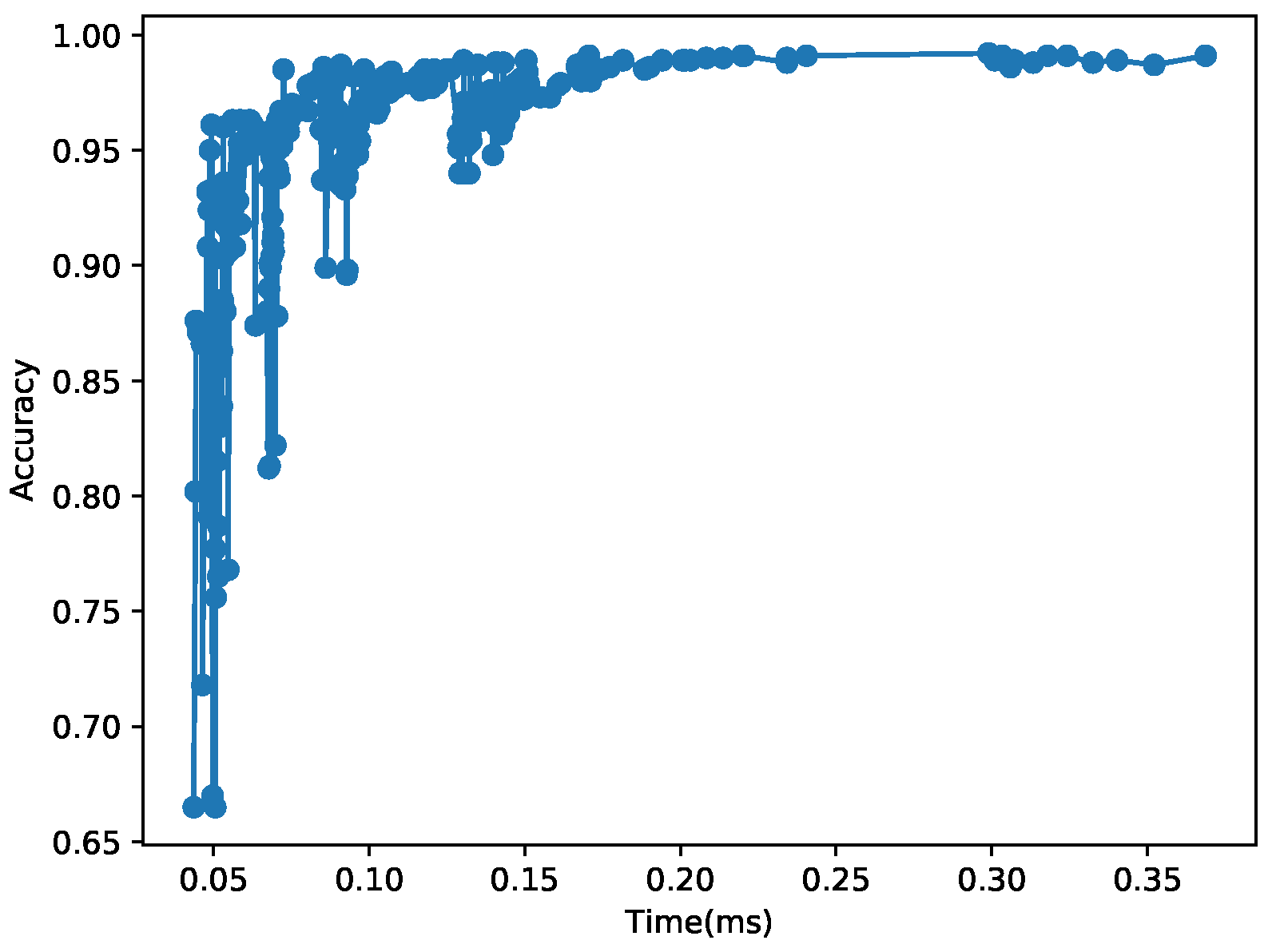
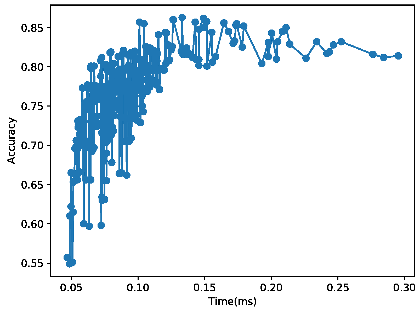
Figure 12 and Figure 13 plot the relationships between the inference time and accuracy for all the combinations of different hyper-parameters tested in this section. Each data point in the 2D figures shows the time and accuracy of each CNN fully configured by its hyper-parameters (and weights). In the figures, the relationship between the CNN execution time and accuracy is nonlinear and considerably irregular in that there are many zigzags and wide swings of accuracy for similar execution times. Hence, it is naive and often erroneous to assume that a longer execution time definitely leads to higher accuracy. To address the issue, in this paper, we explore organized trade-offs between time and accuracy for real-time image classification to support monotonically increasing accuracy with respect to the execution time.
4.3. Effectiveness of Our Model Selections and Adaptation
Given the hundreds of CNN models whose inference times and accuracy are plotted in Figure 12 and Figure 13, our approach picks only a few -Pareto optimal CNN models for cost-efficient real-time image classification as discussed next.
4.3.1. Evaluation Using MNIST
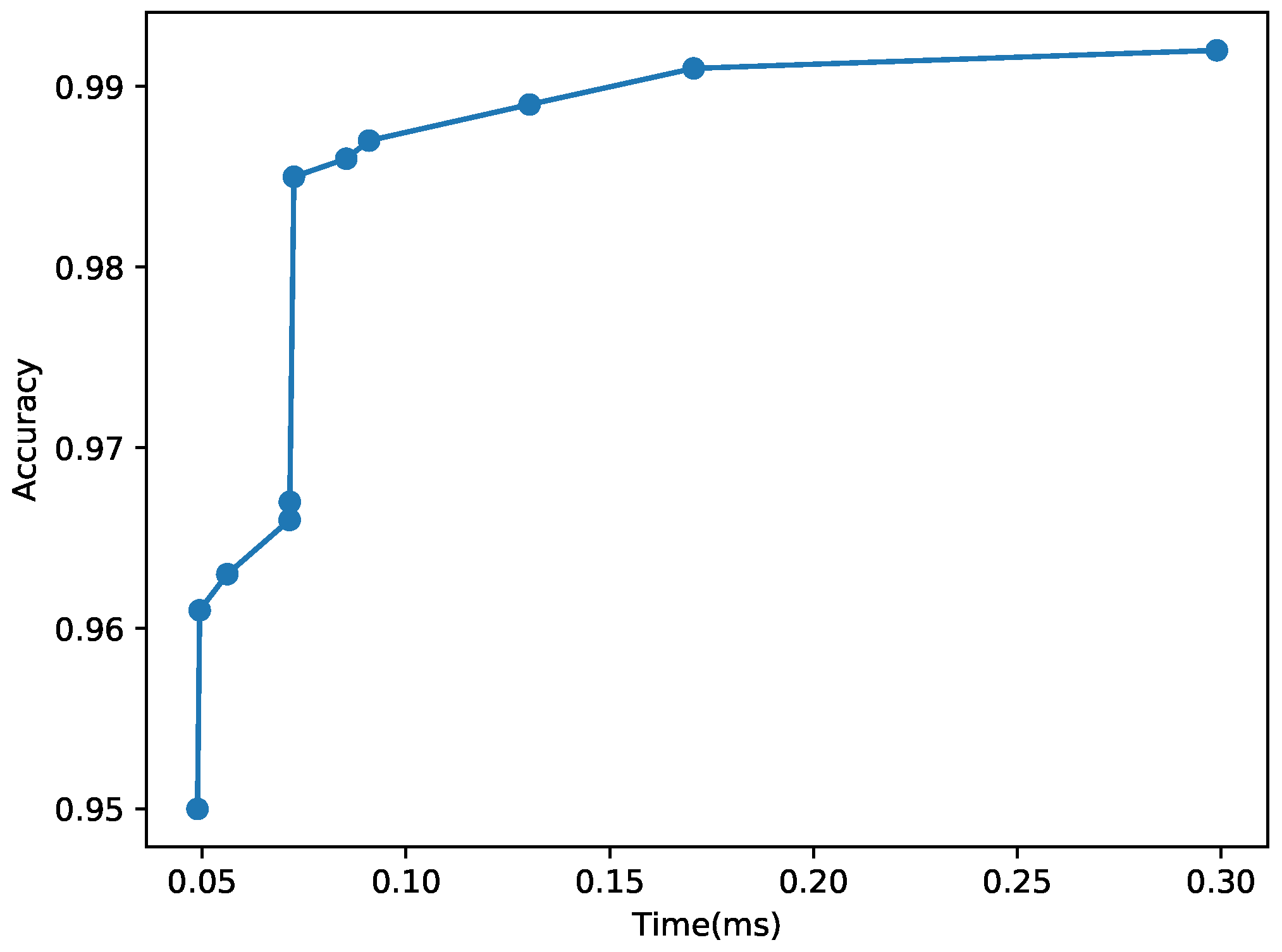
To evaluate the effectiveness of our approach, let us consider an example user requirement specification for MNIST: , , ms, and MB. To meet the specified user requirements, we first derive that supports , D, and C. By incrementally modifying the hyper-parameters of in the neighborhood of , we derive the set of 11 Pareto optimal CNN models, , in ascending order of accuracy and inference times as illustrated in Figure 14 and summarized in Table 5, while discarding Pareto-inefficient CNNs that fail to support monotonically increasing accuracy for longer inference times. Furthermore, using Algorithm 1, we extract the set of -Pareto optimal CNNs, , boldfaced in Table 5. Our first baseline, which is a common approach for image classification via deep learning, only uses that supports the highest accuracy without any runtime adaptation via imprecise computation considering the remaining time to the deadline. The accuracy of and in is lower than that of by 0.042 and 0.007, but their inference times are only 16.8% and 25% of the baseline, respectively. Therefore, our real-time image classification system can pick among using Equation (2) based on the remaining time to the deadline, if necessary, to meet stringent timing constraints of real-time image classification tasks for a relatively small accuracy loss when or is chosen. In Table 5, every inference time (1 ms). Moreover, the total memory consumption to store is 6.625 MB . Therefore, our approach meets the user required , , D, and C by constructing .
4.3.2. Evaluation Using CIFAR-10
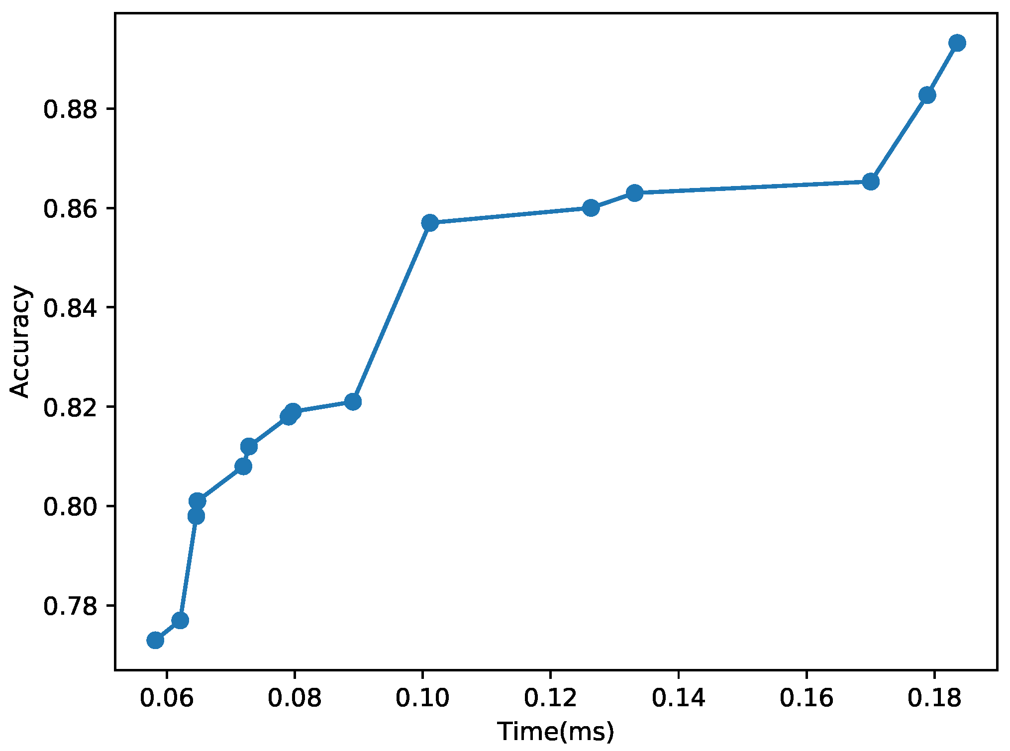
For the evaluation using CIFAR-10, let us consider an example user-specification: , , ms, and MB. By incrementally modifying the hyper-parameters of , we derive the set of 11 Pareto optimal CNN models, , with the increasing accuracy and inference time as shown in Figure 15 and summarized in Table 6, while discarding the Pareto-inefficient CNNs that fail to support increasing accuracy for longer inference times. In addition, using Algorithm 1, we extract the set of -Pareto optimal CNNs, , boldfaced in Table 6. Comparing to the baseline that only uses , the accuracy of and is lower by 0.085 and 0.036, but their inference times are only 39.2% and 55.1% of the baseline, respectively. Thus, our real-time image classification system can efficiently pick among using Equation (2), if necessary, to meet tight timing constraints. In Table 5, every inference time (1 ms). Furthermore, the total memory consumption to store is 48.857 MB . Hence, our approach meets the user-specified , D, C, and requirements by building .
4.3.3. Summary of the Effectiveness and Overhead of Our Approach
Unlike another baseline that considers the depth of the CNN for adaptation [24,25], we can consider and leverage several CNNs with the same number of layers too, such as the CNNs in Table 5 and Table 6, if they meet the user requirements. Thus, our approach is more flexible and cost-effective as discussed before. Comparing to the first baseline that only uses , our approach consumes additional 3.067 MB and 9.899 MB to keep and for MNIST and CIFAR-10 in memory, respectively, (Table 5 and Table 6). By comparing Figure 12 and Figure 13 to Table 5 and Table 6, we observe that Algorithm 1 reduces the total number of candidate models for runtime adaptation by two orders of magnitude. Furthermore, Algorithm 2 for dynamic adaptation is O(1) as discussed in Section 3. It selects a CNN in expected to meet D only in 7–8 ns and 17–20 ns for MNIST and CIFAR-10, respectively. The additional memory consumption and latency of our adaptive approach is acceptable in modern edge gateways or servers. Overall, our approach has significant advantages over the common baseline approaches for the relatively small overhead.
5. Related Work
In early studies, accuracy is the standard metric to evaluate performance in machine learning applications [9,13]. Most object detection papers [9,10,11,12,13,14,15] focus on how to detect objects with high accuracy. In recent works, e.g., R-FCN [11], SSD [42], and YOLO [9], however, not only accuracy but also the frame rate is evaluated. In [13], trade-offs between the accuracy and frame rate are evaluated for three different neural networks, R-FCN [11], R-CNN [12], and SSD [42]. In this paper, we derive a set of -Pareto CNNs that satisfy the user-specified accuracy and memory requirements to efficiently meet stringent timing constraints of real-time image classification based on imprecise computation, since the average frame rate over an extended time interval may fail to measure and control transient fluctuations of latency (and timeliness) of individual inferences. Thus, our approach is complementary to these approaches.
Recently, real-time image classification and object detection are drawing increasing attention [24,25,43,44]. The key difference between our proposed approach and such works is that we systematically study impacts of hyper-parameters on the accuracy and execution time of CNNs to support a monotonic increase in accuracy for a longer execution time with little overhead at runtime. There are existing works on evaluation of CNN hyper-parameters [13,45]; however, they do not consider timing constraints. In [13], different types of activation functions and classifiers are evaluated; however, we do not consider them since they do not affect execution times significantly.
Partial execution of some neurons or layers in CNNs based on the input or deadline has been considered. Input-dependent execution has been widely used in computer vision, such as cascaded detectors [46,47]. In dynamic Deep Neural Networks () [48], in addition to normal neurons, there are control nodes that dynamically decides to skip neurons so that the execution time can be adjusted accordingly at run-time based on input. However, does not deal with time vs. accuracy trade-offs to meet stringent timing constraints for real-time image classification.
Deadline-based dynamic frameworks make the neural network model dynamically/ selectively execute a subset of layers. AnytimeNet [24] is a framework that enables gradual insertion of additional layers in an attempt to enhance accuracy if time permits. In multi-path neural networks [25], a model is trained with multiple paths which contain different numbers of layers. At run-time, it is possible to change paths based on deadlines. In [49], a ResNet [50], is divided into a mandatory part and an optional part where the former is always executed, but the latter is run when enough time is available. In fact, Refs. [24,25,49] are most closely related to our work. Our work is, however, significantly more comprehensive than them in that the number of layers in a or the number of resblocks in a ResNet (CNN) is only one hyper-parameter whose applicability is relatively limited as thoroughly analyzed in Section 4. Depending on applications, a shallow neural network may provide high accuracy. In this paper, for example, a CNN with only eight layers in total supports over 0.99 accuracy for the MNIST data set. In [51], a CNN with only two hidden layers supports wireless channel state information classification with up to 0.98 accuracy. Adding more layers in such applications will increase the inference time with largely diminishing returns. Thus, we consider not only the number of layers but also the other important hyper-parameters, such as the kernel size, pooling window size, stride, and number of neurons in the fully connected layers, to support more robust, cost-efficient trade-offs between the inference time and accuracy. Thus, our work is complementary to them.
6. Discussion
Generally speaking, research on real-time machine learning explored in this paper is in an early stage with many open issues [52]. Supporting real-time machine learning is a challenging problem, since machine learning methodologies, e.g., deep learning, are computationally expensive. Further, new deep learning models are becoming increasingly more complicated to enhance the prediction performance. In this regard, the advantage of the proposed approach is providing systematic, robust trade-offs between the accuracy and timeliness of real-time image classification based on deep learning. Our design goal was to minimize the complexity and resulting uncertainties detrimental in safety-critical real-time systems, e.g., traffic control and smart manufacturing.
A drawback of our approach is the increased memory consumption to store multiple CNN models, even though the memory overhead is acceptable as analyzed in Section 4. To further reduce the memory consumption, several techniques, such as model pruning [53] and compression [54], can be applied to prune less important weights and compress them. Another limitation of the proposed approach is that the trained models are fixed. As a result, the prediction performance may drop, if the real-world environment, e.g., traffic status or lighting conditions, change dramatically. To address this issue, incremental learning [55] can be applied to continually update the model as necessary. A related challenge is how to support incremental learning without impairing the timeliness and current prediction accuracy. A thorough investigation is reserved for future work.
In addition, our approach could be integrated with other advanced works, such as [56,57,58], to create synergy. For example, our approach can be combined with [56] to diagnose faulty machine components in real-time in a smart factory. Furthermore, it can be synthesized with [57,58] to support efficient real-time video compression and nighttime image classification, respectively. These issues are reserved for future work.
7. Conclusions and Future Work
Although deep learning can significantly improve real-time applications, e.g., traffic control or smart manufacturing, it is computationally demanding. As a result, deadlines could be missed, raising potential safety issues. To shed light on the problem, we design a new adaptive approach for soft real-time image classification based on imprecise computation. In this paper, we analyze the relationship between the prediction time and accuracy of many CNN models offline. We then construct a set of -Pareto optimal CNNs that support higher accuracy for a longer execution time. At run-time, our approach efficiently selects the CNN model expected to support the highest accuracy for image classification subject to the inference deadline among the stored -Pareto optimal CNNs. In our evaluation undertaken using two popular data sets, we verify that our approach can find a set of -Pareto CNN models for cost-efficient time vs. accuracy trade-offs. For the MNIST data set, the accuracy and inference time of the models range between 48.84 and 298.99 s and 0.95–0.992. For the CIFAR-10 data set, the accuracy and inference time range between 71.97 and 183.55 s and 0.808–0.893. In contrast, the vanilla baseline that uses one non-adaptive model cannot support dynamic runtime adaptation to meet timing constraints. Designing the second baseline that only adapts the number of layers in a single CNN model, if necessary, to meet timing constraints is considerably less effective and flexible than our approach. By increasing the number of layers from 8 to 19, its inference time is increased by more than , while the accuracy is improved by 3.6% only. In our approach, however, we enhance the accuracy by 4.9% and 8.5%, while increasing the inference time by and using 8 and 19 layers, respectively. Thus, using the same number of layers, we can support higher accuracy than the layer-wise adaptation method, while further enhancing the accuracy when sufficient time is remaining till the deadline. Furthermore, our approach is lightweight with little overhead. In general, real-time sensor data analytics via machine learning is an emerging topic. In this paper, we have performed an early work on systematic trade-offs between the time and accuracy for image classification. In the future, we will continue to investigate related research issues including the ones discussed in Section 6.
Author Contributions
F.C. has designed the framework and CNNs. He has also done performance evaluation. K.-D.K. has advised them to formulate the research problem investigated in this paper. He has also helped them to design and analyze the proposed approach and to write the paper. All authors have read and agreed to the published version of the manuscript.
Funding
This research was funded by National Science Foundation: CNS-2007854.
Institutional Review Board Statement
Not applicable.
Informed Consent Statement
Not applicable.
Data Availability Statement
Acknowledgments
This work was supported, in part, by the National Science Foundation under Grant No. CNS-2007854.
Conflicts of Interest
The authors declare no conflict of interest. The funding sponsor had no role in the design of the study; in the collection, analyses, or interpretation of data; in the writing of the manuscript, and in the decision to publish the results.
References
- Bishop, C.M. Pattern Recognition and Machine Learning; Springer: Berlin/Heisenberg, Germany, 2006. [Google Scholar]
- Zhang, Z.; Cui, P.; Zhu, W. Deep Learning on Graphs: A Survey. IEEE Trans. Knowl. Data Eng. 2020. [Google Scholar] [CrossRef] [Green Version]
- Belinkov, Y.; Glass, J. Analysis Methods in Neural Language Processing: A Survey. Trans. Assoc. Comput. Linguist. 2019, 7, 49–72. [Google Scholar] [CrossRef]
- Bhandare, A.; Bhide, M.; Gokhale, P.; Chandavarkar, R. Applications of Convolutional Neural Networks. Int. J. Comput. Sci. Inf. Technol. 2016, 7, 2206–2215. [Google Scholar]
- Zhang, Q.; Yang, L.T.; Chen, Z.; Li, P. A survey on deep learning for big data. Inf. Fusion 2018, 42, 146–157. [Google Scholar] [CrossRef]
- Goodfellow, I.; Bengio, Y.; Courville, A. Deep Learning; MIT Press: Cambridge, MA, USA, 2016. [Google Scholar]
- Wu, Z.; Pan, S.; Chen, F.; Long, G.; Zhang, C.; Yu, P.S. A Comprehensive Survey on Graph Neural Networks. IEEE Trans. Neural Networks Learn. Syst. 2021, 32, 4–24. [Google Scholar] [CrossRef] [Green Version]
- Xue, B.; Zhang, M.; Browne, W.N.; Yao, X. A Survey on Evolutionary Computation Approaches to Feature Selection. IEEE Trans. Evol. Comput. 2016, 20, 606–626. [Google Scholar] [CrossRef] [Green Version]
- Huang, R.; Pedoeem, J.; Chen, C. YOLO-LITE: A Real-Time Object Detection Algorithm Optimized for Non-GPU Computers. In Proceedings of the 2018 IEEE International Conference on Big Data (Big Data), Seattle, WA, USA, 10–13 December 2018; pp. 2503–2510. [Google Scholar]
- Jiao, L.; Zhang, F.; Liu, F.; Yang, S.; Li, L.; Feng, Z.; Qu, R. A Survey of Deep Learning-Based Object Detection. IEEE Access 2019, 7, 128837–128868. [Google Scholar] [CrossRef]
- Han, J.; Zhang, D.; Cheng, G.; Liu, N.; Xu, D. Advanced Deep-Learning Techniques for Salient and Category-Specific Object Detection: A Survey. IEEE Signal Process. Mag. 2018, 35, 84–100. [Google Scholar] [CrossRef]
- Ren, S.; He, K.; Girshick, R.; Sun, J. Faster R-CNN: Towards Real-Time Object Detection with Region Proposal Networks. IEEE Trans. Pattern Anal. Mach. Intell. 2017, 39, 1137–1149. [Google Scholar] [CrossRef] [Green Version]
- Huang, J.; Rathod, V.; Sun, C.; Zhu, M.; Korattikara, A.; Fathi, A.; Fischer, I.; Wojna, Z.; Song, Y.; Guadarrama, S.; et al. Speed/accuracy trade-offs for modern convolutional object detectors. In Proceedings of the IEEE Conference on Computer Vision and Pattern Recognition, Honolulu, HI, USA, 21–26 July 2017. [Google Scholar]
- Russakovsky, O.; Deng, J.; Su, H.; Krause, J.; Satheesh, S.; Ma, S.; Huang, Z.; Karpathy, A.; Khosla, A.; Bernstein, M.; et al. ImageNet Large Scale Visual Recognition Challenge. Int. J. Comput. Vis. 2015, 115, 211–252. [Google Scholar] [CrossRef] [Green Version]
- Dai, J.; He, K.; Sun, J. Instance-Aware Semantic Segmentation via Multi-task Network Cascades. In Proceedings of the the IEEE Conference on Computer Vision and Pattern Recognition, Las Vegas, NV, USA, 27–30 June 2016. [Google Scholar]
- Landing AI. Available online: https://landing.ai/ (accessed on 20 February 2021).
- Zeiler, M.D.; Fergus, R. Visualizing and understanding convolutional networks. In Lecture Notes in Computer Science (Including Subseries Lecture Notes in Artificial Intelligence and Lecture Notes in Bioinformatics); 8689 LNCS; Springer: Berlin/Heisenberg, Germany, 2014; pp. 818–833. [Google Scholar]
- Abbas, N.; Zhang, Y.; Taherkordi, A.; Skeie, T. Mobile Edge Computing: A Survey. IEEE Internet Things J. 2018, 5, 450–465. [Google Scholar] [CrossRef] [Green Version]
- Al-Garadi, M.A.; Mohamed, A.; Al-Ali, A.K.; Du, X.; Ali, I.; Guizani, M. A Survey of Machine and Deep Learning Methods for Internet of Things (IoT) Security. IEEE Commun. Surv. Tutor. 2020, 22, 1646–1685. [Google Scholar] [CrossRef] [Green Version]
- Liu, J.W.; Lin, K.J.; Shih, W.K.; Yu, A.C.S. Algorithms for scheduling imprecise computations. Computer 1991, 24, 58–68. [Google Scholar] [CrossRef]
- Adadi, A.; Berrada, M. Peeking inside the black-box: A survey on Explainable Artificial Intelligence (XAI). IEEE Access 2018, 6, 52138–52160. [Google Scholar] [CrossRef]
- TensorFlow. Available online: http://tensorflow.org (accessed on 20 February 2021).
- PyTorch. Available online: http://pytorch.org (accessed on 20 February 2021).
- Kim, J.E.; Bradford, R. AnytimeNet: Controlling Time-Quality Tradeoffs in Deep Neural Network Architectures. In Proceedings of the Design, Automation & Test in Europe Conference & Exhibition (DATE), Grenoble, France, 9–13 March 2020. [Google Scholar]
- Heo, S.; Cho, S.; Kim, Y.; Kim, H. Real-Time Object Detection System with Multi-Path Neural Networks. In Proceedings of the IEEE Real-Time and Embedded Technology and Applications Symposium, Sydney, Australia, 21–24 April 2020. [Google Scholar]
- LeCun, Y.; Bottou, Y.B.; Haffner, P. Gradient-based learning applied to document recognition. Proc. IEEE 1998, 86, 2278–2324. [Google Scholar] [CrossRef] [Green Version]
- Krizhevsky, A. Learning Multiple Layers of Features from Tiny Images; Technical Report; MIT Press: London, UK, 2009; Volume 1, p. 7. [Google Scholar]
- Netzer, Y.; Wang, T.; Coates, A.; Bissacco, A.; Wu, B.; Ng, A.Y. Reading Digits in Natural Images with Unsupervised Feature Learning. In Proceedings of the NIPS Workshop on Deep Learning and Unsupervised Feature Learning, Granada, Spain, 12–17 December 2011. [Google Scholar]
- Cires, D.C.; Meier, U.; Gambardella, L.M. Deep Big Simple Neural Nets for Hand-written Digit Recognition. Neural Comput. 2010, 22, 3207–3220. [Google Scholar] [CrossRef] [Green Version]
- CIFAR-10-Object Recognition in Images. Available online: https://www.kaggle.com/c/cifar-10 (accessed on 20 February 2021).
- Huang, G.; Maaten, L.V.D.; Weinberger, K.Q. Densely Connected Convolutional Networks. In Proceedings of the IEEE Conference on Computer Vision and Pattern Recognition, Honolulu, HI, USA, 21–26 July 2017. [Google Scholar]
- Glorot, X.; Bordes, A.; Bengio, Y. Deep Sparse Rectifier Neural Networks. In Proceedings of the Fourteenth International Conference on Artificial Intelligence and Statistics, Ft. Lauderdale, FL, USA, 11–13 April 2011; 2011; Volume 15, pp. 315–323. [Google Scholar]
- Xie, Q.; Luong, M.T.; Hovy, E.; Le, Q.V. Self-Training With Noisy Student Improves ImageNet Classification. In Proceedings of the IEEE/CVF Conference on Computer Vision and Pattern Recognition (CVPR), Seattle, WA, USA, 14–19 June 2020. [Google Scholar]
- Hawkins, D.M. The Problem of Overfitting. J. Chem. Inf. Comput. Sci. 2004, 44, 1–12. [Google Scholar] [CrossRef] [PubMed]
- Mikhail, B.; Daniel, H.; Partha, M.P. Overfitting or perfect fitting? Risk bounds for classification and regression rules that interpolate. In Proceedings of the 32nd International Conference on Neural Information Processing Systems, Montréal, QC, Canada, 4 December 2018; pp. 2306–2317. [Google Scholar]
- Apicella, A.; Donnarumma, F.; Isgrò, F.; Prevete, R. A survey on modern trainable activation functions. Neural Netw. 2021, 138, 14–32. [Google Scholar] [CrossRef] [PubMed]
- Hecht-Nielsen, R. Theory of the Backpropagation Neural Network. In Proceedings of the International Joint Conference on Neural Networks, Chicago, IL, USA, 15 November 1989; Volume 1, pp. 593–605. [Google Scholar]
- Bottou, L. Large-Scale Machine Learning with Stochastic Gradient Descent. In Proceedings of the International Symposium on Computational Statistics, Paris, France, 22–27 August 2010; pp. 177–186. [Google Scholar]
- Wikimedia Commons, Max Pooling. Available online: https://commons.wikimedia.org/wiki/File:Max_pooling.png (accessed on 20 February 2021).
- Buttazzo, G. Hard Real-Time Computing Systems: Predictable Scheduling Algorithms and Applications, 3rd ed.; Springer: Berlin/Heisenberg, Germany, 2011. [Google Scholar]
- Rausch, T.; Avasalcai, C.; Dustdar, S. Portable Energy-Aware Cluster-Based Edge Computers. In Proceedings of the IEEE/ACM Symposium on Edge Computing, Bellevue, WA, USA, 25–27 October 2018. [Google Scholar]
- Womg, A.; Shafiee, M.J.; Li, F.; Chwyl, B. Tiny SSD: A Tiny Single-Shot Detection Deep Convolutional Neural Network for Real-Time Embedded Object Detection. In Proceedings of the 2018 15th Conference on Computer and Robot Vision (CRV), Toronto, ON, Canada, 9–11 May 2018; pp. 95–101. [Google Scholar]
- Yang, M.; Wang, S.; Bakita, J.; Vu, T.; Smith1, F.D.; Anderson1, J.H.; Frahm, J.M. Re-thinking CNN Frameworks for Time-Sensitive Autonomous-Driving Applications: Addressing an Industrial Challenge. In Proceedings of the Real-Time and Embedded Technology and Applications Symposium, Montreal, QC, Canada, 16–18 April 2019. [Google Scholar]
- Bateni, S.; Liu, C. Apnet: Approximation-aware real-time neural network. In Proceedings of the IEEE Real-Time Systems Symposium (RTSS), Nashville, TN, USA, 11–14 December 2018. [Google Scholar]
- Karlik, B. Performance Analysis of Various Activation Functions in Generalized MLP Architectures of Neural Networks. Int. J. Artif. Intell. Expert Syst. 2011. Available online: https://www.cscjournals.org/manuscript/Journals/IJAE/Volume1/Issue4/IJAE-26.pdf (accessed on 20 February 2021).
- Cai, Z.; Vasconcelos, N. Cascade R-CNN: High Quality Object Detection and Instance Segmentation. IEEE Trans. Pattern Anal. Mach. Intell. 2019. [Google Scholar] [CrossRef] [Green Version]
- Zhang, S.; Zhu, X.; Lei, Z.; Shi, H.; Wang, X.; Li, S.Z. FaceBoxes: A CPU real-time face detector with high accuracy. In Proceedings of the 2017 IEEE International Joint Conference on Biometrics (IJCB), Denver, CO, USA, 1–4 October 2017; pp. 1–9. [Google Scholar]
- Liu, L.; Deng, J. Dynamic deep neural networks: Optimizing accuracy-efficiency trade-offs by selective execution. In Proceedings of the 32nd AAAI Conference on Artificial Intelligence, New Orleans, LA, USA, 2–7 February 2018; pp. 3675–3682. [Google Scholar]
- Yao, S.; Hao, Y.; Zhao, Y.; Shao, H.; Liu, D.; Liu, S.; Wang, T.; Li, J.; Abdelzaher, T.F. Scheduling Real-time Deep Learning Services as Imprecise Computations. In Proceedings of the IEEE International Conference on Embedded and Real-Time Computing Systems and Applications, Gangnueng, Korea, 19–21 August 2020. [Google Scholar]
- He, K.; Zhang, X.; Ren, S.; Sun, J. Deep Residual Learning for Image Recognition. In Proceedings of the IEEE Conference on Computer Vision and Pattern Recognition, Las Vegas, NV, USA, 27–30 June 2016. [Google Scholar]
- Vora, A.; Thomas, P.; Chen, R.; Kang, K. CSI Classification for 5G via Deep Learning. In Proceedings of the IEEE Vehicular Technology Conference, Honolulu, HI, USA, 22–25 September 2019. [Google Scholar]
- Nishihara, R.; Moritz, P.; Wang, S.; Tumanov, A.; Paul, W.; Schleier-Smith, J.; Liaw, R.; Niknami, M.; Jordan, M.I.; Stoica, I. Real-Time Machine Learning: The Missing Pieces. In Proceedings of the Workshop on Hot Topics in Operating Systems, Whistler, BC, Canada, 20–23 May 2017. [Google Scholar]
- Blalock, D.W.; Ortiz, J.J.G.; Frankle, J.; Guttag, J.V. What is the State of Neural Network Pruning? Machine Learning and Systems (MLSys). arXiv 2020, arXiv:2003.03033. [Google Scholar]
- Kim, H.; Khan, M.U.K.; Kyung, C.M. Efficient Neural Network Compression. In Proceedings of the IEEE/CVF Conference on Computer Vision and Pattern Recognition (CVPR), Long Beach, CA, USA, 16–20 June 2019. [Google Scholar]
- Castro, F.M.; Marin-Jimenez, M.J.; Guil, N.; Schmid, C.; Alahari, K. End-to-End Incremental Learning. In Proceedings of the European Conference on Computer Vision (ECCV), Munich, Germany, 8–14 September 2018. [Google Scholar]
- Glowacz, A. Fault diagnosis of electric impact drills using thermal imaging. Measurement 2021, 171, 108815. [Google Scholar] [CrossRef]
- Kuanar, S.; Rao, K.R.; Bilas, M.; Bredow, J. Adaptive CU Mode Selection in HEVC Intra Prediction: A Deep Learning Approach. Circuits Syst. Signal Process. 2019, 38, 5081–5102. [Google Scholar] [CrossRef]
- Kuanar, S.; Mahapatra, D.; Bilas, M.; Rao, K.R. Multi-path dilated convolution network for haze and glow removal in nighttime images. Vis. Comput. 2021, 1–14. [Google Scholar] [CrossRef]
Figure 1.
An Example of Object Classification in Images (image source: [30]). When an input image is given, the proposed approach is required to classify the image into a class, e.g., a car or airplane, within the deadline via adaptive deep learning.
Figure 1.
An Example of Object Classification in Images (image source: [30]). When an input image is given, the proposed approach is required to classify the image into a class, e.g., a car or airplane, within the deadline via adaptive deep learning.

Figure 2.
CNN Architecture for Image Classification. A CNN typically consists of convolutional and pooling layers followed by one or more fully connected layer. The softmax function is applied in the last fully connected layer to compute the probabilities of the object in the input image belongs to the predefined classes. Finally, the input image is classified as the category with the highest probability.

Figure 3.
An Example of Convolution using a 3 × 3 Kernel in Deep Learning. In deep learning, convolution consists of element-wise multiplications between the input data and filter as well as the summation of the multiplication results. In this specific example, element-wise multiplications between the data in (a) and the filter in (b) are performed and summed up to produce the output 4 in (c). The filter slides through the data to produce the nine results in (c). In this example, the stride is 1; that is, the filter slides by one position to the right or down after completing each convolution operation describe above.

Figure 4.
An Example of Max Pooling (image source: [39]). In this example, max pooling is applied for dimensionality reduction via downsampling. The 2 × 2 max pooling window with stride 2 is applied through the data, producing the four results.
Figure 4.
An Example of Max Pooling (image source: [39]). In this example, max pooling is applied for dimensionality reduction via downsampling. The 2 × 2 max pooling window with stride 2 is applied through the data, producing the four results.

Figure 5.
A Step-by-Step View of the Proposed Research.

Figure 7.
Kernel Size vs. Execution Time (CIFAR-10). The execution time increases for the increasing kernel size across different s and p values. These results are expected, since a bigger kernel usually requires more computation. However, the accuracy does not necessarily increase as the kernel size increases as shown in Figure 8.

Figure 8.
Kernel Size vs. Accuracy (CIFAR-10). A bigger kernel does not necessarily lead to higher accuracy, even though it has a longer execution time as plotted in Figure 7. Thus, finding an appropriate kernel size for certain s and p values is important to strike a balance between the inference time and accuracy.

Figure 9.
Stride Size vs. Execution Time (CIFAR-10). A bigger stride generally decreases the execution time, since data are processed in a more gross-grained manner.
Figure 9.
Stride Size vs. Execution Time (CIFAR-10). A bigger stride generally decreases the execution time, since data are processed in a more gross-grained manner.

Figure 10.
Stide Size vs. Accuracy (CIFAR-10). A bigger stride often results in lower accuracy.

Figure 11.
CNN Depth vs. Accuracy and Execution Time (CIFAR-10). When the depth is increased from 8 to 19, the execution time increases by more than , but the accuracy enhances by only 3.6%. From these results, we observe that considering only the depth of a CNN for adaptation is less effective than our approach for robust real-time image classification via systematic time vs. accuracy trade-offs. The hyper-parameter values used to design the CNNs with different depths are specified in this figure.

Figure 12.
Time vs. Accuracy for the MNIST Data Set. As plotted in this figure, there are many CNN models that are Pareto suboptimal; that is, their accuracy is lower than that supported by one or more CNNs with shorter execution times. Our approach eliminates them to support adaptive real-time image classification cost-efficiently.

Figure 13.
Time vs. Accuracy for the CIFAR-10 Data Set. There are many Pareto suboptimal CNNs for this data set too. Our approach only considers Pareto optimal CNNs as candidates to be included in the set of CNNs for adaptive real-time image classification, .
Figure 13.
Time vs. Accuracy for the CIFAR-10 Data Set. There are many Pareto suboptimal CNNs for this data set too. Our approach only considers Pareto optimal CNNs as candidates to be included in the set of CNNs for adaptive real-time image classification, .

Figure 14.
Pareto Optimal CNNs for MNIST. As illustrated in this figure, the set that consists of Pareto optimal CNNs may include several models with similar execution times and accuracy. Thus, it is necessary to select -Pareto CNNs only and include them in to meet user requirements in a cost-efficient manner.

Figure 15.
Pareto Optimal CNNs for CIFAR-10. This figure also shows that several Pareto optimal CNNs have similar inference times and accuracy, further emphasizing the need to build consisting of -Pareto CNNs only.
Figure 15.
Pareto Optimal CNNs for CIFAR-10. This figure also shows that several Pareto optimal CNNs have similar inference times and accuracy, further emphasizing the need to build consisting of -Pareto CNNs only.


Table 1.
Fixed Hyper-Parameters Defining the Topology of the CNNs for MNIST.
| Hyper-Parameter | Value |
|---|---|
| #convolutional layers | 2 |
| #channels in the 1st conv. layer | 16 |
| #channels in the 2nd conv. layer | 36 |
| #ReLU layers | 2 |
| #pooling layers | 2 |
| #fully connected layers | 2 |
Table 2.
Basic Hyper-Parameters of the Bare-bone CNN for CIFAR-10.
| #channels in the 1st conv. layer | 64 |
| #channels in the 2nd conv. layer | 64 |
| #convolutional layers | 2 |
| #ReLU layers | 2 |
| #pooling layers | 2 |
| #fully connected layers | 2 |
Table 3.
Notations in the paper.
| Notation | Meaning |
|---|---|
| k | kernel size in the convolutional layers |
| p | pool size in the pooling layers |
| s | stride size for convolution or pooling |
| f | number of neurons in the first fully connected layer |
| d | depth (total number of the layers in a CNN) |
Table 4.
CNNs with Different Depths (CIFAR-10).
| #Total Layers | #Conv. Layers | #Pooling Layers | #ReLU Layers | #Fully conn. Layers |
|---|---|---|---|---|
| 8 | 2 | 2 | 2 | 2 |
| 12 | 4 | 4 | 2 | 2 |
| 17 | 6 | 6 | 3 | 2 |
| 19 | 8 | 6 | 3 | 2 |
Table 5.
Pareto and -Pareto optimal CNNs for MNIST where the example user requirements are: = 0.95, D = 1 ms, C = 10 MB, = 0.02. Our approach meets the user-requirements by deriving and .
Table 5.
Pareto and -Pareto optimal CNNs for MNIST where the example user requirements are: = 0.95, D = 1 ms, C = 10 MB, = 0.02. Our approach meets the user-requirements by deriving and .
| d | k | p | s | f | Size (KB) | |||
|---|---|---|---|---|---|---|---|---|
| 48.84 | 0.950 | 8 | 3 × 3 | 3 × 3 | 4 | 114 | 276 | |
| 49.38 | 0.961 | 8 | 3 × 3 | 3 × 3 | 4 | 128 | 302 | |
| 56.15 | 0.963 | 8 | 3 × 3 | 5 × 5 | 4 | 114 | 276 | |
| 71.45 | 0.966 | 8 | 5 × 5 | 7 × 7 | 6 | 140 | 257 | |
| 71.49 | 0.967 | 8 | 5 × 5 | 7 × 7 | 8 | 128 | 250 | |
| 72.51 | 0.985 | 8 | 3 × 3 | 3 × 3 | 2 | 128 | 2791 | |
| 85.36 | 0.986 | 8 | 3 × 3 | 5 × 5 | 2 | 128 | 2791 | |
| 90.95 | 0.987 | 8 | 3 × 3 | 5 × 5 | 2 | 114 | 2492 | |
| 130.33 | 0.989 | 8 | 5 × 5 | 3 × 3 | 2 | 128 | 2904 | |
| 170.60 | 0.991 | 8 | 5 × 5 | 7 × 7 | 2 | 114 | 2606 | |
| 298.99 | 0.992 | 8 | 9 × 9 | 3 × 3 | 2 | 140 | 3558 |
Table 6.
Pareto and -Pareto optimal CNNs for CIFAR-10 where the example user requirements are: = 0.8, D = 1 ms, C = 50 MB, = 0.03. Our approach meets the user-requirements by deriving and .
Table 6.
Pareto and -Pareto optimal CNNs for CIFAR-10 where the example user requirements are: = 0.8, D = 1 ms, C = 50 MB, = 0.03. Our approach meets the user-requirements by deriving and .
| d | k | p | s | f | KB | |||
|---|---|---|---|---|---|---|---|---|
| 71.97 | 0.808 | 8 | 3 × 3 | 5 × 5 | 4 | 320 | 1902 | |
| 72.85 | 0.812 | 8 | 3 × 3 | 5 × 5 | 4 | 448 | 1960 | |
| 79.05 | 0.818 | 8 | 5 × 5 | 3 × 3 | 4 | 384 | 1927 | |
| 79.72 | 0.819 | 8 | 5 × 5 | 3 × 3 | 4 | 448 | 1927 | |
| 89.11 | 0.821 | 8 | 5 × 5 | 5 × 5 | 4 | 448 | 2254 | |
| 101.15 | 0.857 | 8 | 3 × 3 | 3 × 3 | 2 | 320 | 7997 | |
| 126.31 | 0.86 | 8 | 5 × 5 | 3 × 3 | 2 | 448 | 7251 | |
| 133.14 | 0.863 | 8 | 5 × 5 | 3 × 3 | 2 | 320 | 7241 | |
| 170.04 | 0.865 | 12 | 3 × 3 | 3 × 3 | 2 | 512 | 10,593 | |
| 178.87 | 0.882 | 17 | 3 × 3 | 3 × 3 | 2 | 512 | 20,049 | |
| 183.55 | 0.893 | 19 | 3 × 3 | 3 × 3 | 2 | 512 | 38,958 |
Publisher’s Note: MDPI stays neutral with regard to jurisdictional claims in published maps and institutional affiliations. |
© 2021 by the authors. Licensee MDPI, Basel, Switzerland. This article is an open access article distributed under the terms and conditions of the Creative Commons Attribution (CC BY) license (http://creativecommons.org/licenses/by/4.0/).
Share and Cite
MDPI and ACS Style
Chai, F.; Kang, K.-D. Adaptive Deep Learning for Soft Real-Time Image Classification. Technologies 2021, 9, 20. https://doi.org/10.3390/technologies9010020
AMA Style
Chai F, Kang K-D. Adaptive Deep Learning for Soft Real-Time Image Classification. Technologies. 2021; 9(1):20. https://doi.org/10.3390/technologies9010020
Chicago/Turabian StyleChai, Fangming, and Kyoung-Don Kang. 2021. "Adaptive Deep Learning for Soft Real-Time Image Classification" Technologies 9, no. 1: 20. https://doi.org/10.3390/technologies9010020
Note that from the first issue of 2016, this journal uses article numbers instead of page numbers. See further details here.