Reaction Networks as a Language for Systemic Modeling: On the Study of Structural Changes


1
Center Leo Apostel, Brussels Free University, 1050 Brussels, Belgium;
2
Insituto de Filosofía y Ciencias de la Complejidad, Los Alerces 3024, Ñuñoa, Chile;
3
Vicerrectoría Acadm´ ica, Universidad Diego Portales, Manuel Rodrg´uez Sur 415, Santiago, Chile
*
Author to whom correspondence should be addressed.
Systems 2017, 5(2), 30; https://doi.org/10.3390/systems5020030
Submission received: 18 November 2016
/
Revised: 22 March 2017
/
Accepted: 23 March 2017
/
Published: 31 March 2017
(This article belongs to the Special Issue Second Generation General System Theory: Perspectives in Philosophy and Approaches in Complex Systems)
Abstract
:Reaction Networks have been recently proposed as a framework for systems modeling due to its capability to describe many entities interacting in contextual ways and leading to the emergence of meta-structures. Since systems can be subjected to structural changes that not only alter their inner functioning, but also their underlying ontological features, a crucial issue is how to address these structural changes within a formal representational framework. When modeling systems using reaction networks, we find that three fundamentally different types of structural change are possible. The first corresponds to the usual notion of perturbation in dynamical systems, i.e., change in system’s state. The second corresponds to behavioral changes, i.e., changes not in the state of the system but on the properties of its behavioral rules. The third corresponds to radical structural changes, i.e., changes in the state-set structure and/or in reaction-set structure. In this article, we describe in detail the three types of structural changes that can occur in a reaction network, and how these changes relate to changes in the systems observable within this reaction network. In particular, we develop a decomposition theorem to partition a reaction network as a collection of dynamically independent modules, and show how such decomposition allows for precisely identifying the parts of the reaction network that are affected by a structural change.
1. Introduction
The dynamics of a system, either modeled with a reaction network or any other representational language (such as agent-based models, rule-based modeling, or systems of equations; for an overview, see [1]) is generally examined by combining analytic and computational tools, in the so-called paradigm of dynamical systems [2]. The dynamical systems approach aims at explaining the time evolution of a system and how such evolution can be influenced by small but sudden changes in the system’s state, known as perturbations. The theory of dynamical systems has produced various notions that describe non-trivial aspects of a dynamical system (e.g., attractor), and has produced powerful mathematical results to explain the evolution of a system after a perturbation (e.g., Lyapunov exponent), or subjected to frequent perturbations in time [3].
However, since perturbations are conceived to occur within the state space (phase space) of the system, external influences that qualitatively modify the state space of a system can hardly be represented in this paradigm. In fact, little is known about how to represent external influences that lead to structural transformations of the state space. The concept of qualitative change is a fundamental notion for system theory and is at the core of important notions developed by system theorists such as structural coupling [4] and change of code [5]. Therefore, a formal notion of qualitative changes is crucial for improving our understanding of what constitutes the identity of a system, as well as for developing notions that might go beyond the traditional notion of perturbation such as resilience, robustness, and adaptivity.
In [6], we have proposed using reaction networks (RN) as a language for modeling systems. In particular, we showed that, by using Chemical Organization Theory (COT), we can compute the set of possible observable systems from a reaction network universe. In COT, the notion of organization is introduced in order to identify structurally closed and self-maintaining subnetworks of the reaction network. The set of organizations of a reaction network can be proven to contain all of the stationary regimes of the dynamics of the reaction network [7,8]. In the present article, we will extend the formalism of COT and propose it as a framework for representing the qualitative changes mentioned above.
Although most theoretical research in COT has been focused on the stoichiometric level of representation (with the exception of a few attempts such as [8,9]), which lacks dynamical equations for time-evolution, and thus is insufficient for the dynamical systems paradigm, COT is suited to model qualitative changes by simply modifying the way in which species are transformed in the reaction network universe. In particular, we identify two types of changes that go beyond the dynamical system’s notion of perturbation. The first is the modification of the way in which reactions occur in the network, and the second is the addition and/or elimination of species and reactions in the reaction network. These changes will be called process-structure perturbation and topological-structure perturbation.
Since a change in the reaction network universe leads to changes in the set of organizations of the reaction network, we have that a qualitative change in the reaction network shapes a new landscape of observable systems. However, we will show that a deeper analysis in the organization’s structure and in their self-maintaining processes allows for precisely identifying the influence of qualitative changes in a system.
In Section 2, we recall the basics of the reaction network formalism and COT. In Section 3, we introduce the notions of process-structure and topology-structure perturbation using the language of reaction networks. In Section 4, we elaborate a decomposition Theorem that, later in Section 5, is applied to formalize the structural perturbations and precisely identify their impact in the reaction network. In Section 6, we present an example to illustrate the Definitions and results of this work, and, finally, in Section 7, we present some general conclusions.
2. COT Summary
In COT, we consider three increasingly complex ways to represent a reaction network. In the first, so-called relational description, reactions include information about which species are consumed and produced, but no quantitative information about the production and consumption of reactions is given. In the second, so-called stoichiometric description, quantitative information about the number of species consumed and produced by each reaction is included. In the third, so-called kinetic level of description, quantitative information about the number or concentration of species as well as rules for the ways in which reactions occur are included. The core ideas of this work lie at the stoichiometric level of representation. For a comprehensive introduction to COT, we refer to [6,7].
Let be a finite set of m species reacting with each other according to a finite set of n reactions. Together, the set of species and the set of reactions is called the reaction network . A reaction is represented by
with , for .
Reactions describe what collections of species transform into what new collections. For a given reaction , the species to be transformed, i.e., such that , are called reactants of r, and the species to be created, such that , are called products.
In COT, we study subsets of species . Note that, for all X, there is a unique maximal set of reactions defined as the set of all reactions whose reactants are in X. Thus, each set X induces a sub-network .
Definition 1.
X is structurally closed iff the products of every reaction in are in X [6].
A structurally closed set X entail a sub-network of the reaction network whose reactions do not produce species outside X.
Definition 2.
Two species are directly-connected in X if and only if there exist a reaction such that both species are active in the reaction, i.e., and are either reactants or products of . We say and are connected in X if and only if there exists a sequence of species such that , and for all we have that and are directly-connected in X.
Connected species in X can be seen as potentially co-dependent species in the reaction network because the consumption of one of them might affect the production of all the species connected to it. In general, X can be decomposed into connected modules whose reactions are independent. Identifying independent behavioral modules of a reaction network is useful from both computational and mathematical perspectives because it provides resources for an algorithmic divide-and-conquer strategy, and also can deepen the understanding of the structure of the reaction network.
The dynamics of the reaction network is determined by how often reactions occur. A particular specification of the occurrence of reactions within the reaction network is called reaction process, or simply process, and we denoted it by . In reaction network modeling, is usually called flux vector. We are introducing a slightly more general notion because our aim lies beyond the modeling of biochemical systems. Thus, a process corresponds to a non-negative vector , whose components are natural or real numbers for representing discrete and continuous dynamics, respectively. We say a process can be applied to X if all the reactions in the process can be triggered by the species in the set X. Hence, can be applied to X only if implies , for .
Definition 3.
Let and be a set of processes such that implies for , and . Otherwise, .
Lemma 1.
A process can be applied to X if and only if there exist such that .
Corollary 1.
implies , which, in turn, implies that .
In order to represent how species are globally transformed in the reaction network by the application of a process, let us represent the state of a reaction network by a vector of non-negative coordinates such that corresponds to the number (or concentration) of species of type in the reaction network, . In addition, note that the numbers and in Equation (1) can be used to encode the way in which species are consumed and produced by the reactions. Namely, we can build a stoichiometric matrix such that .
From here, we can compute the state of the reaction network associated to a state and a process by the following equation:
For simplicity, we have implicitly assumed that the coordinates of are sufficiently large to consume the species required by the reactions in in any order. For a study of order effects in reaction networks we refer to [10].
Definition 4.
X is semi-self-maintaining with respect to a set of reactions if for each reactant of a reaction , there is a reaction such that s is a product of . We say X is semi-self-maintaining if and only if X is semi-self-maintaining with respect to .
A set of species that is semi-self-maintaining can recreate the species consumed by its associated set of reactions. However, such recreation might not be quantitatively balanced. For quantitatively balanced processes of recreations, we introduce self-maintaining sets.
Definition 5.
X is weak-self-maintaining with respect to if there exists such that , . We say X is self-maintaining if and only if X is weak-self-maintaining with respect to .
A set of species that is self-maintaining has processes such that all the reactions of a reaction network into consideration have a positive rate and, when applied, all species of the set are quantitatively recreated.
Definition 6.
Let , X be an organization if and only if X is structurally closed and self-maintaining.
Remarkably, all stable dynamical regimes of a reaction network correspond to organizations [7,8]. This fact was used to propose the reaction network formalism as a language for modeling systems, by noting that the set of organizations of a reaction network corresponds to the observable systems in the reaction network universe [6].
From now on, we will assume that X is structurally closed and connected (both properties can be verified at low computational cost). Note that, since the species in X are connected, for all species , there is at least one reaction such that either or .
Definition 7.
A species is a catalyst w.r.t X if and only if implies , for . The maximal set of catalysts w.r.t X will be denoted by E.
Definition 8.
Let be any initial state, , and be a non-null process vector such that in Equation (2) is a non-negative vector. If we say that is an overproduced species by in X, or simply that s is overproducible in X. Furthermore, if all the species of a set are simultaneously overproduced by a process vector , we say that G is overproduced by in X, or that G is overproducible in X.
Lemma 2.
Let s be overproducible in X. Then, s is overproducible in every .
Proof.
Direct consequence of Corollary 1. ☐
Lemma 3.
The maximal set of overproducible species F in X is unique.
Proof.
Since for every species we have that s is either overproducible or not overproducible, we can build the set of all the overproducible species in X, and the set of processes that overproduces the species in G. Note that each , with . Thus, the process , with , overproduces all the species in G simultaneously. Since , we conclude . ☐
Species in F can be unlimitedly overproduced by the repeated application of the process . Hence, for any process , we can create a new process , with sufficiently large , such that species in F (and thus in ) are ensured to have non-negative production.
Definition 9.
Let be a process. We define by choosing sufficiently large α so that all species in F are overproduced by .
The following Lemma shows that computing overproducible species can be very simple in some cases.
Lemma 4.
Let . The products of the reactions in are either catalysts or overproducible.
Proof.
Let and s be a product of . If , the Lemma follows directly. If , let a process such that and if , and be a process that overproduces all species in G. Since consumes species in only, we have that for sufficiently large , the process overproduces all the species in G. Now, since produces s, and consumes species in only, we have that s is overproduced by . ☐
3. On the Types of Change
In dynamical systems, the evolution equation of a system being in state is given by
where is the evolution operator, t represents time, is a vector of parameters describing the particular dynamical process, and are the initial conditions. A perturbation is a sudden change from to where is a small vector. The goal of dynamical systems is to study how these perturbations affect the dynamical evolution of the system. For various cases, the influence of on such evolution is also investigated, and more abstract approaches determine classes of evolution operators where analytic results concerning the dynamics of the system can be obtained [2].
In traditional dynamical systems theory, there is no clear way to represent a structural change. Namely, such change would correspond to a change on . However, there are two problems for qualifying or quantifying a change on . First, the algebraic structure of two such operators might be completely different, so no algebraic comparison can be established in a sensible way. This problem can be sorted out relying on abstract measures of such as distances induced by norms in abstract operator spaces. However, a second problem emerges here. Namely, it is not clear how to relate such abstract distance with a structural change in the system into consideration.
In the language of reaction networks, the analogous of Equation (3) lies at the kinetic level of representation, and is described by the equation
where is the stoichiometric matrix introduced in Section 2, and usually is a function (whose functional form depends on the kinetic law) of , t, and a vector of parameters . Unfortunately, the analysis of the dynamics of a reaction network at the kinetic level is as complex as the analysis of general dynamical systems. Therefore, at this level of representation, there are no major advantages in using reaction networks over other languages for representing systems.
However, since COT allows for lift information gathered at the stoichiometric level to the kinetic level (at a reasonable computational cost, see Theorem 1 in [6]), we can focus on exploiting stoichiometric properties that provide a better understanding at the kinetic level.
At the stoichiometric level, we consider a state vector and a process that is simply a non-negative vector that represents the occurrence of reactions within a certain time frame. Hence, the change to a new state produced by the process is given by Equation (2):
Remarkably, the right hand side of Equation (2) provides evidence of the different aspects of the dynamics of the reaction network universe that can be modified. Namely, , , and . In the first case, changes to a new state . Such a change can be quantified by the geometrical distance of the two vectors (as it is done in dynamical systems). In the second case, is changed to another process . This is similar to changing the parameters of a dynamical system’s equation. More generally, we can extend this change by considering a change on the set of permitted (or forbidden) processes . The set of permitted processes is the analogous of a kinetic law at the stoichiometric level. Indeed, since the stoichiometric level lacks a kinetic law, we cannot determine what process will occur, but we can constrain what processes might occur in the reaction network universe by, for example, limiting the ratios between certain reactions, setting the permitted processes within a convex set, limiting the minimum/maximum value of particular coordinates of the process vector, etc.
From here, since systems are structurally closed and self-maintaining sets (i.e., organizations), we have that the set of observable systems depends on the set . A change to the set of permitted processes will be referred to as a process-structure perturbation. In the third case, is changed to . Therefore, at least one reaction has been modified, added to, or eliminated from the reaction network universe. In case contains new (or eliminates certain) species, we must update the state vector dimensionality, and thus such change induces a change of state, and in case new reactions are added (or removed), such change induces a process-structure change. This change, so called topology-structure perturbation, operationalizes the notion of qualitative change of a reaction network universe.
The process-structure and topology-structure perturbations are both non-trivial ways to change the structure of a system and both go beyond the notion of perturbation in dynamical systems. In order to characterize these new types of perturbation, we need to identify a theoretically convenient way to quantify them so that dynamical concepts related to the notion of structural change (such as resilience, robustness, adaptivity, etc.) can be put forward.
In what follows, we will advance the structural notions of COT presented in [6]. In particular, we will develop a Theorem that allows for decomposing the inner structure of a system into a collection of dynamically independent self-maintaining sets. From here, we can precisely identify the influence of a structural change in a system.
4. Modularizing the Behavior of a Reaction Network
Let E be the set of catalysts in X, and F its maximal overproducible set. The latter assumption will simplify the analysis of this section. However, the formal elaboration presented here can be done for a set X without any prior knowledge about its inner structure. Recall from Definition 9 that, for every process applied to X, we can build a process such that the species in F (and thus in ) have non-negative production. Thus, in order to comprehend the structure of self-maintaining processes in X, we must focus on the structure of .
Definition 10.
Let . We call C the potential fragile-circuit of X.
The potential fragile-circuit C of X entails the most sensitive part in the dynamics of X. In fact, note that, for a species s in C, we can infer that (i) its maximal overproduction is zero (); and (ii) it cannot be equally consumed and produced in all of the reactions, it participates in (). Therefore, s must be consumed more than produced by at least one reaction. Hence, if s is not produced more than consumed by another reaction, then X is not semi-self-maintaining, and thus X is not self-maintaining.
Lemma 5.
If C is not semi-self-maintaining with respect to , then X is not self-maintaining.
Analyzing the inner structure of potential fragile-circuits reveals interesting features that contribute to the understanding of organizations.
Suppose that X is self-maintaining, and let , a self-maintaining process, and such that s is a reactant of r. Since X is self-maintaining, s must be the product of another reaction . Note, however, that we can deduce that at least one reactant of is in C. Indeed, suppose no reactant of is in C. Then, all the reactants of are in , and, by Lemma 4, we have that all the products of are in . Thus, if no reactant of is in C, we have that all the products of , and in particular s, would be in . This contradicts our assumption that . Therefore, there is at least one reactant of in C. Subsequently, every reaction that produces has a reactant in C. Hence, we can deduce that every reaction that is used to produce a species in C has a reactant in C. Since the set of species C is finite, we have that for any two species , we have that either both species are needed to produce each other, or there are two disjoint sets of reactions and such that self-maintainance of s and are verified by process vectors triggering reactions in and , respectively.
The previous deduction entails a powerful structural property of self-maintaining reaction networks that, to the knowledge of the authors, has not been widely acknowledged in the biochemical literature (with the exception of [11]). In Figure 1, we illustrate the two most simple cases where such structural property can be used to decompose a reaction network into dynamically-connected subnetworks.
Definition 11.
Two species s and in C are dynamically-connected in X if and only if there exists a sequence of species such that , and for all , we have that and are directly-connected in X (see Definition 2).
Dynamical-connection entails connection through reactions which have reactants in C. Note that can be dynamically-connected in X but not connected in C. For example, consider the reactions:
Note that s is dynamically-connected to in , but s is not connected to in . For simplicity, when s and are dynamically-connected in X, we will simply say that s and are dynamically-connected.
Definition 12.
We define as the maximal set of species dynamically-connected to s.
Corollary 2.
Let . dyn if and only if dyn = dyn.
Corollary 3.
Let . If , then .
Definition 13.
Any set s.t is called a generating set of C. Any minimal cardinality generating set of C is called a base of C.
Since any generating set can be reduced up to a base, we will concentrate on the bases of C. Note that C can have several bases. However, the following Lemma shows that such bases are all equivalent. Technically speaking, we will show that is an equivalence class of the dynamically-connected equivalence relation over C. An equivalence relation is a reflexive, symmetric, and transitive binary relation that allows to partition a set into equivalence classes and simplify the study of a set in terms of its quotient space [12]. For simplicity, we will not elaborate on more mathematical details in this line.
Lemma 6.
Let be two bases of C. Then, each species in is dynamically-connected to one and only one species of .
Proof.
Let and suppose that s is not dynamically-connected to any species in . By Corollary 2, we have that is not contained in , which entails a contradiction. Then, s is dynamically-connected to at least one species in . Now, suppose there are two species dynamically-connected to s. Since and are dynamically-connected to s, we have that . Then, by Corollary 2, we have . Thus, is not a base of C, which entails a contradiction. ☐
From now on, let be a base of C
Definition 14.
We define for :
The set is called the j-th minimal fragile-circuit of C, and the path of .
Note that minimal fragile-circuits decompose the fragile-circuit into dynamically-connected sets. For example, in both networks in Figure 1, we have that the minimal fragile-circuits are , and , and the bases are and .
Lemma 7.
For all , implies
Proof.
Suppose that . Thus, there is one reaction such that one of its reactants is in or . Without loss of generality, assume a species is a reactant of r. Since , we have that . Hence, by Corollary 2, we have that , which entails a contradiction. ☐
Corollary 4.
Lemma 7 proves that the paths of the minimal fragile-circuits do not overlap. This implies that a process applied to X can be represented as a sum of non-overlapping processes (orthogonal vectors) applied to the different minimal fragile-circuit , i.e., containing only reactions in the path , , plus a process (orthogonal to all other processes) applied to .
Corollary 5.
Let be a process applied to X. Then, there exist processes such that
where , and for all it holds , where · is the component-wise product and is the Euclidean norm of .
Proof.
The proof works by simple construction. We build first by setting if , and otherwise, for . Since we know by Lemma 7 that for species , we have that , we build by setting if , and otherwise, for , . ☐
We can now present a decomposition Theorem for reaction networks.
Theorem 1.
The reaction network can be partitioned as follows:
Moreover, X is self-maintaining if and only if is weakly-self-maintaining with respect to for .
Proof.
The first statement is a trivial consequence of Definitions 10 and 13 for partitioning X, and of Corollary 4 for partitioning . For proving the second statement:
⇒: Let be a vector which verifies the self-maintainance of X. By using Corollary 5, we decompose the process . Since contains all the reactions in , we have as in Definition 9 proves that is weak-self-maintaining w.r.t , for .
⇐: Let be the processes that verify the weak-self-maintainance of , for . Then, the vector verifies the weak-self-maintainance of C w.r.t to . Finally, we have that as in Definition 9 proves the self-maintainance of X. ☐
5. Revisiting the Types of Change of a System
Theorem 1 provides a way to identify independent dynamical modules in a system and decompose the action of a process in the reaction network into independent actions in these modules. From here, we can target the modules of the systems that become influenced by a structural change in the reaction network. For the sake of simplicity, we will not present a fully-mathematically detailed formulation of the types of change of a system, but show some interesting notions and results that advance in this direction. From now on, we assume that is self-maintaining.
In order to proceed with the analysis, we must formalize some notions.
Definition 15.
Let if , and otherwise. Similarly, for each we define if , and otherwise. We say is the unitary process for , is the unitary process for , and is the unitary process in X.
Definition 16.
Let . We say that Λ is a set of allowed processes, or process-structure, of if and only if implies . For each process-structure Λ , we define
We call the process-structure restricted to , and the process structure restricted to .
The process-structure represents all the processes that can be applied to X. The restricted process-structures represent the process-structure when we observe the application of the process in the decomposition modules (obtained in Theorem 1) only.
Note that in the same way that the process represents the stiochiometric counterpart of the time-evolution of the reaction network at the dynamical level of representation, the process-structure is the stiochiometric counterpart of the kinetic law, where a dynamical law is usually a function that maps a state of the reaction network and a set of kinetic parameters to a set of possible processes . In particular, if the set is a singleton (point) for all pair , then is a deterministic kinetic law at the dynamical level of representation. Since in principle every process is possible, the largest possible process-structure is the set . However, we might have to consider a more restricted process-structure in some cases. For example, in order to verify that X is self-maintaining, we must focus on the smaller set of processes . Moreover, dynamical constraints of diverse nature might forbid certain process, where, for example, some reactions occur too much with respect to others.
Therefore, the decomposition of the process, first noticed in Corollary 5 introduced in Definition 16 can be used to trace the influence of each of the behavioral modules in the dynamics of the reaction network, and also to target the modules of the reaction network where a process-structure perturbation produces an impact.
A perturbation to a process-structure leads to a new process-structure that is similar to according to some geometric criteria. We will not give details on how to formally define a perturbation in the space of process-structures (a simple example of such criteria can be the distance function induced by the sup norm). Applying Definition 16, we can also decompose the process-structure , and study the influence of the perturbation in the decomposition modules. As an example, we discuss two examples of process-structure perturbation and summarize them in Table 1.
In the first case, suppose is such that . In this case, some species that were overproducible within might not be overproducible within anymore. Therefore, the set of overproducible species F might change to a smaller set . This, in turn, will modify what species are dynamically-connected. In particular, some pairs of species that were not dynamically-connected, i.e., they were connected by species , would become dynamically-connected. Therefore, some dynamically-connected sets will merge, and some other new dynamically-connected sets might be created. Thus, the new decomposition of X will have larger minimal fragile-circuits.
In the second case, suppose is such that . Here, it can be that the self-maintaining processes of become unavailable. Thus, becomes not weak-self-maintaining with respect to anymore. By Theorem 1, we have that this implies that X is not self-maintaining.
For the case of a topology-structure perturbation, we identify four basic types of perturbation and explain some of the possible consequences of such perturbations:
- (i)
- Exclusion of a species : the new set induces a new set of reactions , and the product s in the reactions is also eliminated. If s is a catalyst or overproducible species in X, the decomposition of might eventually have less minimal fragile-circuits than the decomposition of X. However, it is also possible that some species that were not catalysts or overproducible in X might become a catalyst or overproducible in , creating more minimal fragile-circuits in the decomposition of . Furthermore, if s is in the potential fragile-circuit of X, some species in C might dynamically-disconnect in , creating more minimal fragile-circuits in the decomposition of .
- (ii)
- Exclusion of a reaction : note that, in this case, the set of overproducible species can only become smaller or remain the same, while the set of catalysts can only become larger or remain the same. Moreover, it can also be that r is crucial for dynamically-connecting certain species. In such a case, the decomposition can produce more minimal fragile-circuits.
- (iii)
- Inclusion of a reaction with existing species: here, we include a new reaction . We identify three basic cases. First, if r becomes part of , then some species in the minimal fragile-circuits might become overproducible (this, in turn, might produce more modules in the decomposition of X). Second, it can be that r consumes (or produces) a catalyst. This will reduce the set of catalysts. Third, r might dynamically-connect species from C that were in different minimal fragile-circuits, which, in turn, will merge such minimal fragile-circuits.
- (iv)
- Inclusion of a reaction r with a new species s: in this case, the perturbation leads to a new set of species and a new set of reactions . We must first identify whether s is a catalyst or an overproducible species. If , we must identify the minimal fragile-circuits that are dynamically-connected. Then, the analysis of this case is equivalent to case (iii).
We summarize these changes and their possible influences in the decomposition of a reaction network in Table 2. In the light of this analysis, we can see that these four basic types of topology-structure perturbation provide an adequate but modest categorization with respect to the influence of a perturbation in the overproducible species and catalyst sets. In order to fully understand the changes in E and F, and to precisely understand the changes in C, and on the minimal fragile-circuits , a much deeper categorization is needed. For example, we can deepen in the categorization of type (i), by separating the cases where the species s excluded from the reaction network is either an overproducible species, a catalyst, or a species from a particular fragile-circuit. Moreover, we can determine to what minimal fragile-circuits s is connected and dynamically-connected. With this information. we can understand precisely how such perturbation would affect the decomposition of the reaction network, and thus its self-maintenance.
Remarkably, the information necessary to provide a fine-grained analysis of the topology-structure perturbation, and its relation with the process-structure perturbation, is already confined within the formal notions introduced to develop the decomposition Theorem 1. Thus, we have a framework to analyze modern systemic dynamical notions that depend on these types of perturbations such as resilience, adaptivity, robustness, etc.
For simplicity, we do not elaborate on such fine-grained categorization of perturbations here, but provide an example that illustrates various possible perturbations in what follows.
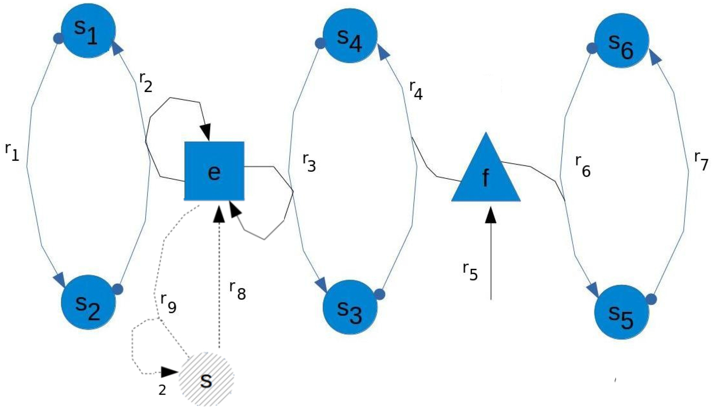
6. Example
In Figure 2, we show an example of a reaction network with species and the reactions:
Let us first consider the set of species . Note that and in X. Moreover, we have with , , and . Hence, we have that a process in is decomposed as , where
For , the minimal fragile-circuit , is weak-self-maintaining if and only if there exists a process such that its non-zero coordinates are all equal. Note that since f is consumed by the weak-self-maintaining processes of the minimal fragile-circuits and , the process that self-maintains X requires that . By Theorem 1, we have that if such processes and exist in the respective restricted process structures , , and , then X is self-maintaining.
In summary, X is self-maintaining if and only if
Consider a process-structure perturbation that leads to a new set of processes , and the possible cases:
- If does not allow Equation (10), X is not self-maintaining, and the set becomes the largest self-maintaining set.
- If does not allow Equation (11), X is not self-maintaining, and the set becomes the largest self-maintaining set. Also, note that is a disconnected set.
- If does not allow Equation (12), X is not self-maintaining, and the set becomes the largest self-maintaining set.
- If does not allow Equation (13), X is not self-maintaining. Moreover, in case , the set becomes the largest self-maintaining set, and in case becomes the largest self-maintaining set inside X, respectively.
We now consider the inclusion of the species s and reactions and as a topology-structure perturbation. Since and consumes and produces the species e, respectively, we have that e is not a catalyst in , and thus the minimal fragile-circuits and merge into a new minimal fragile-circuit in the decomposition of . Thus, .
The analysis of self-maintainance for can be done in an analogous way to the analysis for X by defining the restricted process structure of the minimal fragile-circuit . Note, however, that if does not allow processes such that is not weak-self-maintaining, e.g., when the process vector cannot have equal values for the coordinates representing and , we have that the largest self-maintaining set inside is .
Therefore, we can propose that is more sensitive than X to a process-structure perturbation because the decomposition of X has more minimal fragile-circuits than the decomposition of .
7. Conclusions
We have extended the application of reaction networks, and its COT implementation, as a representational framework for systemic modeling [6]. In this framework, a system corresponds to a sub-network that holds structural properties that ensure its qualitative identity (structurally closed) and observability (self-maintaining), i.e., organizations in the COT sense. Technically speaking, organizations characterize the global invariants of the local dynamics and can be computed at a computationally tractable cost. In particular, we developed a formal framework to study structural changes of a system. A structural change goes beyond the change of state, and encompasses changes that modify the inner functioning rules of the system or the very entities defining the system.
We have introduced the notion of dynamical-connectivity, which explains when two species and are co-dependent for verifying the self-maintenance of a set X that contains them. This notion, which strongly depends on the overproducible species and catalysts, can be applied to maximally decompose the set X into a collection of minimal fragile-circuits, whose weak-self-maintenance implies the self-maintenance of X (Theorem 1). The decomposition Theorem allows for formalizing two types of structural perturbation that extend the notion of perturbation usually applied in the field of dynamical systems: process-structure and topology-structure perturbation. A process-structure perturbation represents a change of the possible processes in the reaction network universe. The topology-structure perturbation represents a change in the reaction network universe itself, i.e., more/less species and/or more/less reactions. We showed how the decomposition allows for precisely identifying the impact of a perturbation. In particular, a perturbation can either affect a minimal fragile-circuit and/or the set of catalysts and overproducible species . When the perturbation affects a minimal fragile-circuit, the analysis of its impact can be studied within the minimal fragile-circuit, while when the perturbation affects , the overall decomposition structure becomes affected. A general perturbation combines effects in some minimal fragile-circuits as well as in . This, in turn, modifies the set of organizations in the perturbed reaction network. Hence, by comparing the sets of organizations before and after the perturbation, we obtain a picture of the effects of the perturbation in the long-term dynamical properties of the system.
We propose that the structural perturbations introduced in this paper, and the analysis of such perturbations under the light of the decomposition Theorem, can be used as a starting point for the formal study of modern systemic dynamical notions such as resilience, adaptivity, robustness, etc. For example, resilience is generally understood as the ability of a system to cope with change. However, this statement is hard to formalize because, since the functioning of a system is understood as a complex process, it is not clear what is a change, or how we identify the part of the system affected by a change, and thus there is no formal framework for defining resilient response-mechanisms. In our framework, we define the notion of structural perturbation that encompass the idea of ‘change’, vaguely defined in resilience literature. Moreover, since we are able to precisely identify the impact of a structural perturbation, we can characterize response mechanisms within the process-structure.
In order to fully develop the mathematical framework to study modern systemic notions, various aspects must be considered. In particular, a deeper characterization of the process-structure and topology-structure perturbations is needed. Such characterization requires combining geometrical properties of the process-structure with structural information of the reaction network. To do so, not only are more theoretical notions needed, but also an algorithmic framework for computing these theoretical notions for moderately large reaction networks.
As a final comment, we believe that the language of reaction networks could provide a powerful formal framework to open up systemic modeling and systemic thinking to the scientific domain.
Acknowledgments
The FONDECYT postdoctoral scholarship 3170122 has supported the first author and the FONDECYT grant 1150229 has supported the second author.
Author Contributions
Both authors contributed equally.
Conflicts of Interest
The authors declare no conflict of interest.
References
- Vemuri, V. Modeling of Complex Systems: An Introduction; Academic Press: New York, NY, USA, 2014. [Google Scholar]
- Strogatz, S.H. Nonlinear Dynamics and Chaos: With Applications to Physics, Biology, Chemistry, and Engineering; Westview Press: Boulder, CO, USA, 2014. [Google Scholar]
- Boccaletti, S.; Grebogi, C.; Lai, Y.C.; Mancini, H.; Maza, D. The control of chaos: Theory and applications. Phys. Rep. 2000, 329, 103–197. [Google Scholar] [CrossRef]
- Maturana, H.R. The organization of the living: A theory of the living organization. Int. J. Man-Mach. Stud. 1975, 7, 313–332. [Google Scholar] [CrossRef]
- Licata, I.; Minati, G. Emergence, computation and the freedom degree loss information principle in complex systems. Found. Sci. 2016. [Google Scholar] [CrossRef]
- Veloz, T.; Razeto-Barry, P. Reaction networks as a language for systemic modeling: Fundamentals and examples. Systems 2017, 5, 11. [Google Scholar] [CrossRef]
- Dittrich, P.; Di Fenizio, P.S. Chemical organisation theory. Bull. Math. Biol. 2007, 69, 1199–1231. [Google Scholar] [CrossRef] [PubMed]
- Peter, S.; Dittrich, P. On the relation between organizations and limit sets in chemical reaction systems. Adv. Complex Syst. 2011, 14, 77–96. [Google Scholar] [CrossRef]
- Peter, S.; Veloz, T.; Dittrich, P. Feasibility of organizations-a refinement of chemical organization theory with application to p systems. In Proceedings of the Eleventh International Conference on Membrane Computing (CMC11), Jena, Germany, 24–27 August 2010; p. 369. [Google Scholar]
- Kreyssig, P.; Wozar, C.; Peter, S.; Veloz, T.; Ibrahim, B.; Dittrich, P. Effects of small particle numbers on long-term behaviour in discrete biochemical systems. Bioinformatics 2014, 30, i475–i481. [Google Scholar] [CrossRef] [PubMed]
- Veloz, T.; Reynaert, B.; Rojas, D.; Dittrich, P. A decomposition Theorem in chemical organizations. In Proceedings of the European Conference in Artificial Life—ECAL, Paris, France, 8–12 August 2011. [Google Scholar]
- Strang, G. Introduction to Linear Algebra; Wellesley-Cambridge Press: Wellesley, MA, USA, 2011. [Google Scholar]
Figure 1.
Note that in (a), the self-maintainance of and are independent because e is a catalyst; The same situation occurs in (b) with sets and with o an overproducible species. Hence, although X is connected (see Definition 2), the potential fragile-circuit can be partitioned into two dynamically-independent sets and .

Figure 2.
Example of a reaction network for showing notions of decomposition, process-structure and topology-structure perturbation. Arrows are labelled by the number of the reaction that they represent, and, at the end of the arrow, the number of produced species by the reaction is shown only when such number is larger than one.


Table 1.
Table of properties associated with a reaction network analysis for a process-structure perturbation.
Table 1.
Table of properties associated with a reaction network analysis for a process-structure perturbation.
| Change | Might Create | Possible Consequence | |
|---|---|---|---|
| Ex. 1 | Larger minimal fragile-circuits | ||
| Ex. 2 | is not weak-SM w.r.t | X is not self-maintaining |
Table 2.
Table of properties associated with reaction network analysis for a topology-structure perturbation. The symbols ⊂ (⊆) and ⊃ (⊇) symbols means that the set referred by the column will become smaller (or equal) and larger (or equal), respectively, after a perturbation. # Min Cyc. stands for number of minimal cycles, and SM stands for self-maintainance.
| Type | X | F | E | C | # Min Cyc. | SM | |
|---|---|---|---|---|---|---|---|
| (i) | ⊂ | ⊂ | ⊆ or ⊇ | ⊆ or ⊇ | ⊆ or ⊇ | More/Less | ? |
| (ii) | = | ⊂ | ⊆ | ⊇ | ⊆ or ⊇ | More/Less | ? |
| (iii) | = | ⊃ | ⊇ | ⊆ | ⊆ or ⊇ | More/Less | ? |
| (iv) | ⊃ | ⊃ | ⊇ | ⊆ or ⊇ | ⊆ or ⊇ | More/Less | ? |
© 2017 by the authors. Licensee MDPI, Basel, Switzerland. This article is an open access article distributed under the terms and conditions of the Creative Commons Attribution (CC BY) license (http://creativecommons.org/licenses/by/4.0/).
Share and Cite
MDPI and ACS Style
Veloz, T.; Razeto-Barry, P. Reaction Networks as a Language for Systemic Modeling: On the Study of Structural Changes. Systems 2017, 5, 30. https://doi.org/10.3390/systems5020030
AMA Style
Veloz T, Razeto-Barry P. Reaction Networks as a Language for Systemic Modeling: On the Study of Structural Changes. Systems. 2017; 5(2):30. https://doi.org/10.3390/systems5020030
Chicago/Turabian StyleVeloz, Tomas, and Pablo Razeto-Barry. 2017. "Reaction Networks as a Language for Systemic Modeling: On the Study of Structural Changes" Systems 5, no. 2: 30. https://doi.org/10.3390/systems5020030
Note that from the first issue of 2016, this journal uses article numbers instead of page numbers. See further details here.