
Ranking of Downstream Fish Passage Designs for a Hydroelectric Project under Spherical Fuzzy Bipolar Soft Framework


1
Department of Mathematics, Division of Science and Technology, University of Education, Lahore 54770, Pakistan
2
Faculty of Science and Technology, University of the Faroe Islands, Vestarabryggja 15, FO 100 Torshavn, Faroe Islands, Denmark
3
Department of Mathematics, College of Science, King Saud University, P.O. Box 22452, Riyadh 11495, Saudi Arabia
*
Author to whom correspondence should be addressed.
Symmetry 2022, 14(10), 2141; https://doi.org/10.3390/sym14102141
Submission received: 8 September 2022
/
Revised: 27 September 2022
/
Accepted: 3 October 2022
/
Published: 13 October 2022
(This article belongs to the Special Issue Algorithms for Multi-Criteria Decision-Making under Uncertainty)
Abstract
:Nowadays, several real-world decision-making problems concerning falling economies, power crises, depleting resources, etc., require efficient decision-making. To solve such problems, researchers proposed several hybrid models by combining the spherical fuzzy sets with other theories, such as spherical fuzzy soft sets, which is an efficient tool to deal with the uncertainties concerning positive, neutral, and negative memberships in the soft environment. However, all the existing hybridizations of spherical fuzzy sets fail to deal with information symmetrically in a bipolar soft environment. Accordingly, this paper presents a novel hybrid model called spherical fuzzy bipolar soft sets (SFBSSs) by fusing spherical fuzzy sets and bipolar soft sets, considering the opposite sets of parameters in symmetry. An example considering the selection of a chief management officer (CMO) for a multi-national company illustrates the proposed model in detail. In addition, some symmetric properties and algebraic operations of the initiated model, including subset, complement, relative null SFBSSs, relative absolute SFBSSs, extended union, extended intersection, restricted union, restricted intersection, AND, and OR operations, are discussed and illustrated via numerical examples. Further, some fundamental results, namely, commutativity, associativity, distribution, and De Morgan’s laws are presented for SFBSSs. Moreover, by considering the massive impact of hydropower in combating the energy crisis and possible dangers to fish migration, a multi-attribute decision-making problem concerning the ranking of downstream fish passage designs for a hydroelectric project is modeled and solved under the developed algorithm based on SFBSSs. Finally, a comparative analysis discusses the supremacy of the initiated model over its building blocks.
1. Introduction
Complicated situations concerning intricate decision-making problems need effective decision-making to handle uncertainties reliably. The decision-making tools and models developed by decision-making scientists and researchers contribute to solving such issues comprehensively and reliably. However, increasing complexities in this field quest for more powerful models with broader approaches and accuracy to handle the emerging uncertainties effectively. Contributing to the solution of uncertain decision-making problems, Zadeh [1] introduced fuzzy set (FS) theory as an effective tool by considering fuzzy memberships depicting the partial truth between the bounds of absolute truth and absolute false (unlike the previous classic theories incapable of translating uncertainties). Advancements based on this theory provided solutions to many uncertain problems but failed to consider parametrization. To mark multiple parameters for decision-making under the same set, Molodtsov [2] proposed the notion of soft sets (SSs) as parameterized families of sets. These sets allow solutions to problems seeking a solution based on multiple parameters. Many hybridizations emerged from these soft sets and offered multi-criterion uncertain decision-making. Among these developments, bipolar soft sets (BSSs) [3] proposed by Shabir and Naz in 2013, provide solutions to the decision-making problems by taking the symmetrically opposite sets of parameters into account. This development allowed solutions to situations where parameters depict bipolarity, such as old and young, good and bad, dull and intelligent, etc. Later, in 2018, Kahraman and Gündogdu [4] introduced spherical fuzzy sets (SFSs) as a powerful extension of fuzzy set theory. These spherical fuzzy sets consider positive, negative, and neutral memberships, reflecting agreement, disagreement, and neutrality in the decision-maker’s opinions, having a much broader scope than the previous models. This quality allowed applications of spherical fuzzy sets in decision-making problems considering surveys, poles, sentiment analyses, etc.
The burning problems of the world such as power generation, depleting resources, shattering economies, environmental hazards, etc., require decision-making tools capable of depicting the naturally occurring bipolarity in the parameters affecting the situations, as well as the consideration of agreement, neutrality, and disagreement of decision-makers for handling the complicated uncertainties. Analogous to this requirement, this research focuses on developing a decision model capable of depicting the bipolarity of parameters in a spherical fuzzy environment. Consequently, it will provide solutions to the complicated decision-making problems unsolvable by the existing theories. The following are the motivations for this work:
Motivated by the aforementioned arguments, the major contributions to this paper are as follows:
- The properties, operations, and results of the proposed model are provided and supported with illustrative examples.
- An algorithm for SFBSSs is provided to deal with MADM problems efficiently.
- A reality-based problem, i.e., the ranking of different downstream fish passage designs for a new hydroelectric project is modeled and solved using the initiated algorithm based on SFBSSs.
The following subsection discusses the literature review related to this work, and the research gaps addressed in this paper.
1.1. Literature Review
Taking a deeper dive into the uncertain decision-making problems followed by the modern probability theory in the 16th century, many researchers have provided a number of decision-making models and algorithms, capable of handling many uncertain problems concerning their respective domains and restrictions. This space of decision-making tools is expanding continuously with the ever-increasing problems as we come to newer and more complex situations needing more powerful tools with broader implementation and applicability. In 1965, a revolution occurred in the decision sciences, when Zadeh [1] came up with his idea of fuzzy sets. This concept for the first time allowed solutions to situations questing for partial truth between the bounds of absolute truth and absolute false, which were unsolvable by previous theories such as the crisp set theory. These fuzzy sets considered membership degrees for elements ranging from 0 to 1 (belonging to the closed interval ), rather than the discrete values 0 and 1, thus providing a better insight into how much something belongs, instead of only declaring whether it belongs or not. Later, this idea was applied and further improved by many decision-makers over the globe.
A limitation of the above-discussed fuzzy sets is their inefficiency in considering a relatively independent degree of dissatisfaction, that is, they do not consider the non-membership degrees. Atanassov [11] filled this gap by introducing the intuitionistic fuzzy sets (IFSs), which considered both membership degrees and non-membership degrees of the elements with the condition that their mutual sum must not exceed unity. Later, Atanassov [12] extended the same to a more applicable form, i.e., the ‘IFSs of second type’ by smoothening the mutual sum condition as he restricted the sums of squares of the two memberships to unity. In 2013, Yager [13] introduced Pythagorean fuzzy sets identical to Atanassov’s IFSs of second type. This generalized version of the IFSs showed relatively more applicability in comparison with the previous models [14,15,16,17]. Recently, Hayat et al. [18] introduced new aggregation operators for group generalized q-rung orthopair fuzzy soft sets and discussed their decision-making applications. Naz et al. [19] evaluated network security service providers using 2-tuple linguistic complex q-rung orthopair fuzzy COPRAS method.
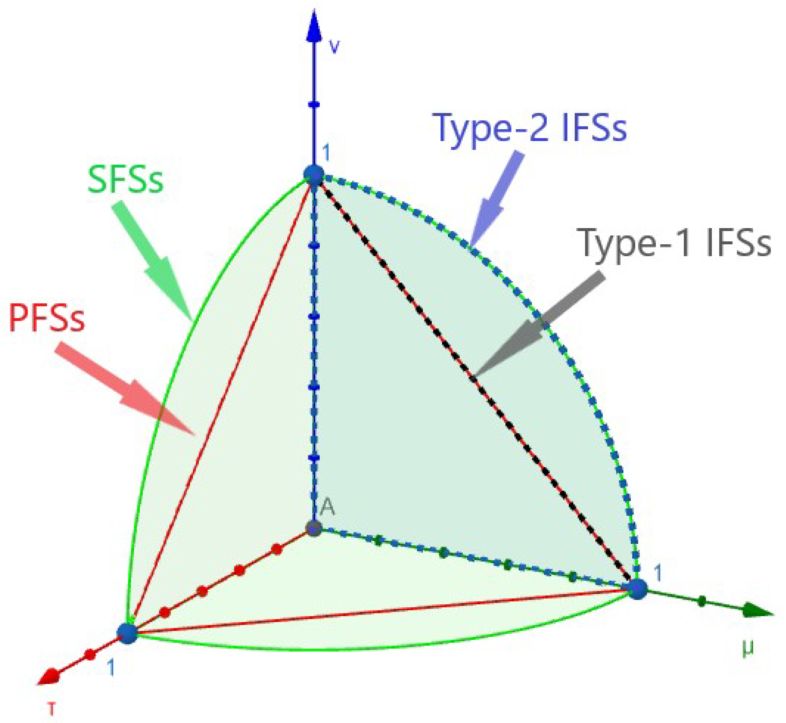
Despite their efficiency, the aforementioned models fail to depict the neutrality of opinions, that is, they cannot be helpful in problems concerning neutral membership degrees. For instance, in an election, a voter’s opinion may be neutral, satisfactory or dissatisfactory for a candidate. In such cases, a degree of neutrality is also needed for better demonstration. To tackle this issue, picture fuzzy sets (PFSs) were introduced by Coung [5,6]. These PFSs considered neutral membership in addition to the positive membership and negative membership of the element , subject to the constraint . This concept proved its importance in many problems concerning neutral opinion as in the case of sentiment analysis, surveys, poles, etc. Wei [20,21] provided similarity measures for picture fuzzy sets. Karamti et al. [22] applied PFSs for evaluating pedagogic systems to enhance the e-learning system. Recently, Singh and Ganie [23] provided the application of picture fuzzy correlation coefficient in pattern analysis. These sets prove to be a very powerful decision-making tool but fail to consider the scenarios where the sum of the membership, nonmembership and neutral degrees exceeds unity. To deal with this difficulty, Kahraman and Gündogdu [4] introduced the spherical fuzzy sets (SFSs) where the membership, nonmembership and neutral degrees are restricted by the condition . Figure 1 represents the IFSs(Type-1 and Type-2), PFSs, and SFSs, pictorially to represent their applicable domains. In 2019, Gündogdu and Kahraman [24] proposed generalized SFSs and provided a technique of order preference similarity to the ideal solution (TOPSIS)-based decision application of SFSs. Akram et al. [25] assessed the hydropower plants in Pakistan under Muirhead mean-based 2-tuple linguistic T-spherical fuzzy model. In recent years, many researchers have used SFSs to deal with decision-making problems [26,27,28,29,30].
All the above-discussed models lack parameterization and therefore are not very helpful in situations concerning decisions respective to multiple parameters. In this regard, Molodtsov [2] firstly initiated the concept of soft sets as a parameterized family of sets. Maji et al. [31] provided the applications of soft sets in decision-making. This concept proved its applicability in a huge number of problems from all fields of science including humanity, medicine, economics, artificial intelligence, and so on. Many decision-makers combined previously existing models with soft sets to make powerful hybrid MADM models. Perveen et al. [7] introduced spherical fuzzy soft sets (or SFSSs) and their application in the MADM problem. In 2020, Hayat et al. [32] evaluated design concepts using soft sets by considering the integrated TOPSIS and Shannon entropy methods. Hayat et al. [33] proposed aggregation operators for group-based generalized intuitionistic fuzzy soft sets. Guleria and Bajaj [34] proposed T-SFSSs. Akram et al. [35] introduced complex spherical fuzzy N-soft sets and their applications. In addition, Akram et al. [36] proposed spherical fuzzy N-soft sets and discussed its survey-based applications.
Many times in daily decision-making problems, the decision-makers come across situations considering the bipolarity, or the two-sided conditions, where one parameter symmetrically affects the other one. The above-mentioned models are incapable of dealing with the two-sided information in a soft environment, such as the inter-effective parameters as bright and dark, hot and cold, old and young, where one side is contrary to the other side. To deal with such kind of situations, Shabir and Naz [3] introduced the concept of bipolar soft sets (BSSs), where two oppositely meaning sets of parameters namely the “set of parameters” and the “not set of parameters” are considered in symmetry with each other. Hence, this model deals with the bipolarity of soft data more efficiently than its predecessors. Later, Naz and Shabir [10] combined their BSSs with fuzzy sets to develop fuzzy BSSs. Ali et al. [37] introduced bipolar soft expert sets as a combination of BSSs and soft expert sets. Ali and Ansari [8] developed Fermatean fuzzy BSSs. Later, Ali et al. [38] introduced fuzzy bipolar soft expert sets and ranked the Coronavirus Disease 2019 tests. Some other BSSs-based hybrid structures have also been presented in recent years [9,39].
The SFS-based models are incapable of translating the bipolar behavior of parameters, whereas the BSS-based models fail to consider the degrees of agreement, neutrality, and disagreement in a decision-making problem. To fill these gaps in the existing theories, this research work provides a new model as a generalization of the aforementioned models that not only fills these gaps but also combines the properties of existing models in a reliable way. Consequently, this new approach offers more generalized and accurate solutions to complicated problems by taking the maximum considerations into account, as indicated by Table 1.
1.2. Organization
The organization of the paper is provided as follows: Section 2 provides the preliminary definitions and results. Section 3 introduces a novel hybrid model namely, SFBSSs along with its basic operations and properties. Section 4 provides an algorithm for solving MADM problems with SFBSSs and explores a daily life ranking application concerning fish passage designs for a new hydropower project. Section 5 discusses advantages, limitations, and a comparative analysis of the proposed model with some existing models. Finally, Section 6 shows the conclusive remarks and the future considerations respective to the proposed work.
2. Preliminaries
This section revises some definitions and properties, which will be helpful in the study of upcoming sections. The following recalls the definition of spherical fuzzy sets [4], which acts as a basic unit for the newly developed hybrid model in the next section.
Definition 1
([4]). A spherical fuzzy set (or SFS) over the universe is defined as:
such that , and represent the positive, neutral, and negative membership degrees of , respectively, restricted to the constraint
The collection of all SFSs on is denoted by .
Considering SFSs as the basic unit, the properties and operations of the developed model will be based on the following properties of SFSs:
Definition 2
([4]). Let and be two SFSs over the universe , then:
- 1.
- if , and
- 2.
- ⇔ and
- 3.
- 4. .
- 5. .
The notion of spherical fuzzy soft sets (or SFSSs) is provided below:
Definition 3
([7]). For representing the set of parameters, the universe of objects, and , the set is said to be a spherical fuzzy soft set (SFSS) over the universe , where and , the function is defined as
such that and represent the positive, neutral, and negative membership degrees of , respectively, restricted to the constraint
The following definitions recall the level sets and threshold functions for SFSSs, which will be used in the development of the decision-making algorithm for the proposed model.
Definition 4
([7]). For being a SFSS over the universe , consider the function , such that , with and belonging to the interval . Then, the level soft set of Υ corresponding to the function λ gives a crisp set defined as:
Definition 5
([7]). For being the SFSS over , the four renowned threshold functions are defined as follows:
- 1.
- Mid-level Threshold Function ():The function for the SFSS is given bysuch thatandThe mid-level soft set of Υ under is denoted by .
- 2.
- Top-bottom-bottom-level Threshold Function ():The function for the SFSS is given bysuch thatThe tbb-level soft set of Υ under is denoted by .
- 3.
- Bottom-bottom-bottom-level Threshold Function ():The function for the SFSS is given bysuch thatThe bbb-level soft set of Υ under is denoted by .
- 4.
- Med-level Threshold Function ():The function for the SFSS is given bysuch thatHere, and represent the medians calculated by ranking the positive, neutral and negative membership degrees, respectively, in ascending (or descending) orders. The med-level soft set of Υ under is denoted by .
Now, we recall the definition of bipolar soft sets.
Definition 6
([3]). For being the universe, and being the set of parameters, the triple is called a bipolar soft set (BSS) over for some , if the mappings ζ and ψ are defined, respectively, as:
Here, represents the not-set of containing the parameters opposite to those contained in , such that
with representing the power set of .
3. Spherical Fuzzy Bipolar Soft Sets
This section introduces the novel hybrid model, namely spherical fuzzy bipolar soft sets (SFBSSs), and discusses its properties and operations with illustrative examples. Based on BSSs and SFSs, the novel SFBSSs are defined as follows:
Definition 7.
For being the universe of objects, and being the universe of parameters related to the objects in , a triple is said to be a spherical fuzzy bipolar soft set (SFBSS), if for , the mappings ζ and η are defined, respectively, as:
Here, represents the not-set of containing the parameters opposite to those contained in , whereas represents the collection of all spherical fuzzy sets defined on .
For all and ,
where μ, τ, and ν are positive, neutral and negative membership degrees, respectively, such that , the following conditions hold:
The following example gives an illustration of the modeling of decision-making problems using SFBSSs.
Example 1.
Consider a multi-national company with lots of products and services globally, loses its CMO (Chief Marketing Officer) due to some reasons, and now needs to assign a new CMO in order to dominate and survive the competition with its marketing rivals. However, choosing the best CMO in order to maximize profit and dominance is a difficult task. To overcome this issue, the company owner hires a very effective marketing expert to choose the best candidate from one of the few available options.
Consider there were five candidates for the post, out of which only three are shortlisted on the basis of their basic qualifications, that is, academics and experiences. The shortlisted candidates comprise the set . Suppose that the consulted expert considers the set as the set of key-parameters, and satisfying it is considered the key to the post. On the other hand, the set , is considered as the set of non-favorable decision-parameters, while considering the post for the CMO.
After analyzing the candidates, the expert makes the report in form of an SFBSS as follows:
Table 2 and Table 3 give the tabular representation of the above SFBSS in terms of ζ and η, where and are SFSSs.
The single table representation for the above SFBSS is given in Table 4, whereas Table 5 represents the generalized single table form for SFBSSs.
From here, it can be clearly observed that the expert considers more diverse in his skills as compared to the other candidates, whereas is declared as the most unpretentious person, and so on.
The following definition gives the subset relation between two SFBSSs.
Definition 8.
an SFBSS is said to be a subset of another SFBSS , if the following conditions hold:
- 1.
- 2.
- and and
- 3. .
- and and
This subset relation is denoted as . Similarly, Ψ is said to be the superset of Ξ denoted as .
Example 2.
Reconsider Example 1. Let and . Clearly .
Here or .
Definition 9.
Any two SFBSSs Ξ and Ψ are said to be equal SFBSSs if they are both spherical fuzzy bipolar soft subsets of each other. That is,
Based on SFS complement, the following definition introduces the complement of an SFBSS.
Definition 10.
The complement of SFBSS is another SFBSS given by , such that and , and are mappings, respectively, defined as:
Example 3.
Reconsider the SFBSS in Example 1. Using Definition 10, its SFBS complement, i.e., is represented in Table 8.
Proposition 1.
Let be an SFBSS on , then
- 1.
Proof.
- 1.
- From Definition 10, we have such thatThis implies thatHence, , or
□
Definitions 11 and 12 introduce the concepts of relative null and relative absolute SFBSSs.
Definition 11.
An SFBSS is said to be a relative null SFBSS over , if ,
and ,
Definition 12.
An SFBSS is said to be a relative absolute SFBSS over , if ,
and ,
The AND operation between two SFBSSs is defined as follows:
Definition 13.
For two SFBSSs and over the universe , the AND operation between them is represented by an SFBSS defined as
such that and , and are mappings, respectively, defined as:
The OR operation between two SFBSSs is defined in the following definition.
Definition 14.
For two SFBSSs and over the universe , the OR operation between them is represented by an SFBSS defined as
such that and , and are mappings, respectively, defined as:
The following gives an example of the AND and OR operation between two SFBSSs.
Example 4.
Proposition 2.
Let and be two SFBSSs on , then
- 1.
- 2.
Proof.
- 1.
- Let . Then, for all ,whereand .Now consider for allwhere , and .Clearly, we have and . Hence .
- 2.
- Let . Then for all ,whereand .Now consider for allwhere andClearly, we have and . Hence .
□
Proposition 3.
Let and be three SFBSSs over , then
- 1.
- 2.
- 3.
- 4.
Proof.
- 1.
- By Definition 13, we haveHence proved.
- 2.
- By Definition 14, we haveHence proved.
The remaining parts (3) and (4) are immediately followed by similar arguments as discussed in parts (1) and (2). □
Definitions 15 and 16 discuss the restricted intersection and restricted union between two SFBSSs, respectively.
Definition 15.
The spherical fuzzy bipolar soft restricted intersection between the two SFBSSs and is represented by an SFBSS defined as
such that , the mappings and are defined, respectively, as:
where
Definition 16.
The spherical fuzzy bipolar soft restricted union between the two SFBSSs and is represented by an SFBSS defined as
such that , the mappings and are defined, respectively, as:
where
Example 5.
Referring back to Example 1, and considering and ; the corresponding SFBSSs and are represented in Table 13 and Table 14, respectively.
Let . Then, by Definition 15, the restricted SFBS intersection is calculated as shown in Table 15.
Similarly, by using Definition 16, the restricted SFBS union is represented in Table 16.
Proposition 4.
Let , and be two SFBSSs over , then
- 1.
- 2.
Proof.
Straightforward. □
Proposition 5.
Let and be three SFBSSs over , then
- 1.
- 2.
- 3.
- 4.
Proof.
- 1.
- By Definition 15, for all we haveHence proved.
- 2.
- By Definition 16, for all we haveHence proved.
The remaining parts (3) and (4) are immediately followed by similar arguments as discussed in parts (1) and (2). □
Proposition 6.
Let and be two SFBSSs on , then
- 1.
- 2.
Proof.
- 1.
- Let . Then for all ,whereand .Now consider for allwhere andClearly, we have and . Hence .
- 2.
- Let . Then for all ,whereand .Now consider for allwhere andClearly, we have and . Hence .
□
The following two Definitions 17 and 18 give the extended intersection and extended union, respectively, between two SFBSSs, as follows.
Definition 17.
The spherical fuzzy bipolar soft extended intersection between the two SFBSSs and is represented by an SFBSS defined as
such that , the mappings and are defined, respectively, as:
Definition 18.
The spherical fuzzy bipolar soft extended union between the two SFBSSs and is represented by an SFBSS defined as
such that , the mappings and are defined, respectively, as:
Example 6.
Consider the SFBSSs and in Example 5, and suppose that . Then, by using Definition 17, the extended SFBS intersection is shown in Table 17.
Likewise, by using Definition 18, the extended SFBS union is calculated as shown in Table 18.
Proposition 7.
Let , and be three SFBSSs over , then
- 1.
- 2.
- 3.
- 4.
- 5.
- 6.
Proof.
- 1.
- Let . By Definition 17, we have
Eliminating the trivial cases, we are left with the case when , then we have
Similarly,
This implies that . Hence it proves that .
The remaining parts can be proved similarly. □
Proposition 8.
Let and be two SFBSSs over , then
- 1.
- 2.
- 3.
- 4.
- 5.
Proof.
Straightforward. □
4. Application of SFBSSs in MADM Problem
In this section, an algorithm based on the initiated SFBSSs is proposed and implemented in solving an illustrative MADM problem considering the downstream fish passages at hydroelectric projects. A few things need to be discussed as follows, before moving to the application.
Definition 19.
For a triple representing the SFBSS over , the corresponding SFSSs and are said to be the favor SFSS and non-favor SFSS, respectively.
Definition 20.
For level favor soft set and level non-favor soft set calculated by using Definition 4 with entries and , respectively, in tabular form, the corresponding focus-level table consists of the entries , such that
The column sum of these entries gives the focus-level(FL) scores corresponding to the alternatives
Now, we define Algorithm 1 for ranking alternatives based on SFBSSs as follows:
| Algorithm 1: Ranking alternatives under SFBSSs environment |
Output: corresponding to s found in step 8 is the best alternative. For ascending values of s, corresponding s in ascending orders give the required ranking of alternatives. |
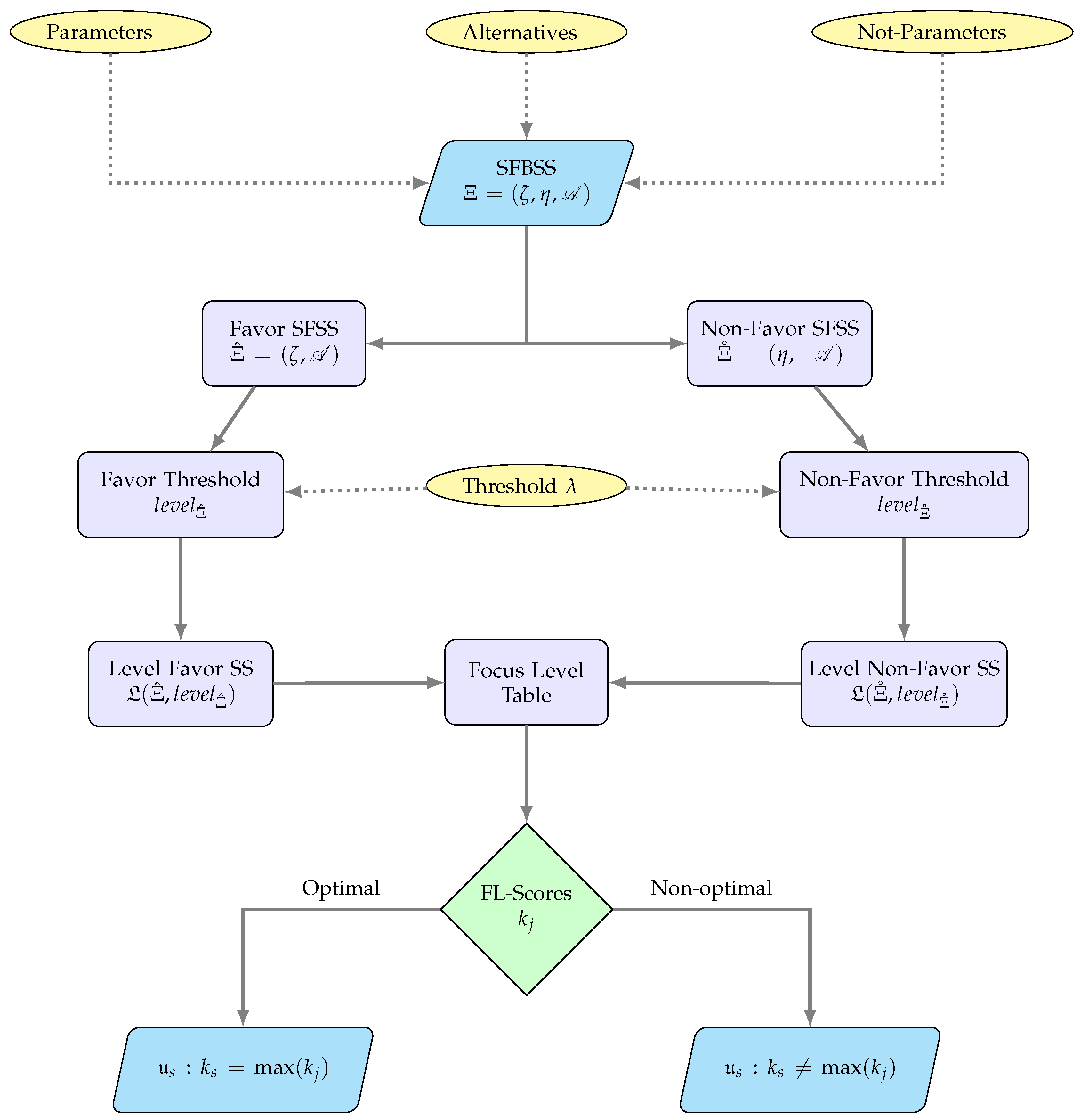
A symmetric flowchart for the above proposed Algorithm 1 is represented in Figure 2.
Example 7.
Ranking of downstream fish-ways designs for a hydroelectric project:
The energy crisis is one of the most pressing issues of our time. With global energy demands increasing every year and pollution levels reaching record highs, a sustainable solution is obviously needed. One of the most promising solutions to this issue is renewable energy. Renewable energy is energy coming from natural sources that are never depleted, such as the sun, wind, earth, and water.
There are many different forms of renewable energy resources with their own pros and cons over each other depending on the overall power generation, initial infrastructure costs, sustainability, maintenance, demographic requirement and ecological and environmental constraints. The major forms include solar power, wind power, hydroelectric power, geothermal energy, and biomass energy (not considering nuclear energy at the moment).
Solar power is one of the most promising renewable energy sources available today. It has the potential to provide clean, efficient energy for homes, businesses, and even entire communities. Solar power is also cost-effective and easy to maintain, making it a very attractive option for those looking to reduce their carbon footprint. Despite its many benefits, solar power still has some limitations. For example, it only works during the daytime, and weather conditions can affect its output. Though improvements are in progress to boost the efficiency of this natural resource.
Another important and widely accepted renewable resource is wind power. Not only is wind power environment-friendly, but it is also very efficient. According to the U.S. Department of Energy, wind power is capable of meeting 10% of the world’s energy needs by 2050. The cost of generating electricity with wind power has also decreased in recent years, making it an even more attractive option for some people. The reason for this drop in price is largely due to improvements made to the technology that produces and transfers electricity from turbines. The main drawback is sustainability as it depends on wind.
Geothermal energy comes from the heat of the earth’s core, which can be harnessed to generate electricity or to heat buildings. Geothermal energy is a clean and renewable resource that does not produce emissions, making it a great choice for those who are looking to reduce their carbon footprint. Plus, geothermal energy is a reliable source of power that can provide electricity even when the sun is not shining or the wind is not blowing. However, there are some drawbacks to this form of energy. It is an expensive form of renewable energy (largely because drilling into the ground to extract heat costs money), so the initial investment may be too high for some people. Geothermal energy also has a low efficiency rate (around 10%), so it can take quite a lot of time before one dollar invested generates $1 worth of power. Moreover, only the areas geologically consistent with this natural resource can benefit from it considering the transmission issues and low efficiency.
Biomass energy is produced from organic materials, such as plants and animals. Biomass energy is also relatively low-cost and efficient. Additionally, biomass energy can be used to produce electricity, heat, and transportation fuels. Biomass can even be converted into chemicals, fibers, and fertilizers. There are many different types of biomass energy sources including cornstalks, peat mosses, bark and algae. All these sources have their own pros and cons depending on where they come from and how they are processed. Some have high costs associated with processing while others may not have enough material available to create any significant amount of fuel at all.
The most sustainable and the most implemented of the renewables is hydroelectric power. Dams and turbines are used to generate hydroelectric power. Tidal energy is also a form of hydroelectric power. Wave and ocean current energy, tidal currents, and ocean thermal gradients all can be harnessed to produce electricity. In the process, they do not release any greenhouse gases into the atmosphere, nor do they contribute to acid rain or smog or other pollution problems. Hydroelectric power provides clean electricity without releasing harmful chemicals into the air or water supply. There are different types of hydroelectric power plants such as pumped storage facilities and run-of-the-river plants. One major benefit of this type of plant is that there is no need for fossil fuels which means less pollutants in the environment. Though it takes time and huge initial costs to set the projects for this form of energy, and countries such as Saudi Arabia with the least water resources are not capable to benefit from this resource efficiently; yet, this is the most adapted and implemented with more than half of the overall renewable energy generated globally by hydroelectric power.
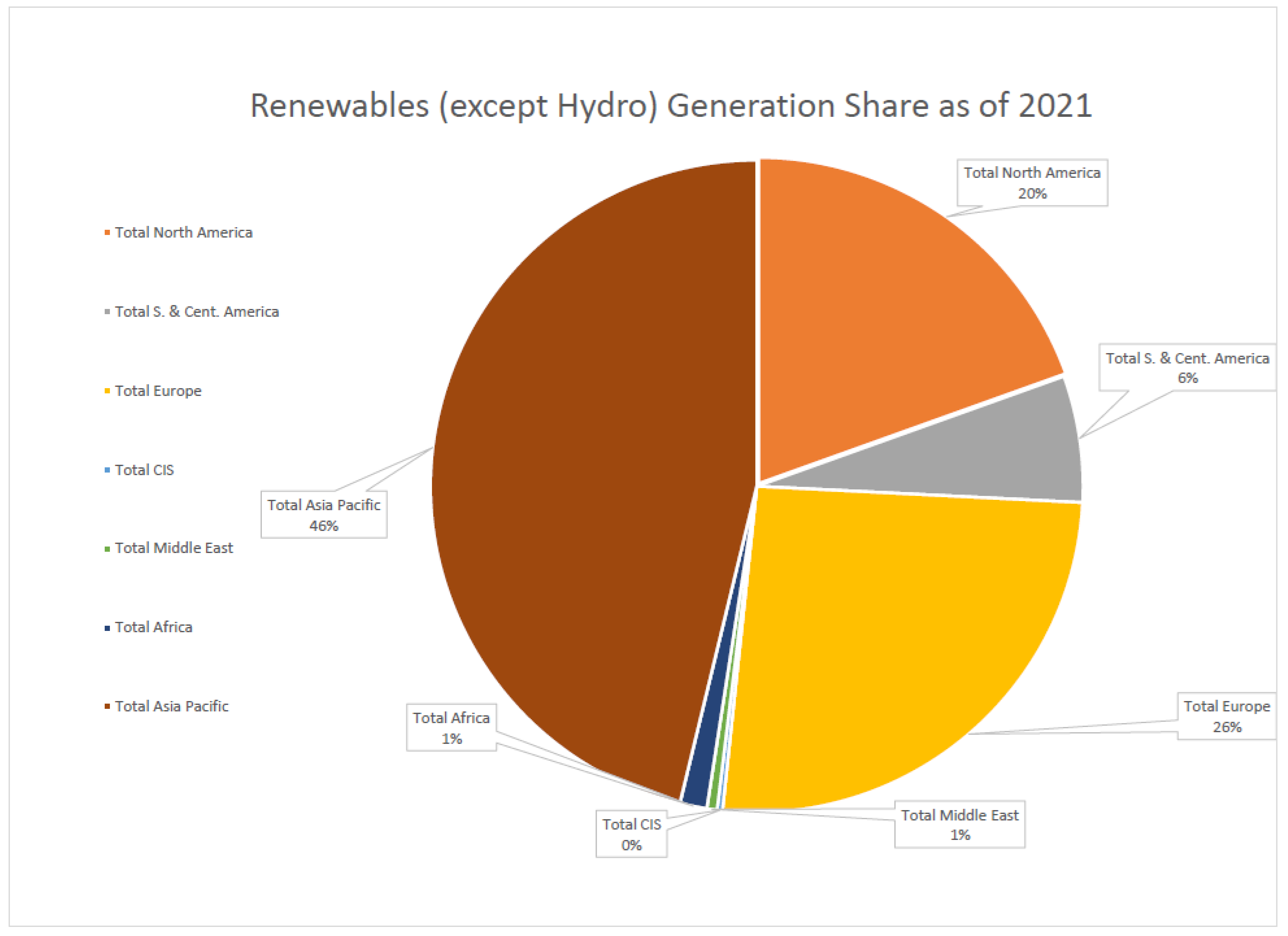
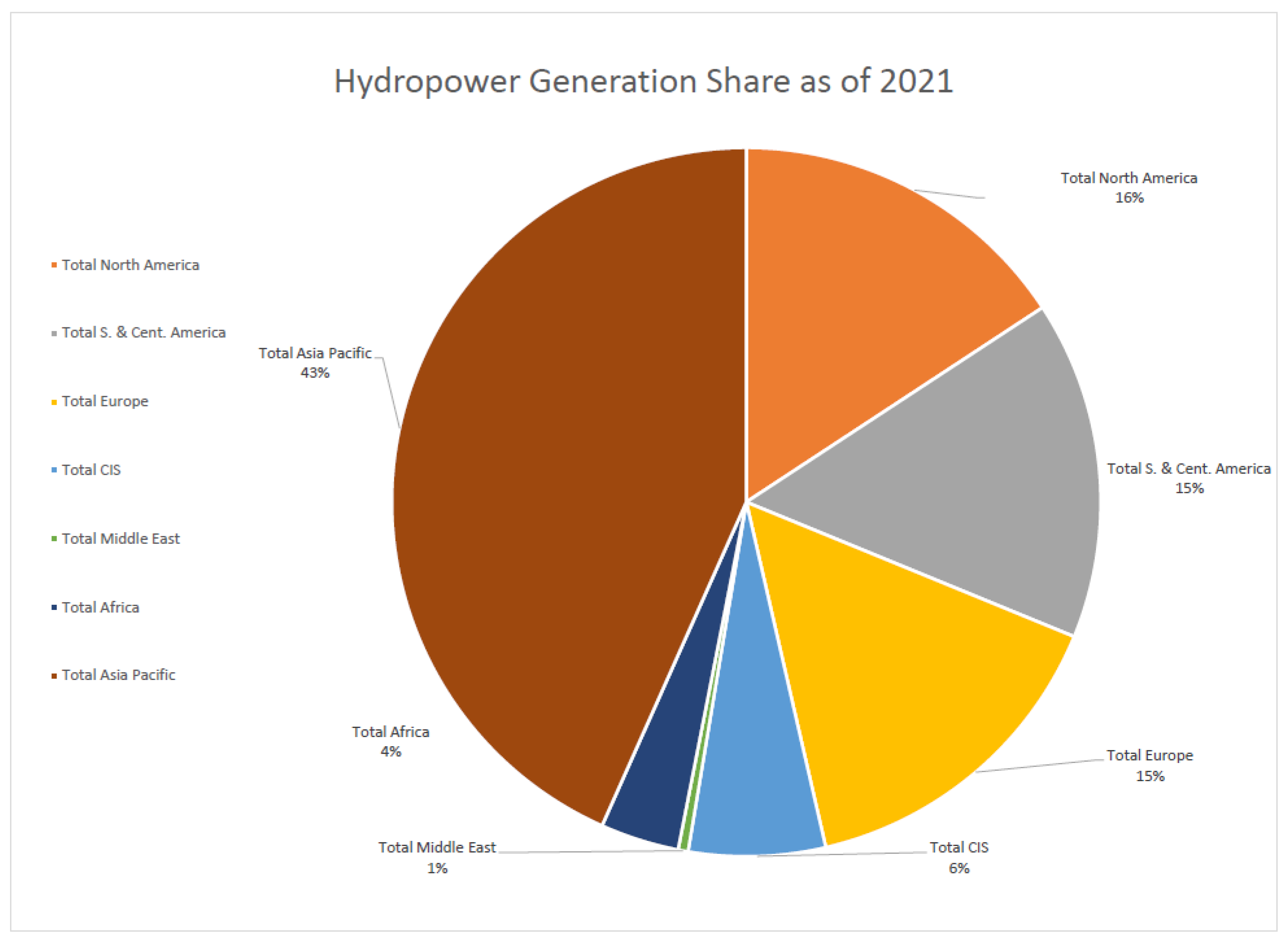
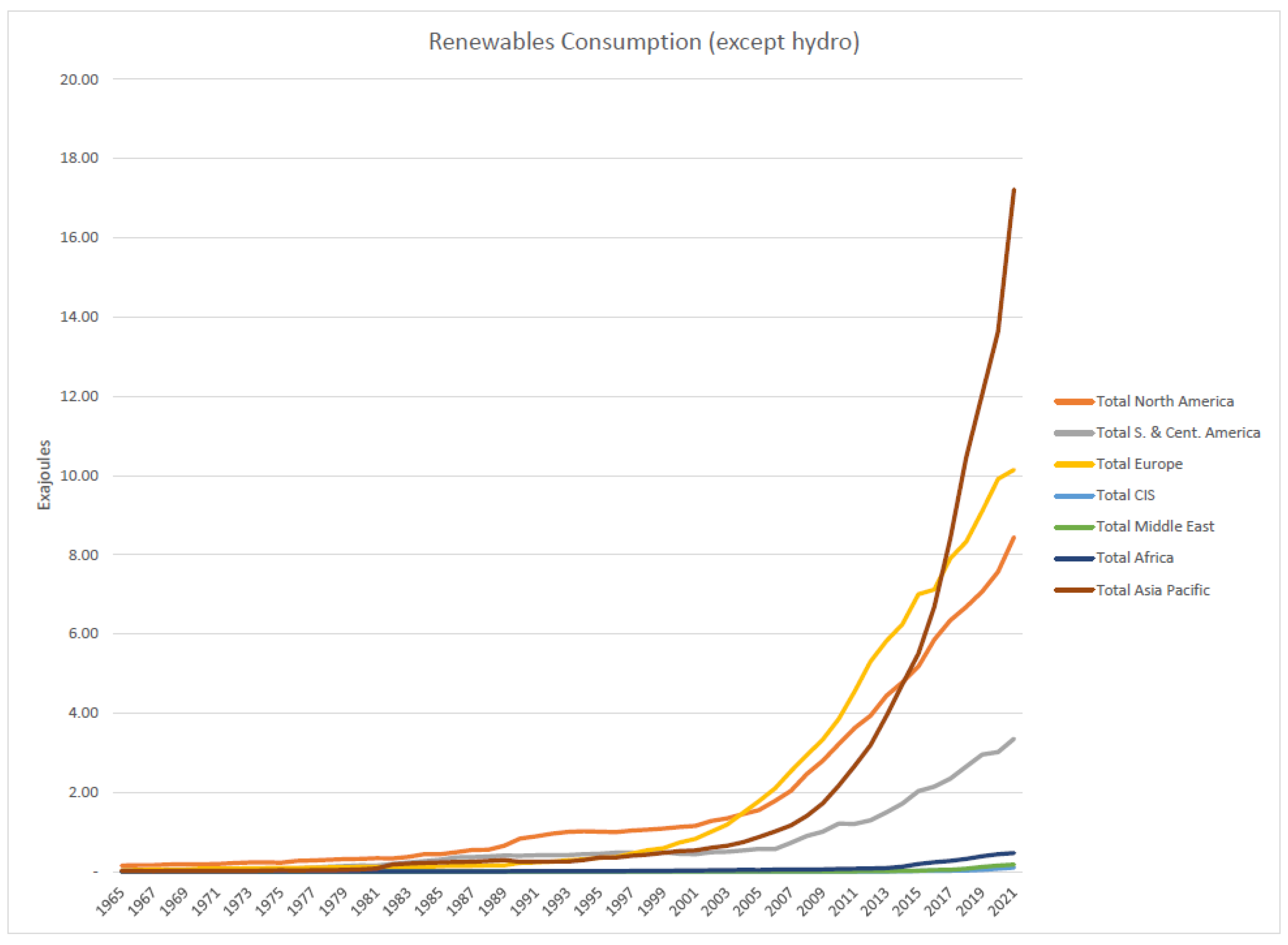
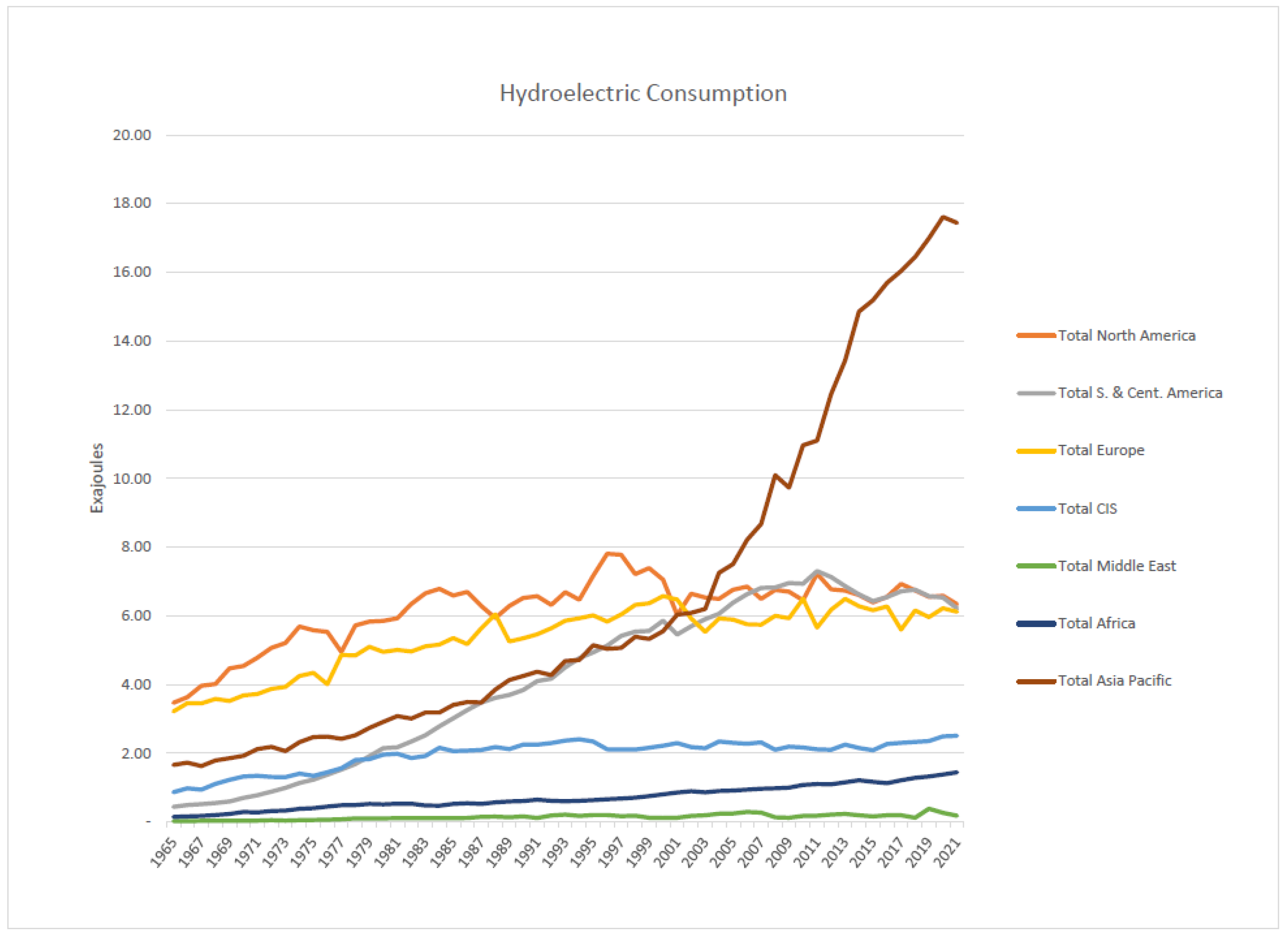
An overall dominance of hydroelectric power over other renewable resources can be seen from the global stats about the consumption and generation of renewable resources. Figure 3 and Figure 4 represent the global share of world’s demographies in generation (https://www.bp.com) (accesssed on 4 August 2022) of renewable resources (except hydropower) and generation of hydropower, respectively. Figure 5 and Figure 6 represent the global increase in consumption of renewable resources with the passage of time. An almost equal amount of hydropower generation and consumption as compared to the remaining renewables can be observed, with the Asia Pacific region dominating others.
Considering these, hydropower is indeed the highest sharing participant in the race of renewables (however, the adaption of solar power is increasing rapidly). Despite the high sustainability, negligible carbon footprint and massive generation, there are challenges in the development of hydropower projects considering many economic, demographic and environmental issues. A hydropower project particularly in the form of a dam is a huge project affecting a large area and the habitat in that area. In the case of dams built on land, they may affect the agricultural patches and communities. Similarly, in rivers, lakes and oceans, one of the important considerations is the fish. Fishes swim in the water and are highly likely to get injured or die due to the turbines, spillways and structures in the dam. Further, dams alter the natural flow, hence concentrating the flux towards them. Fishes cannot be restricted from passing through these structures due to their natural conditions and need of migrating from one place to another in order to spawn, reproduce and continue their growth cycle; restricting this can cause major ecological disturbances. For this reason, fish need to migrate from both upstream and downstream through these dams. Upstream fish passages are passages particularly designed for fish in the form of fish ladders, fish cannons, pumps, lifts and transportation to move the fish from one side to another. On the other hand, downstream fish passages are more complex and relatively controversial for the fish but are also a need for ecological equilibrium. Downstream fish passages require many things to be considered including the fish-friendly turbines, physical barriers, fish guidance components, assisting technologies and behavioral devices such as electric fields, mercury lights, etc., specific to the site and fish species.
In this problem, we consider a new hydropower project to be set on a new site. The main focus will be on the ranking of different designs for the project considering the downstream fish passages, such that fish can migrate safely to the other side. Consider that the data about the site and fish species in the site are gathered thoroughly in order to make the best measures for eco-friendly hydropower generation. Four downstream fishway designs constituting the set are proposed for the project to the permitting committee. The committee considers the set of parameters as favorable parameters, where:
- Safe fish passage ensuring that fishes are able to pass through the passage without injury.
- Economic ensuring that the design will be low-cost and will not make a negative economic impact on the project.
- Good fish guidance considering the effectiveness of measures such as angled bars, racks and walls in guiding the fishes towards passage.
- Effective complementing technology considering the aiding components such as bypass chutes for the procedure.
- Behavioral consistency, ensuring that the design is highly consistent with the species behavior including the swimming velocity, clustering and size.
- Good behavioral guidance considering the alternative behavioral guidance aids such as underwater lights, pulses, etc., to direct the fish through the passage.
In symmetry with the set of parameters , the set represents the not-set of parameters, where
- Fish injury and mortality.
- High cost.
- Bad fish guidance.
- No complementing aids.
- Behavioral inconsistence.
- Bad behavioral guidance.
Based on the models and simulation techniques, the committee generates a collective report in the form of an SFBSS for these designs in Table 19 as shown below:
The permitting committee decides to rank the alternatives using Algorithm 1. The mid-level threshold is considered for decision-making, and thereafter, mid-level favor thresholds and mid-level non-favor thresholds are calculated as:
Corresponding to these thresholds, the mid-level favor soft set and mid-level non-favor soft set are represented in Table 20 and Table 21, respectively.
Now, using the mid-level favor soft set and mid-level non-favor soft set, the focus mid-level scores are calculated in Table 22 as shown below:
The last row indicating the FL-scores shows that is the best design. Based on these final FL-scores, the committee ranks the designs as
However, it can be clearly observed from the report that is also the most expensive design. This means that in the case of a low budget, may be considered by compromising the overall qualities for meeting the cost.
5. Comparison and Discussion
This section discusses the comparison of SFBSSs with respect to previously existing models, the advantages of the proposed model, and the limitations in making decisions with SFBSSs.
5.1. Advantages
With the passage of time and ever-increasing complications in decision-making problems, the need for better and improved tools (and models) is continuously increasing. Researchers around the globe are trying to find solutions to numerous decision-making problems considering the development of models specific to particular constraints and conditions. In this struggle, hybridization of the existing models and tools proves to be very effective in providing broader applicability as well as newer possibilities for the solutions of decision-making problems. Among these hybrid structures, SFSSs [7] have proved their efficiency in discussing MADM problems taking the degrees of agreement, disagreement, and neutrality into account. However, in problems affected by the bipolarity of decision parameters, SFSSs fail to characterize and represent this bipolarity symmetrically. On the other hand, FBSSs [10] are capable of discussing the bipolarity of parameters with ease in a fuzzy environment. Still, FBSSs are not as efficient as SFSSs when concerning uncertainties, as they are restricted to the degrees of memberships only. Our proposed model, i.e., SFBSSs as a generalization of FBSSs and SFSSs not only combines the strengths and properties of these models but also fills the gaps discussed above. As a result, the proposed model can handle the bipolarity of parameters, while considering opinions in the form of positive, negative and neutral membership degrees. Hence, the proposed model allows better handling of MADM problems in comparison with the previous models.
5.2. Comparison
In handling decision-making situations, both SFSSs and FBSSs prove to be very important in their respective domains. However, both of these models have limitations. The SFSSs fail to handle the bipolarity of the decision parameters, whereas FBSSs are not capable to deal with spherical fuzzy information. In this way, SFSSs ignore the bipolarity, whereas FBSSs do not take disagreement and neutrality into consideration. The newly initiated SFBSSs not only have the properties of SFSSs and FBSSs but are also free of the constraints and illegibilities of their base models.
Based on the scores calculated for Example 7 by:
- reducing the SFBSS to FBSS by dropping the neutral and negative membership degrees, and then finding the focus level set as the difference of fuzzy soft sets for the two sets of parameters;
- reducing the SFBSS to SFSS by ignoring the not-set of parameters (and corresponding opinions), and then finding the mid-level SS (in the place of focus set in Algorithm 1.
Table 23 and Table 24 give the comparison of scores, and ranking orders for Example 7 obtained by FBSSs [10], SFSSs [7], and the proposed SFBSSs, respectively.
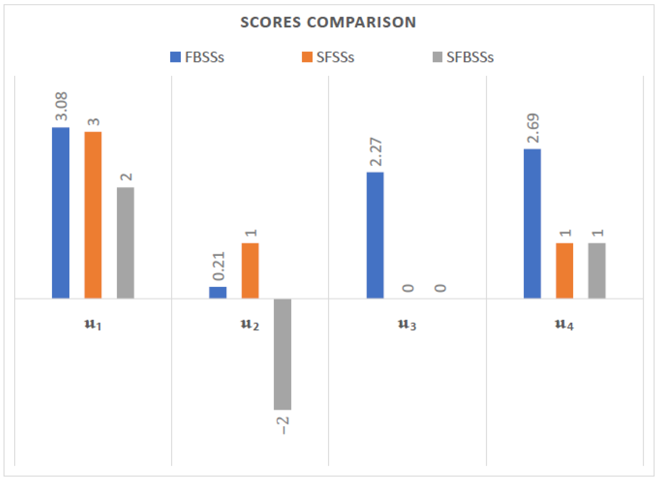
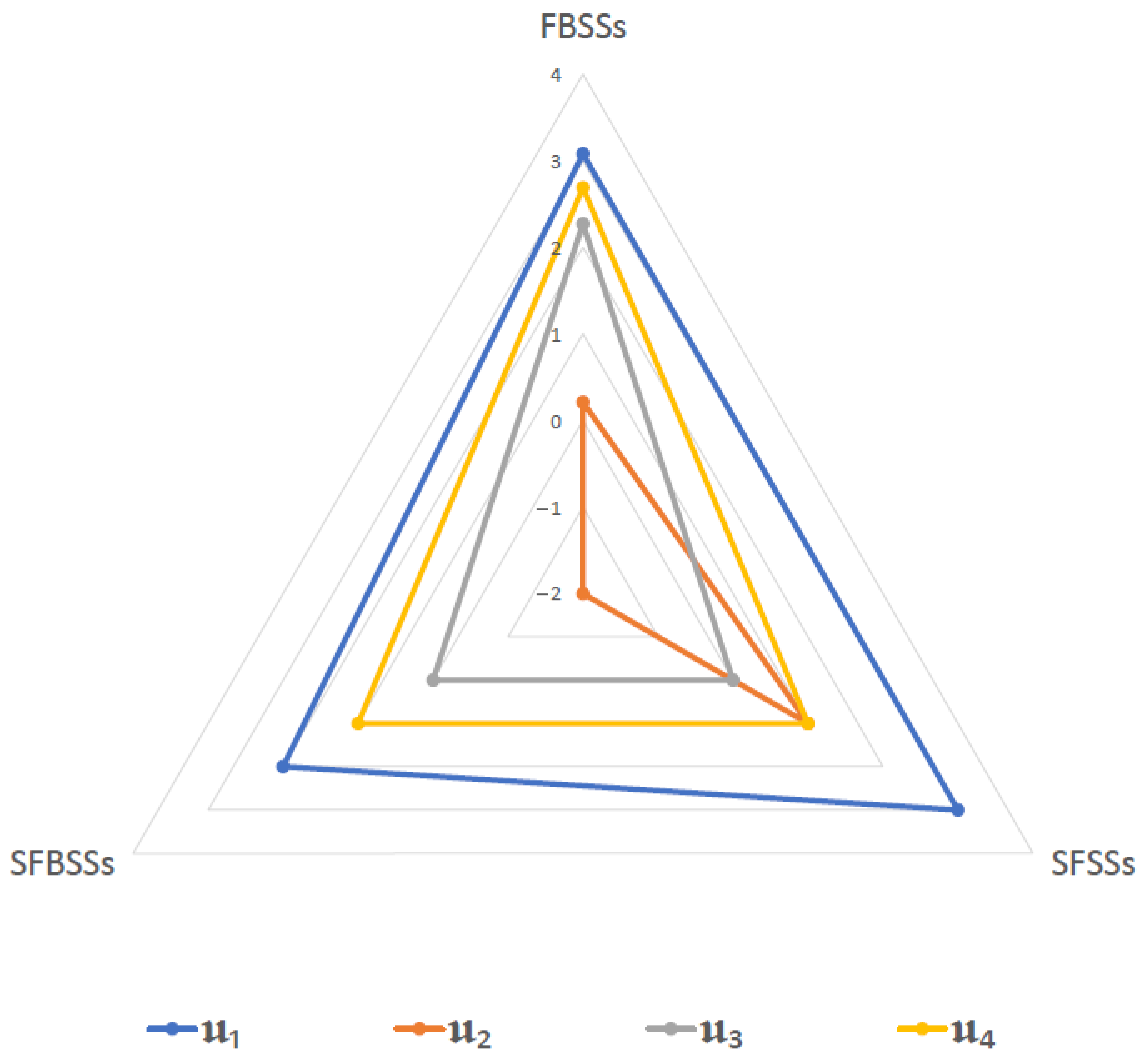
It can be observed that SFSSs fail to provide a distinction between the ranks of and , and hence, cannot provide a clear ranking between the alternatives. Figure 7 gives an alternative-wise comparison indicating the identical scores given by SFSSs and SFBSSs for and . In addition, Figure 8 shows that despite the same rankings generated by FBSSs and SFBSSs, there is an elevation in the final scores for FBSSs due to the absence of degrees of neutrality and disagreement. Thus, for relatively higher values of negative and neutral degrees of memberships, a clear distinction might be observed between the outputs of FBSSs and SFBSSs. Similarly, the models such as FFBSSs [8], q-ROFBSSs [9] may show variations in the results as they fail to consider the neutral membership degrees. Hence, the comparison proves the higher efficiency of the proposed model as compared to the other models. In addition, by comparing the consideration of negative degrees, neutral degrees, multiple parameters, and bipolarity of parameters in different models, Table 1 provides an overview of the dominance of SFBSSs over the previous models.
5.3. Limitations
The previous subsections highlighted the advantages and higher applicability of the proposed model. However, despite the powerful decision-making and higher applicability, this model also has some limitations and difficulties. One of these limitations lies in the membership degrees. Since the model is based on SFSs, this implies that the model fails to handle situations, where the sum of squares of positive, negative, and neutral memberships exceed unity. Another limitation is that the model is restricted to one expert, and hence is not very suitable for problems considering group decisions. Moreover, lengthy calculations and big data sets can make simpler problems complicated. For huge data sets, it is recommended to use software such as MATLAB, MAPLE, Scientific Workplace, Mathematica, etc., for a better implementation of the proposed algorithm.
6. Conclusions and Future Orientations
Due to the increasing complexity of decision-making problems including power crises, global warming, pollution, energy, etc., more powerful tools and methods are needed to help the decision-makers. To handle such problems, numerous hybrid models have been proposed based on spherical fuzzy sets, due to their capability of handling uncertainties effectively considering positive, neutral, and negative membership degrees. However, a major limitation of all these hybrid structures lies in the disability to handle information in bipolar soft environment (i.e., considering the opposite sets of parameters classified symmetrically). To solve this issue, we initiated the notion of spherical fuzzy bipolar soft sets (SFBSSs) by fusing spherical fuzzy sets [4] and bipolar soft sets [3]. As a result, the proposed model SFBSSs not only combines the properties of its parent models but also applies in the areas, where previous models could not. We provided the operations and properties of our proposed model and illustrated the operations with numerical and case-based examples. Moreover, considering the impact of hydropower in combating the global power crisis, and the possible hazards to fish in using this renewable energy resource, we focused on the decision-making problem concerning the ranking of downstream fish passage designs for a new hydroelectric project. We developed a novel Algorithm 1 based on SFBSSs and implemented it to rank the considered fish-passage designs in Example 7. To compare with the previous models, we provided a comparison section that highlights the higher efficiency and dominating applicability of the proposed model. Being a powerful hybrid model, the proposed SFBSSs generalize all the existing predecessors and provide solutions to problems unsolvable by previous models.
Contrary to the advantages, the possible limitations of the model include complicated calculations, single expert decision-making and restriction of the membership degrees. Considering the abilities of the proposed model, and newly arising possibilities, in the future, we are willing to extend this work to
- Spherical fuzzy bipolar soft expert sets;
- Spherical fuzzy cubic soft expert sets;
- Complex spherical fuzzy bipolar soft sets;
- Rough spherical fuzzy bipolar soft sets.
Author Contributions
Conceptualization, G.A., M.Z.U.A., Q.X. and F.M.O.T.; methodology, G.A. and M.Z.U.A.; validation, G.A., M.Z.U.A. and Q.X.; formal analysis, G.A. and M.Z.U.A.; investigation, G.A., M.Z.U.A., Q.X. and F.M.O.T.; data curation, G.A. and M.Z.U.A.; writing—original draft preparation, M.Z.U.A., Q.X. and F.M.O.T.; writing—review and editing, G.A., M.Z.U.A. and Q.X.; visualization, G.A. and M.Z.U.A.; supervision, G.A. and F.M.O.T.; project administration, G.A. and F.M.O.T.; funding acquisition, F.M.O.T. All authors have read and agreed to the published version of the manuscript.
Funding
This work was funded by the King Saud University, Riyadh, Saudi Arabia under Researchers Supporting Project number (RSP2022R440).
Institutional Review Board Statement
Not applicable.
Informed Consent Statement
Not applicable.
Data Availability Statement
Not applicable.
Conflicts of Interest
The authors declare no conflict of interest.
References
- Zadeh, L.A. Fuzzy sets. Inf. Control. 1965, 8, 338–353. [Google Scholar] [CrossRef] [Green Version]
- Molodtsov, D. Soft set theory-First results. Comput. Math. Appl. 1999, 37, 19–31. [Google Scholar] [CrossRef] [Green Version]
- Shabir, M.; Naz, M. On bipolar soft sets. arXiv 2013, arXiv:1303.1344. [Google Scholar]
- Kahraman, C.; Gündoğdu, F.K. From 1D to 3D membership: Spherical fuzzy sets. In Proceedings of the BOS/SOR 2018 Conference, Warsaw, Poland, 6–8 June 2018. [Google Scholar]
- Cuong, B.C. Picture fuzzy sets-first results. part 1. In Seminar Neuro-Fuzzy Systems with Applications; Tech. Rep.; Institute of Mathematics: Hanoi, Vietnam, 2013. [Google Scholar]
- Cuong, B.C. Picture fuzzy sets-first results. part 2. In Seminar Neuro-Fuzzy Systems with Applications; Tech. Rep.; Institute of Mathematics: Hanoi, Vietnam, 2013. [Google Scholar]
- Perveen, P.A.F.; Sunil, J.J.; Babitha, K.V.; Garg, H. Spherical fuzzy soft sets and its applications in decision-making problems. J. Intell. Fuzzy Syst. 2019, 37, 8237–8250. [Google Scholar] [CrossRef]
- Ali, G.; Ansari, M.N. Multiattribute decision-making under Fermatean fuzzy bipolar soft framework. Granul. Comput. 2022, 7, 337–352. [Google Scholar] [CrossRef]
- Ali, G.; Alolaiyan, H.; Pamučar, D.; Asif, M.; Lateef, N. A novel MADM framework under q-rung orthopair fuzzy bipolar soft sets. Mathematics 2021, 9, 2163. [Google Scholar] [CrossRef]
- Naz, M.; Shabir, M. On fuzzy bipolar soft sets, their algebraic structures and applications. J. Intell. Fuzzy Syst. 2014, 26, 1645–1656. [Google Scholar] [CrossRef]
- Atanassov, K.T. Intuitionistic fuzzy sets. Fuzzy Sets Syst. 1986, 20, 87–96. [Google Scholar] [CrossRef]
- Atanassov, K.T. Other extensions of intuitionistic fuzzy sets. In Intuitionistic Fuzzy Sets; Studies in Fuzziness and Soft Computing; Physica: Heidelberg, Germany, 1999; Volume 35, pp. 190–194. [Google Scholar] [CrossRef]
- Yager, R.R. Pythagorean fuzzy subsets. In Proceedings of the 2013 Joint IFSA World Congress and NAFIPS Annual Meeting (IFSA/NAFIPS), Edmonton, AB, Canada, 24–28 June 2013; pp. 57–61. [Google Scholar]
- Deveci, M.; Eriskin, L.; Karatas, M. A survey on recent applications of Pythagorean fuzzy sets: A state-of-the-art between 2013 and 2020. In Pythagorean Fuzzy Sets; Garg, H., Ed.; Springer: Singapore, 2021. [Google Scholar] [CrossRef]
- Ejegwa, P.A.; Adah, V.; Onyeke, T.C. Some modified Pythagorean fuzzy correlation measures with application in determining some selected decision-making problems. Granul. Comput. 2022, 7, 381–391. [Google Scholar] [CrossRef]
- Hussain, A.; Ullah, K.; Alshahrani, M.N.; Yang, M.S.; Pamucar, D. Novel Aczel–Alsina operators for Pythagorean fuzzy sets with application in multi-attribute decision making. Symmetry 2022, 14, 940. [Google Scholar] [CrossRef]
- Lin, M.; Huang, C.; Chen, R.; Fujita, H.; Wang, X. Directional correlation coefficient measures for Pythagorean fuzzy sets: Their applications to medical diagnosis and cluster analysis. Complex Intell. Syst. 2021, 7, 1025–1043. [Google Scholar] [CrossRef]
- Hayat, K.; Shamim, R.A.; AlSalman, H.; Gumaei, A.; Yang, X.P.; Azeem Akbar, M. Group generalized q-rung orthopair fuzzy soft sets: New aggregation operators and their applications. Math. Probl. Eng. 2021. [Google Scholar] [CrossRef]
- Akram, M.; Naz, S.; Feng, F.; Shafiq, A. Assessment of Hydropower Plants in Pakistan: Muirhead Mean-Based 2-Tuple Linguistic T-spherical Fuzzy Model Combining SWARA with COPRAS. Arab. J. Sci. Eng. 2022. [Google Scholar] [CrossRef]
- Wei, G. Some cosine similarity measures for picture fuzzy sets and their applications to strategic decision making. Informatica 2017, 28, 547–564. [Google Scholar] [CrossRef] [Green Version]
- Wei, G. Some similarity measures for picture fuzzy sets and their applications. Iran. J. Fuzzy Syst. 2018, 15, 77–89. [Google Scholar]
- Karamti, H.; Sindhu, M.S.; Ahsan, M.; Siddique, I.; Mekawy, I.; El-Wahed Khalifa, H.A. A Novel Multiple-Criteria Decision-Making Approach Based on Picture Fuzzy Sets. J. Funct. Spaces 2022, 2022, 2537513. [Google Scholar] [CrossRef]
- Singh, S.; Ganie, A.H. Applications of a picture fuzzy correlation coefficient in pattern analysis and decision-making. Granul. Comput. 2022, 7, 353–367. [Google Scholar] [CrossRef]
- Gündoğdu, F.K.; Kahraman, C. Spherical fuzzy sets and spherical fuzzy TOPSIS method. J. Intell. Fuzzy Syst. 2019, 36, 337–352. [Google Scholar] [CrossRef]
- Naz, S.; Akram, M.; Ali Al-Shamiri, M.M.; Saeed, M.R. Evaluation of Network Security Service Provider Using 2-Tuple Linguistic Complex q-Rung Orthopair Fuzzy COPRAS Method. Complexity 2022, 2022, 4523287. [Google Scholar] [CrossRef]
- Abid, M.N.; Yang, M.S.; Karamti, H.; Ullah, K.; Pamucar, D. Similarity Measures Based on T-Spherical Fuzzy Information with Applications to Pattern Recognition and Decision Making. Symmetry 2022, 14, 410. [Google Scholar] [CrossRef]
- Kahraman, C.; Gündoğdu, F.K. Decision Making with Spherical Fuzzy Sets; Springer: Cham, Switzerland, 2021; Volume 392. [Google Scholar]
- Le, M.T.; Nhieu, N.L. A Behavior-Simulated Spherical Fuzzy Extension of the Integrated Multi-Criteria Decision-Making Approach. Symmetry 2022, 14, 1136. [Google Scholar] [CrossRef]
- Özlü, S.; Karaaslan, F. Correlation coefficient of T-spherical type-2 hesitant fuzzy sets and their applications in clustering analysis. J. Ambient. Intell. Humaniz. Comput. 2022, 13, 329–357. [Google Scholar] [CrossRef]
- Ünver, M.; Olgun, M.; Türkarslan, E. Cosine and cotangent similarity measures based on Choquet integral for Spherical fuzzy sets and applications to pattern recognition. J. Comput. Cogn. Eng. 2022, 1, 21–31. [Google Scholar]
- Maji, P.K.; Roy, A.R.; Biswas, R. An application of soft sets in a decision making problem. Comput. Math. Appl. 2002, 44, 1077–1083. [Google Scholar] [CrossRef] [Green Version]
- Hayat, K.; Ali, M.I.; Karaaslan, F.; Cao, B.; Shah, M.H. Design concept evaluation using soft sets based on acceptable and satisfactory levels: An integrated TOPSIS and Shannon entropy. Soft Comput. 2020, 24, 2229–2263. [Google Scholar] [CrossRef]
- Hayat, K.; Tariq, Z.; Lughofer, E.; Aslam, M.F. New aggregation operators on group-based generalized intuitionistic fuzzy soft sets. Soft Comput. 2021, 25, 13353–13364. [Google Scholar] [CrossRef] [PubMed]
- Guleria, A.; Bajaj, R.K. T-spherical fuzzy soft sets and its aggregation operators with application in decision-making. Sci. Iran. 2021, 28, 1014–1029. [Google Scholar] [CrossRef] [Green Version]
- Akram, M.; Farooq, A.; Shabir, M.; Al-Shamiri, M.M.A.; Khalaf, M.M. Group decision-making analysis with complex spherical fuzzy N-soft sets. Math. Biosci. Eng. 2022, 19, 4991–5030. [Google Scholar] [CrossRef] [PubMed]
- Akram, M.; Ali, G.; Peng, X.; Ul Abidin, M.Z. Hybrid group decision-making technique under spherical fuzzy N-soft expert sets. Artif. Intell. Rev. 2022, 55, 4117–4163. [Google Scholar] [CrossRef]
- Ali, G.; Akram, M.; Shahzadi, S.; Ul Abidin, M.Z. Group Decision-Making Framework with Bipolar Soft Expert Sets. J. Mult.-Valued Log. Soft Comput. 2021, 37, 211–246. [Google Scholar]
- Ali, G.; Muhiuddin, G.; Adeel, A.; Ul Abidin, M.Z. Ranking effectiveness of COVID-19 tests Using fuzzy bipolar soft expert sets. Math. Probl. Eng. 2021, 2021, 5874216. [Google Scholar] [CrossRef]
- Akram, M.; Ali, G.; Shabir, M. A hybrid decision-making framework using rough mF bipolar soft environment. Granul. Comput. 2021, 6, 539–555. [Google Scholar] [CrossRef]
Figure 1.
A pictorial comparison between IFSs(Type 1 and 2), PFSs, and SFSs.

Figure 2.
Multi-Attribute Decision Making under SFBSSs.

Figure 3.
Renewables Generation Share (Except Hydro) as of 2021.

Figure 4.
Hydropower Generation Share as of 2021.

Figure 5.
Consumption of Renewables (Except Hydro) Globally from 1965 to 2021.

Figure 6.
Consumption of Hydropower Globally from 1965 to 2021.

Figure 7.
Scores comparison by FBSSs, SFSSs, and SFBSSs.

Figure 8.
Comparison.


Table 1.
Summary of the decision-making models.
| Decision Model | Negative Membership | Neutral Membership | Parameterization | Bipolarity |
|---|---|---|---|---|
| Fuzzy sets [1] | • | • | • | • |
| IFSs [11] | ✓ | • | • | • |
| PFSs [5,6] | ✓ | • | • | • |
| SFSs [4] | ✓ | ✓ | • | • |
| Soft sets [2] | • | • | ✓ | • |
| BSSs [3] | • | • | ✓ | ✓ |
| FBSSs [10] | • | • | ✓ | ✓ |
| SFSSs [7] | ✓ | ✓ | ✓ | • |
| Proposed SFBSSs | ✓ | ✓ | ✓ | ✓ |
Table 2.
.
Table 3.
.
Table 4.
SFBSS in Example 1.
Table 5.
General representation of SFBSS .
| ⋯ | ||||
|---|---|---|---|---|
| ⋯ | ||||
| ⋯ | ||||
| ⋮ | ⋮ | ⋮ | ⋱ | ⋮ |
| ⋯ |
Table 6.
SFBSS in Example 2.
Table 7.
SFBSS in Example 2.
Table 8.
Complement of SFBSS in Example 1.
Table 9.
SFBSS in Example 4.
Table 10.
SFBSS in Example 4.
Table 11.
AND Operation between SFBSSs and in Example 4.
Table 12.
OR Operation between SFBSSs and in Example 4.
Table 13.
SFBSS in Example 5.
Table 14.
SFBSS in Example 5.
Table 15.
Restricted SFBS Intersection between SFBSSs and in Example 5.
Table 16.
Restricted SFBS Union between SFBSSs and in Example 5.
Table 17.
Extended SFBS Intersection between SFBSSs and in Example 5.
Table 18.
Extended SFBS Union between SFBSSs and in Example 5.
Table 19.
SFBSS in Example 7.
Table 20.
Mid-Level favor SS of .
| 1 | 0 | 0 | 0 | |
| 0 | 1 | 0 | 0 | |
| 1 | 0 | 0 | 0 | |
| 1 | 0 | 0 | 0 | |
| 0 | 0 | 0 | 1 | |
| 0 | 0 | 0 | 0 |
Table 21.
Mid-Level non-favor SS of .
| 0 | 0 | 0 | 0 | |
| 1 | 0 | 0 | 0 | |
| 0 | 1 | 0 | 0 | |
| 0 | 0 | 0 | 0 | |
| 0 | 1 | 0 | 0 | |
| 0 | 1 | 0 | 0 |
Table 22.
Focus Mid-Level Table for in Example 7.
| 1 | 0 | 0 | 0 | |
| 1 | 0 | 0 | ||
| 1 | 0 | 0 | ||
| 1 | 0 | 0 | 0 | |
| 0 | 0 | 1 | ||
| 0 | 0 | 0 | ||
| 2 | 0 | 1 |
Publisher’s Note: MDPI stays neutral with regard to jurisdictional claims in published maps and institutional affiliations. |
© 2022 by the authors. Licensee MDPI, Basel, Switzerland. This article is an open access article distributed under the terms and conditions of the Creative Commons Attribution (CC BY) license (https://creativecommons.org/licenses/by/4.0/).
Share and Cite
MDPI and ACS Style
Ali, G.; Abidin, M.Z.U.; Xin , Q.; Tawfiq, F.M.O. Ranking of Downstream Fish Passage Designs for a Hydroelectric Project under Spherical Fuzzy Bipolar Soft Framework. Symmetry 2022, 14, 2141. https://doi.org/10.3390/sym14102141
AMA Style
Ali G, Abidin MZU, Xin Q, Tawfiq FMO. Ranking of Downstream Fish Passage Designs for a Hydroelectric Project under Spherical Fuzzy Bipolar Soft Framework. Symmetry. 2022; 14(10):2141. https://doi.org/10.3390/sym14102141
Chicago/Turabian StyleAli, Ghous, Muhammad Zain Ul Abidin, Qin Xin , and Ferdous M. O. Tawfiq. 2022. "Ranking of Downstream Fish Passage Designs for a Hydroelectric Project under Spherical Fuzzy Bipolar Soft Framework" Symmetry 14, no. 10: 2141. https://doi.org/10.3390/sym14102141
Note that from the first issue of 2016, this journal uses article numbers instead of page numbers. See further details here.