
LPI Radar Signal Recognition Based on Dual-Channel CNN and Feature Fusion


1
Key Laboratory of Electromagnetic Wave Information Technology and Metrology of Zhejiang Province, College of Information Engineering, China Jiliang University, Hangzhou 310018, China
2
The 52nd Research Institute of China Electronics Technology Group, Hangzhou 311121, China
*
Author to whom correspondence should be addressed.
Symmetry 2022, 14(3), 570; https://doi.org/10.3390/sym14030570
Submission received: 21 January 2022
/
Revised: 6 March 2022
/
Accepted: 11 March 2022
/
Published: 14 March 2022
(This article belongs to the Special Issue Asymmetric and Symmetric Study on Image Processing and Statistical Data Analysis)
Abstract
:The accuracy of low probability of intercept (LPI) radar waveform recognition is an important and challenging problem in electronic warfare. Aiming at the problem of the difficulty in feature extraction and the low recognition rates of the LPI radar signal under a low signal-to-noise ratio, and inspired by the symmetry theory, we propose a new approach for the LPI radar signal recognition method based on a dual-channel convolutional neural network (CNN) and feature fusion. Our new approach contains three main modules: the preprocessing module that converts the LPI radar waveforms into two-dimensional time-frequency images using the Choi–Williams distribution (CWD) transformation and performs image binarization, the feature extraction module that extracts different features obtained from the images, and the recognition module that utilizes a multi-layer perceptron (MLP) network to fuse these features and distinguish the type of LPI radar signals. In the feature extraction module, a two-channel CNN model is proposed that extracts Histogram of Oriented Gradients (HOG) features and deep features from time-frequency images, respectively. Finally, the recognition module recognizes the radar signals using a Softmax classifier based on the fused features from two channels. The experimental results from 12 types of LPI radar signals prove the superiority and robustness of the proposed model. Its overall recognition rate reaches 97% when the signal-to-noise ratio is −6 dB.
1. Introduction
In recent years, as electromagnetic signals have become increasingly diversified in time domain, frequency domain, spatial distribution, and modulation patterns, the electronic countermeasure environment has become increasingly complex [1]. Low probability of intercept (LPI) radar waveform recognition, as an important and challenging issue in electronic countermeasures, has become a current research focus [2]. In the early days, when the electromagnetic environment was simple, the pulse description word (PDW) was mainly used to realize the sorting and recognition of radar pulse signals [3,4,5,6]. However, with the increasing complexity of the electromagnetic environment, the pulse description word with a single feature can no longer meet the identification requirements for the LPI radar signal with large time width and strong interference [7,8,9]. More attention is now paid to the intra-pulse characteristics of the radar signal. Some scholars describe the characteristics of one-dimensional original waveforms through feature calculation. For example, in [10], wavelet ridges and high-order statistics are used to extract signal features. In [11], radar signal classification is achieved through the autocorrelation function and the directed graph model. However, the features provided by the time domain signals are limited. Through frequency domain transformation and time-frequency transformation of radar signals, more intra-pulse information of the signals can be reflected.
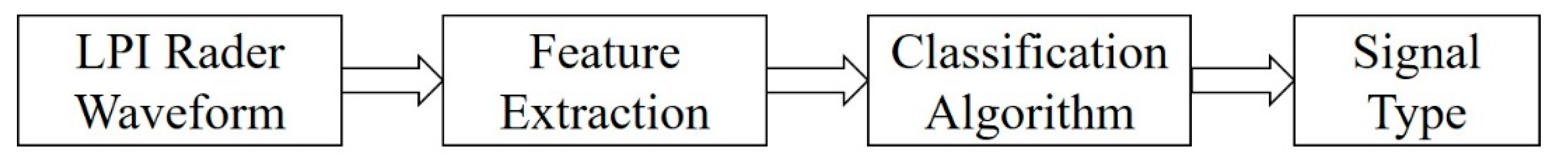
Recently, some scholars attempted to recognize radar signals in the time-frequency domain [12,13]. The general process of radar signal recognition includes time-frequency transformation, feature extraction, and classification, as shown in Figure 1. In [14], the Choi–Williams distribution (CWD) is used to process radar signals in the time and frequency domain simultaneously. Next, useful features extracted using image processing techniques are used to realize the recognition of five kinds of radar signals. Under the condition of SNR = 0 dB, the recognition accuracy reaches above 80%. Zhang et al. [15] propose to extract features of radar signals from both time and time-frequency domain, and achieve signal classification using the Elman neural network (ENN) based on the extracted features. This method achieves 94% recognition accuracy for eight kinds of signals when the signal-to-noise ratio is −2 dB, but shows a low recognition rate for Frank codes and P codes. The literature in [14] and the literature in [15] employ traditional machine learning methods to manually extract features from radar signals or signal time-frequency images. However, manual feature extraction is time-consuming and requires the assistance of expert knowledge.
In the past few years, deeper learning techniques have made great breakthroughs in various pattern recognition tasks, providing inspiration for radar signal recognition. Therefore, deeper learning has gradually become more widely used in radar signal recognition. Zhang et al. [16] presented two classifiers based on CNN and the Error-Encoding Network (ENN), respectively, to identify 12 radar signals. When the signal-to-noise ratio is −2 dB, the recognition accuracy is 94.5%, but the recognition rate of P code is low. In the literature [17], Wan et al. proposed an LPI radar waveform recognition system based on a convolutional neural network and a tree-based pipeline optimization tool (TPOT). The system performs convolution training on the CWD time-frequency images, and then realizes signal classification through the TPOP classifier. However, it has a low recognition rate for P3 and P4 codes. In the literature [18], Guo et al. proposed an automatic classification and recognition system based on CWD and deep convolutional neural network transfer learning. The CWD time-frequency image is sent to the pre-training model of the deep convolutional network for feature extraction. Finally, the extracted features are sent to SVM to realize signal recognition, but this algorithm has a low recognition rate for T1-T4 codes. When the signal-to-noise ratio is −6 dB, the recognition accuracy of eight kinds of signals is about 82%. Therefore, it is still a challenging problem to identify more types of LPI radar signals under a low signal-to-noise ratio.
To solve the problem of the difficulty of feature extraction under low SNR and the low recognition rate of various types of signals, in this paper, we propose a new approach for LPI radar signal recognition based on an asymmetric dual-channel CNN and feature fusion. Specifically, we first convert the 1D time-domain LPI radar signals into 2D time-frequency images using the CWD transformation, and design a dual-channel CNN model for feature extraction, which is different from the work in [16,17]. In the process of feature extraction, the high-level features extracted by CNN have rich semantic information, but some perceptual details may be lost. Therefore, we add a channel to extract the low-level features of the images through the HOG operator, which contains more location and detail information. Further, we use the MLP network to fuse these features from two channels. Finally, the fused features are fed into the Softmax classifier to realize the recognition of 12 LPI radar waveforms. Extensive experiments demonstrate the superiority and robustness of the proposed approach in radar signal recognition. In summary, the main contributions of the paper are listed below:
(1) We present a new approach for LPI radar signal recognition based on a dual-channel CNN model to improve the recognition accuracy under low SNR.
(2) A dual-channel CNN model is proposed to extract features of time-frequency images at different levels, which are further fused via an MLP network to the mutual benefit of both components.
(3) We give a comparison view to evaluate the proposed approach, and the experimental results show that the approach outperforms other state-of-the-art methods in recognition accuracy and stability.
The structure of this article is mainly composed of the following sections: In Section 2, we first introduce the overall framework of the proposed approach. Section 3 presents the preprocessing method for the LPI radar signals. The feature extraction process and the dual-channel CNN model are introduced in Section 4. In Section 5, we describe the details of feature fusion and signal recognition. Section 6 presents the experimental results and analysis. Finally, we conclude this work in Section 7.
2. Overview of the Proposed Approach
We first present the basic concepts used in this paper. We assume that the radar signal received by the electronic reconnaissance broadband receiver is generally composed of the signal and Gaussian white noise [19]. The signal model can be described as:
where and represent the signal and the noise, respectively. is the signal amplitude; is the phase function. We consider 12 types of LPI radar waveforms: frequency-shift keying (4FSK), linear frequency modulation (LFM), phase shift keying (BPSK), five polyphase codes (P1–P4, Frank), and four polytime codes (T1–T4). In order to achieve the recognition of these 12 radar signals under a low signal-to-noise ratio, we propose a new approach based on two-channel CNN feature fusion.
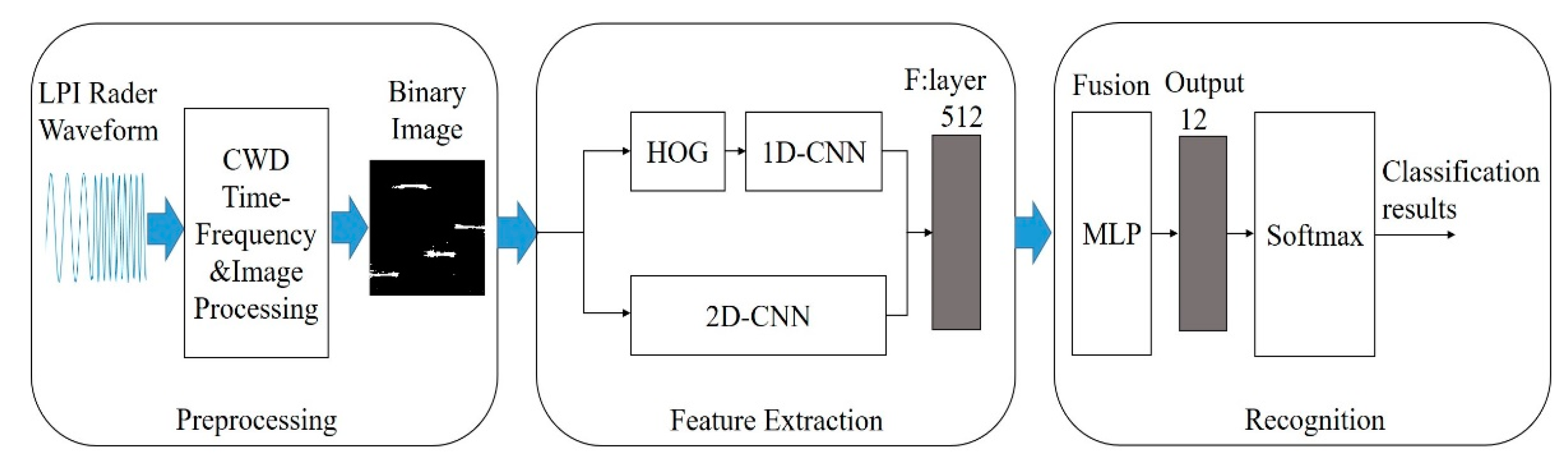
Figure 2 presents an overview of the proposed approach, which is mainly composed of three parts: preprocessing, feature extraction, and recognition. First, in the preprocessing part, we perform CWD transformation on the received LPI radar signal to obtain a two-dimensional time-frequency image. The time-frequency image is then processed by cropping, graying, bicubic interpolation, and binarization. In the feature extraction part, the pre-processed image is used for feature extraction through two channels, respectively. The first channel extracts the HOG features of the image and subsequently reduces the dimension of the HOG features based on one-dimensional CNN. The two-dimensional convolution channel directly extracts the convolutional features from the image. The features obtained from the two channels are fused through an MLP network. In the recognition part, the fused features are further dimensionally reduced and fed into the classifier to output the corresponding class labels. Finally, the model is saved for signal prediction after training. The details of each part of the framework will be described separately in the following sections.
3. Signal Preprocessing
The preprocessing of the LPI radar signal is the key step in the proposed framework; this step involves the CWD transformation of 1D signals to 2D time-frequency images, as well as some image processing operations. Moreover, due to the complex electromagnetic environment, there is significant noise in the received signal. Although the time-frequency processing of radar time-domain signals can effectively suppress noise interference, there may still be interference information in the time-frequency images. Therefore, some image processing operations, such as graying and binarization, are necessary to further eliminate interference before feature extraction. In this section, we mainly introduce the specific process involved in signal preprocessing.
3.1. CWD Transformation
The radar signal time-frequency analysis of CWD was proposed by H. Choi and J. Williams in 1989; it can effectively prevent the occurrence of cross-terms. Therefore, CWD is widely used in radar signal time-frequency analysis [20].
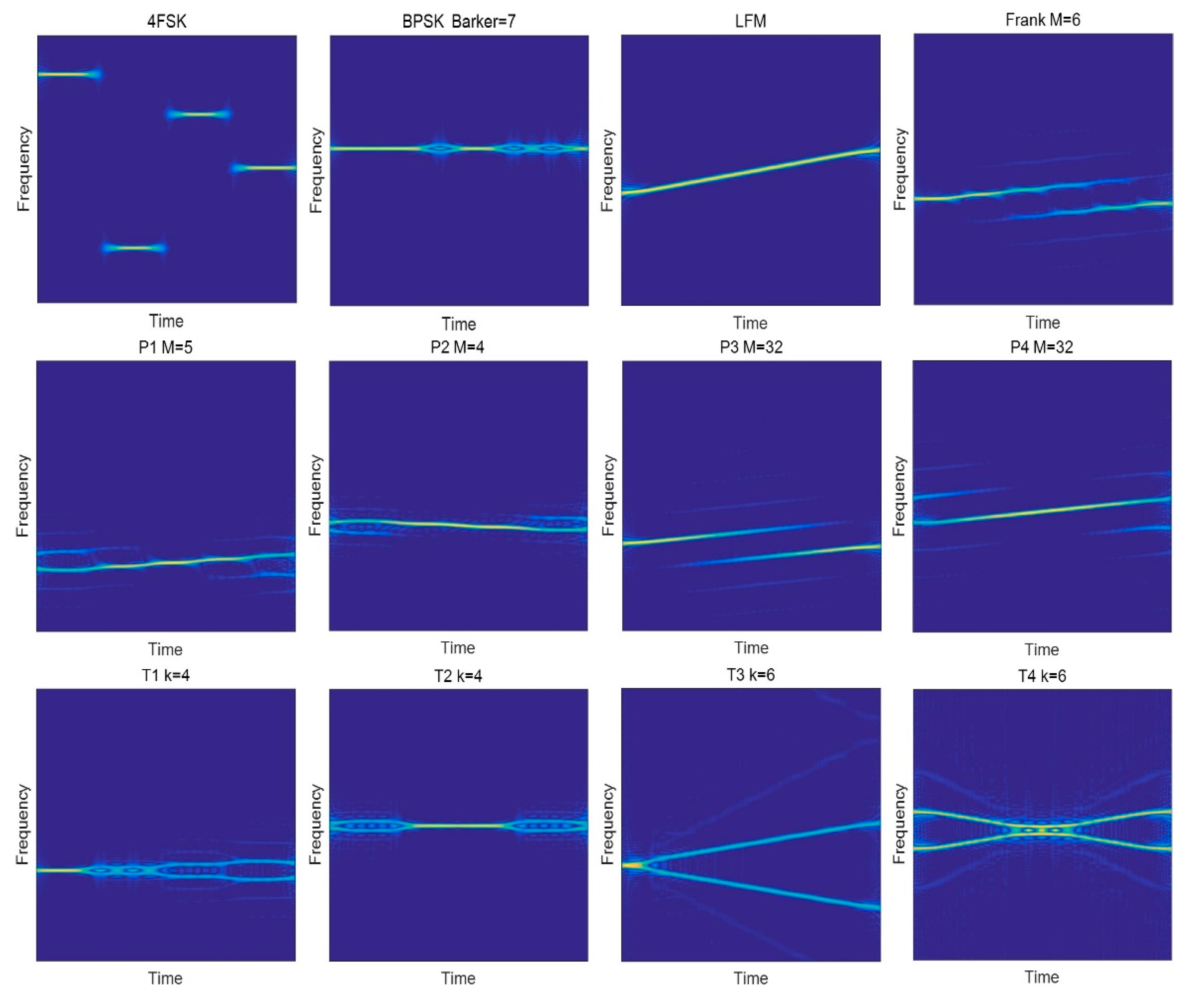
In the Equations (2) and (3), represents the output of CWD time-frequency analysis, represents time, represents frequency, represents kernel function, and represents attenuation factor. The parameter is a controllable factor which determines the bandwidth of the filter, and the cross-interference can be effectively suppressed by controlling the value. In this article, we chose to balance cross-interference and signal resolution. Figure 3 shows the results of the CWD transformation of the 12 types of LPI radar signals.
3.2. Time-Frequency Image Preprocessing
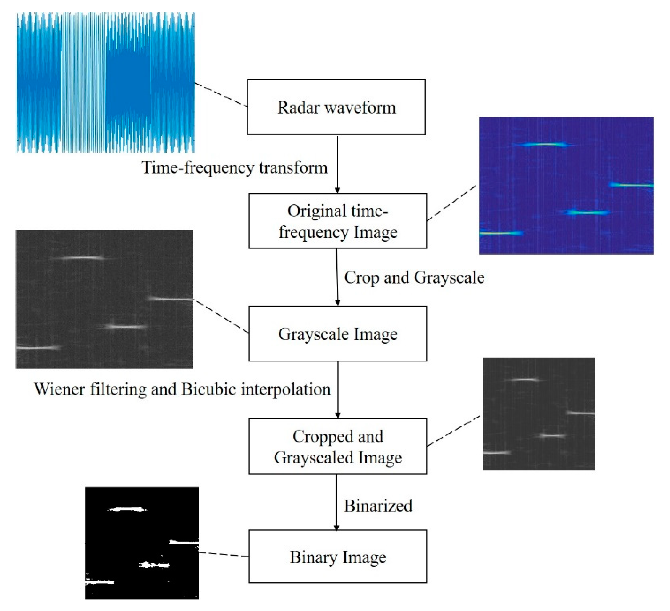
The specific procedure for radar signal preprocessing is shown in Figure 4. The received radar signal is first transformed into a time-frequency image; then, the original image with 656 × 875 pixels is cropped into an image with 535 × 679 pixels, from which a gray-scale image is derived by performing gray-scale processing. Subsequently, Wiener filtering is conducted on the grayscale image to reduce the noise interference in the image. Finally, bicubic interpolation and binarization are used to reduce both noise and the amount of image matrix data; thus, an image of 224 × 224 pixels is obtained.
4. Feature Extraction and Dual-Channel CNN Model Design
Feature extraction is the main element of the entire framework, which takes a time-frequency image input and produces a latent-feature representation for each image using a dual-channel CNN model. In this section, we mainly introduce the process of extracting the features (including HOG features and image features) and designing the dual-channel CNN model in detail.
4.1. Feature Extraction
In the feature extraction module, the features extracted from a time-frequency image include two parts, i.e., the HOG features and the image features, which are obtained using a dual-channel CNN model. The first channel based on the one-dimensional convolutional neural network is used to extract the HOG features by gradient calculation and histogram construction, and to perform dimensionality reduction. The specific process of HOG feature extraction will be described in detail in conjunction with the dual-channel CNN model in the following subsection. Moreover, to improve the signal recognition accuracy, we employ a two-dimensional convolutional neural network as the second channel to obtain discriminative features from time-frequency images. The features obtained through the dual-channel CNN model are fused by an MLP and get a low-dimensional feature representation. For the feature extraction module, the whole CNN model takes the time-frequency images of the LPI radar signals as input and is jointly trained with the downstream recognition task. In order to extract the optimal features, an adaptive learning rate method is used during the training. The initial learning rate is set to 0.002, and each iteration is adjusted to 0.9 times the original learning rate, which can effectively avoid the falling into a local optimum and prevent oscillations near the optimal solution due to too large a learning rate. The CNN model stops training when the generalization error is no longer decreasing, and the results are saved for prediction.
4.2. Dual-Channel Convolutional Neural Network Model
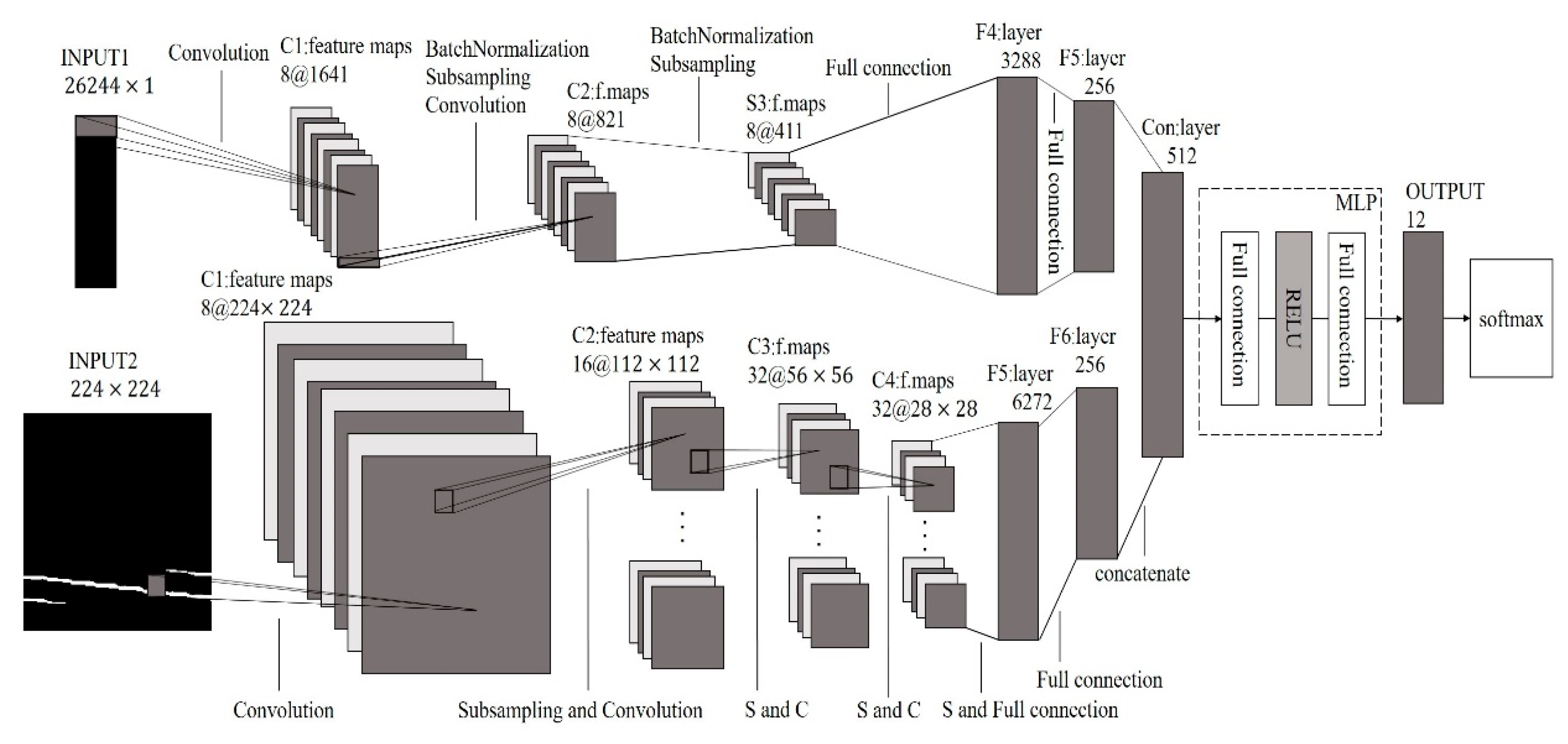
Inspired by the symmetry theory, we proposed an asymmetric dual-channel CNN model for feature extraction that sufficiently integrates the signal spectral features and signal contour features to improve the performance of radar signal recognition. The inputs of both channels of the model are the binarized time-frequency images. The one-dimensional CNN channel is used to extract the HOG features, and the two-dimensional convolution channel is used to extract the image features. Then, the features extracted from the two channels are fused. Finally, the fused features produced by the MLP network are used for the classification task. The architecture of the proposed dual-channel CNN model is shown in Figure 5.
4.2.1. One-Dimensional Convolution Channel
In image processing, the HOG feature parameters are generally used for object detection by calculating gradient information in images. The HOG operator divides an image into several cells and calculates the gradient of the pixel in each cell and the histogram of the direction of the object edge. It then counts the amplitudes of the histograms and combines them to form the HOG feature parameters. Because the gradient mainly exists in the edge area of the object, the algorithm can describe the signal edge, inflection point, and shape of the image through the calculated signal local area gradient and the direction edge density [21]. Based on this idea, the HOG feature extraction is introduced into the time-frequency image analysis to realize the detection of the edge, shape, and change characteristics of the time-frequency domain signal. Moreover, after the CWD time-frequency transformation and image binarization, the contour of the signal line is clearer and the inflection point is more obvious, enhancing the ability of the HOG operator to extract effective gradient values as feature parameters. The specific implementation process of the HOG feature extraction algorithm is as follows:
- Gradient calculation
Given an original image, it is convolved through the gradient operator to obtain the gradient component in the -axis direction (rightward is the positive direction); then, the gradient component in the -axis direction can be obtained by using the gradient operator . represents the value of pixel on the image; the specific calculation is shown in Equations (4) and (5):
The gradient amplitude and gradient direction at pixel can be expressed as Equations (6) and (7), respectively:
- 2.
- Gradient Direction Histogram Construction
The gradient direction is divided into nine angular regions at 180 degrees. These nine corner areas are used as the abscissa of the histogram. Then, the gradient value and gradient direction calculated for each pixel are mapped to nine corner regions. Finally, the nine amplitudes of the histogram are counted as the nine-dimensional feature vector of the corresponding cell [22]. Every 2 × 2 cell forms a block, and by moving the block on a 224 × 224 image, the feature number of a picture can be obtained as 4 × 9 × 27 × 27 = 26,224.
We design a one-dimensional convolutional network to reduce the dimension of the HOG features. Therefore, the 26,244-dimensional HOG features extracted above are fed into the one-dimensional convolution channel to obtain the low-dimensional vector representation. This channel mainly includes two modules. Each module contains a convolutional layer, a pooling layer, a batch normalization layer, and a dropout layer. The original HOG feature is extracted by two modules to obtain 8 × 821 data. In order to prevent the data from overfitting, we add a Dropout layer. At the same time, we have also added the batch standard layer, which will form a positive distribution through the data of Dropout, which is conducive to highlighting the features. The obtained feature matrix is then flattened and transformed into a one-dimensional feature vector that measures 256 × 1 through the fully connected layer.
4.2.2. Two-Dimensional Convolution Channel
The two-dimensional convolution channel is mainly used to extract discriminative features from time-frequency images, and it includes four convolutional layers and two fully connected layers. As is shown in Figure 4, the input image size is , which is fed into the convolutional layer with the convolution kernel size , and we achieve the C1 layer of size . Before the next convolution, the features in the C1 layer are selected by adding a sampling layer that can balance the relationship between the previous convolutional layer and the next convolutional layer while reducing the amount of calculation. Following the sampling layer and the convolutional layer, a C2 layer with a size of is obtained. After two more convolutions and samplings, we finally achieve a C4 layer of size and connect the feature map of the C4 layer to the two fully connected layers to obtain a contact feature with 256 dimensions.
5. Feature Fusion and Recognition via MLP
The recognition module is the last part of the proposed framework in this work; it directly infers the class label of the LPI radar signals based on the signal feature representation obtained in the previous stage. As mentioned above, the final feature representation of the radar signal consists of 1D CNN features and 2D CNN features. To obtain consistent feature representation, we fuse the features from the two sources using an MLP network with two hidden layers before recognition, instead of directly concatenating them. The number of the neurons for each hidden layer is determined from the output of the previous layer. Moreover, the feature fusion process further reduces the dimensionality of the features so that the subsequent classifier can effectively complete the classification task.
In the recognition module, we adopt the most-used Softmax classifier [23], which is an extension of the binary classification to multi-classification. Through Softmax calculation, the linearly weighted output value is converted into a probability distribution. The mathematical expression of the Softmax classification is shown as Equation (8), where is the number of final output categories (), is the output vector of the MLP for sample , and is the probability calculated by Softmax. From the formula, we can see that the Softmax function converts the output value of the multi-classification to a probability distribution that takes it to 1. As shown in Figure 4, the features (512 dimensions) from the two channels are purified and fused through the first hidden layer of the MLP to obtain a 256-dimensional feature. The resulting feature is connected to the second hidden layer to obtain a 12-dimensional vector, which represents 12 different LPI radar waveforms. Finally, the output vector is fed into the Softmax classifier for signal classification. At the same time, we optimize the model through the cross-entropy loss function, which is expressed as shown in Equation (9), where is the sign function, and reflects the actual deviation of the output from the expected output. In order to reduce the bias, we optimize the weights and biases by gradient descent, and then acquire the optimal model.
6. Experimental Results and Analysis
In this section, we verify the effectiveness of the proposed approach on the simulation platform with the specific parameters shown in Table 1. The section consists of four parts. The first part gives the simulation parameters of the low probability interception radar signals, the second part verifies the recognition accuracy of the model, the third part verifies the effectiveness of the model with comparative experiments, and the last part verifies the robustness of the approach.
6.1. Signal Generation
In this work, we select 12 typical radar signals including 4FSK, LFM, BPSK, FRANK, P1–P4, and T1–T4 for our experiments. Since different radar signals have different parameters, for the convenience of description, a uniform distribution based on the sampling frequency is used to uniformly represent the parameters; for example, represents a random number with a parameter range between .The initial frequency of the LFM signal is set between U(1/16) and U(1/8). The Barker code number of the BPSK signal is randomly selected from 7, 11, and 13, and the center frequency is set between U (1/8) and U (1/4). The four hopping frequencies of the 4FSK signal are between U(1/80) and U(1/2). For the T1-T4 signals, we set the number of basic waveform segments in the interval [4,5]. For the Frank signal, the phase control parameter M is 4–8. For the P1–P4 polyphase codes, the parameters are similar to Frank codes. The detailed parameters are shown in Table 2. In the experiment, the SNR range is −6~10 dB, and the step size is 2 dB. In each SNR, 600 samples are generated for each signal, of which 420 samples are used for training, and the remaining 180 samples are used for testing.
6.2. Recognition Accuracy Analysis
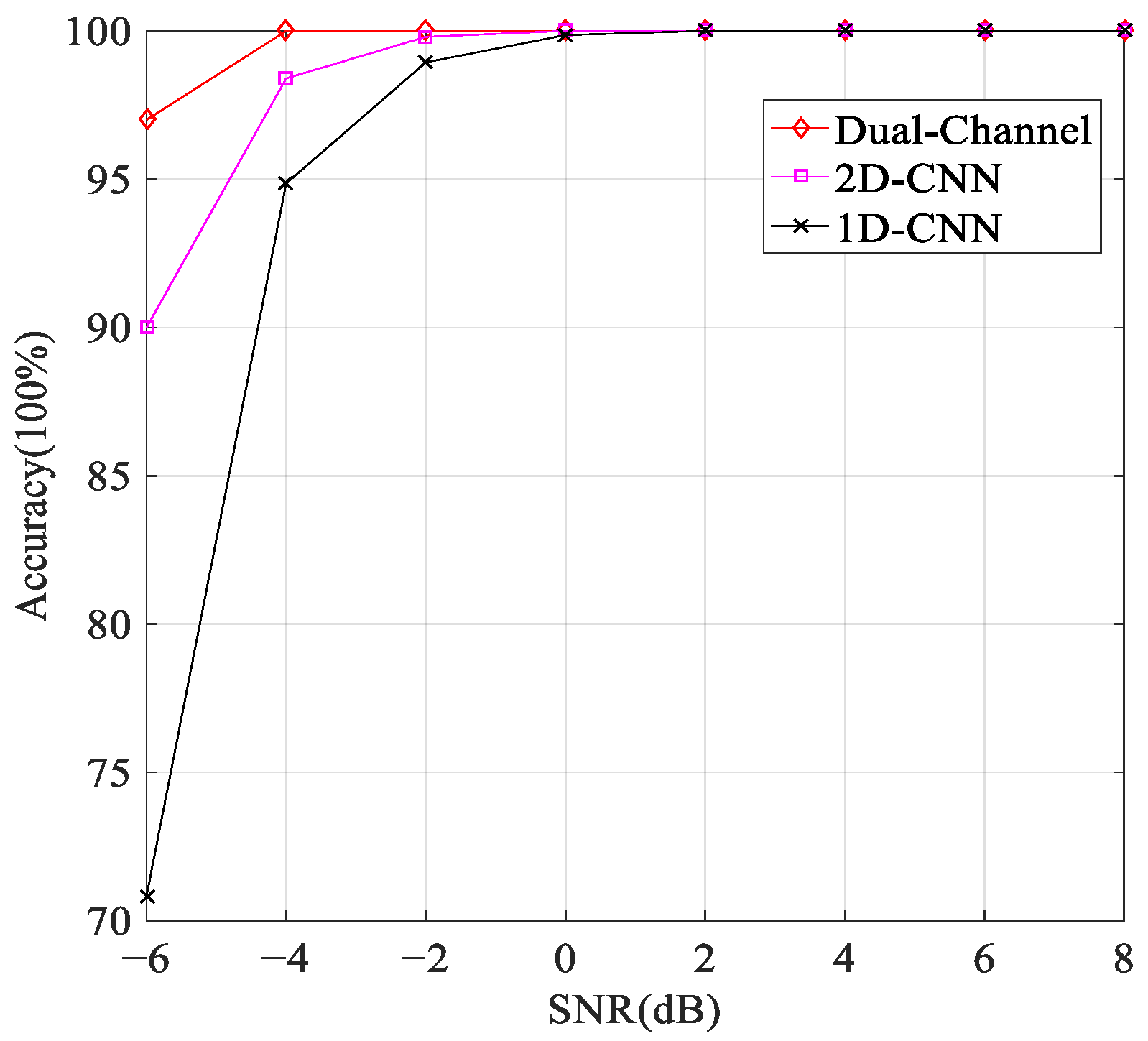
In order to prove the effectiveness of the dual-channel model, we compared the recognition accuracy of the dual-channel convolutional neural network to that of the respective single-channel convolutional neural networks. The simulation result is shown in Figure 6.
It can be seen from Figure 6 that the average recognition accuracy of the dual-channel model is higher than that of the single-channel model. Since it is difficult for a single feature to fully describe the features of radar signals, we propose a two-channel model that extracts convolutional features and HOG features simultaneously. The convolutional neural network can extract the rich hidden features of the signal time-frequency images, and the HOG feature can enhance the stability and robustness of the model; thus, the fusion of the two channel features can further improve the performance of the model. At the same time, in order to solve the problem of network overfitting and gradient disappearance, we add the Dropout layer and batch normalization layer to further improve the recognition rate for the radar signals. When the signal-to-noise ratio is −6 dB, the accuracy of dual-channel recognition is 7% higher than that of the 2D convolution channel and 26% higher than that of the 1D convolution channel. When the signal-to-noise ratio is −4 dB, the dual-channel recognition accuracy rate reaches 100%, which is 1.6% higher than that of the single-channel, which verifies the effectiveness of the dual-channel model.
6.3. Algorithmic Comparison Experiment
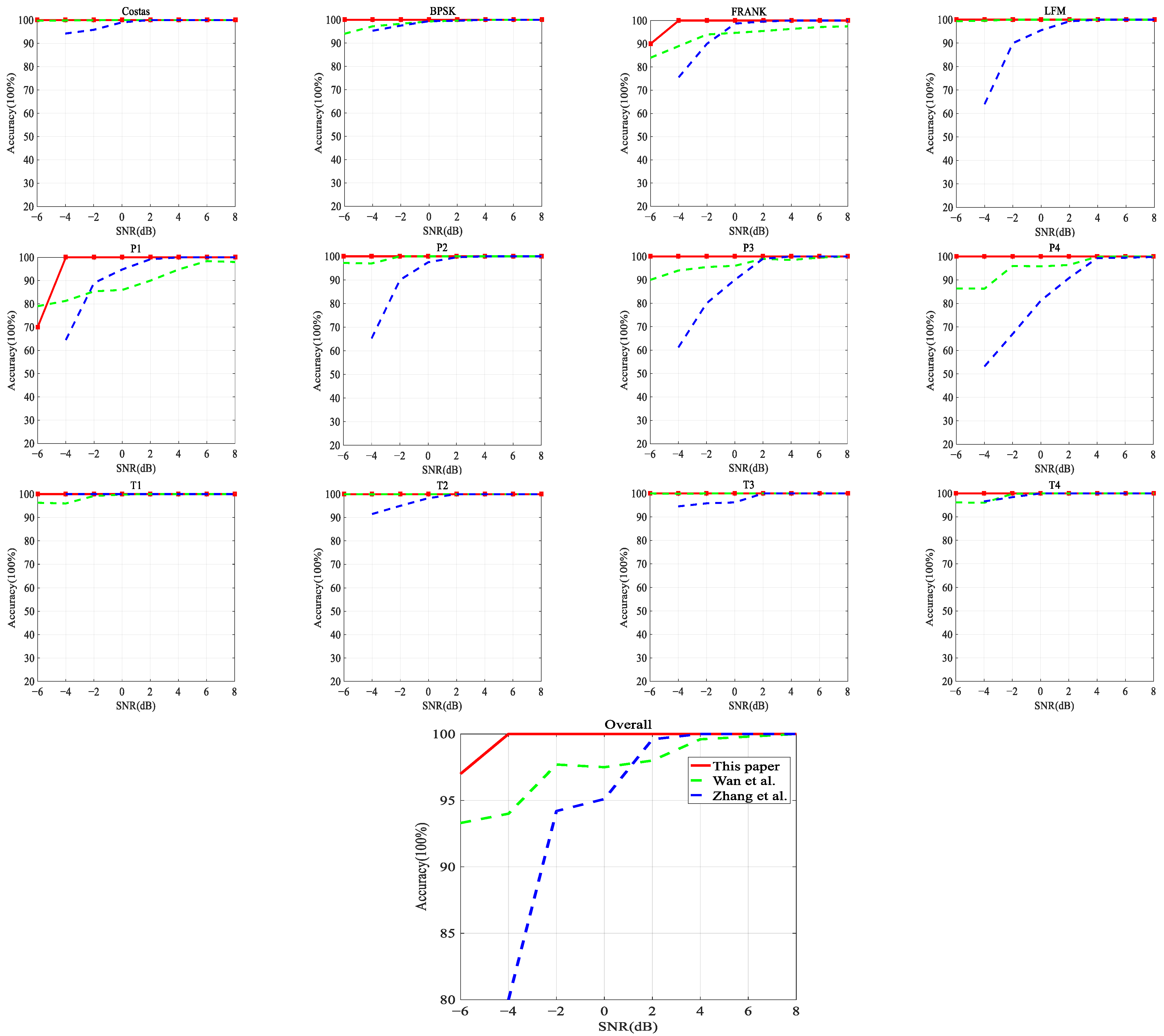
The following experiments mainly verify the relationship between the recognition accuracy and different signal-to-noise ratios. There are 480 groups of sample data used for training under each signal-to-noise ratio, and the remaining 120 groups are tested. At the same time, we also compare our method with the methods proposed by Wan et al. [17] and Zhang et al. [16]. The experimental results are shown in Figure 7.
As shown in Figure 7, the first 12 subfigures show the recognition accuracy of the algorithms for these 12 radar signals under varying SNR. Despite minor differences, these subfigures exhibit the same trend, i.e., the recognition rate of the algorithms subsequently increases significantly with the increasing SNR. When the signal-to-noise ratio is less than −2 dB, the recognition rate increases rapidly. When the signal-to-noise ratio is greater than −2 dB, the recognition rate increases slowly and eventually tends to be stable. Specifically, when the signal-to-noise ratio is greater than −6 dB, the recognition accuracy of our method on Costas, LFM, and T1–T4 signals is basically the same as that noted by Wan et al., which is close to 100%. The recognition rate of our method for BPSK signals is 100%, but the recognition rate of the method used by Wan et al. is about 94%. When the signal-to-noise ratio is −4 dB, the system’s recognition rate of P3 and P4 signals is 100%; the recognition accuracy of Wan et al.’s method is about 90%, and the recognition accuracy of Zhang et al.’s method is about 60%. Although the recognition accuracy of Frank and P1 signals at −6 dB is lower than that using Wan et al.’s method, as the signal-to-noise ratio increases to −4 dB, the recognition rate of this method reaches 100%, which is about 20% higher than Wan et al.’s method. Moreover, the last subfigure in Figure 7 demonstrates the overall recognition accuracy for the three approaches. At −4 dB, the recognition accuracy of this system is about 5% higher than that of Wan et al.’s method and about 20% higher than that of Zhang et al.’s method. With the increase of the signal-to-noise ratio, the accuracy of Wan et al.’s method increases slowly. It can be seen that the proposed approach has better performance under a low signal-to-noise ratio.
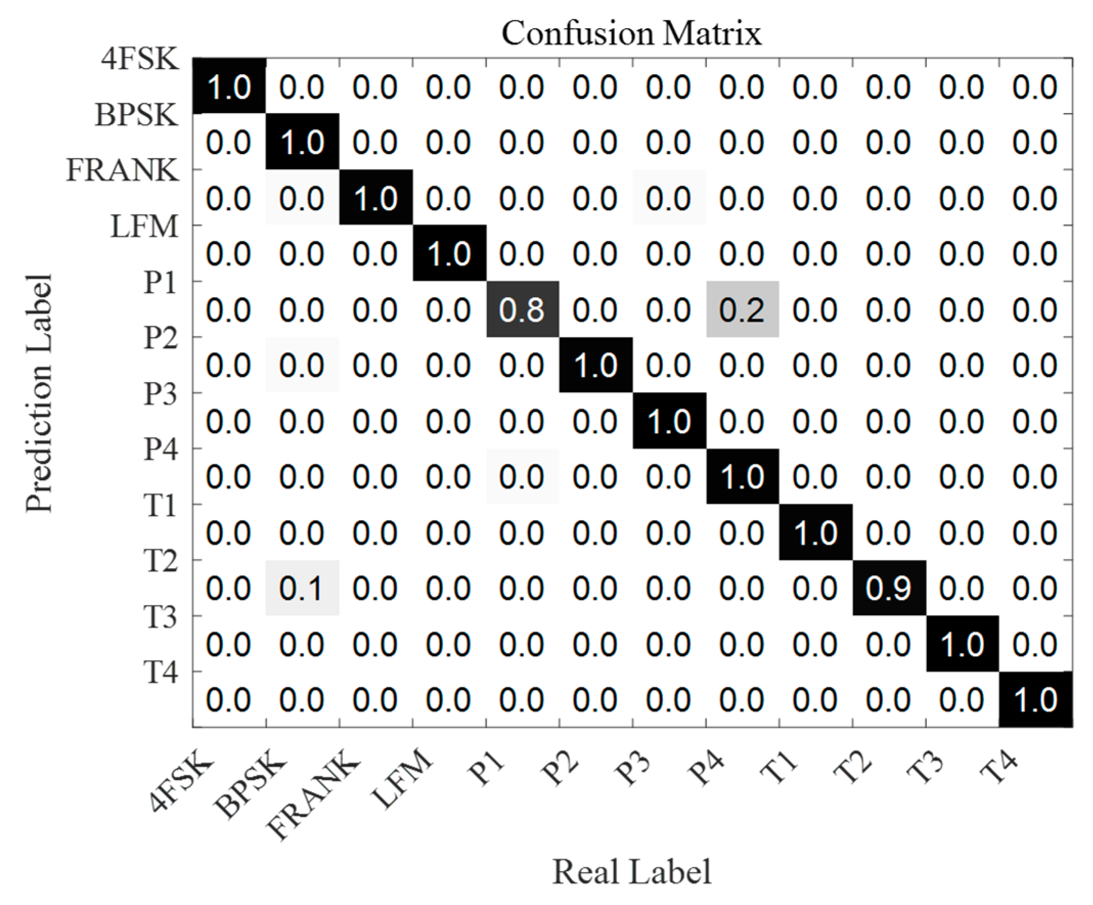
In addition, it can be seen from Figure 8 that some similar signal time-frequency images are easily confused under the interference of noise when the SNR is −6 dB. In our approach, the recognition accuracy for P1 codes is 80%, and 20% are misjudged as P4 codes. The recognition rate for T2 signals is 90%, and 10% are misjudged as BPSK signals.
6.4. Robustness Experiment
In order to verify the robustness of the algorithm, the radar signals are trained and tested under a mixed signal-to-noise ratio, and the robustness of the model is verified by testing the accuracy. The experimental results are shown in Table 3.
We save the model under a single signal-to-noise ratio, and then test the recognition accuracy of the model under different signal-to-noise ratios to test the robustness of the model. It can be seen from the experiments that the model still has a high recognition rate, and the accuracy rate is above 90%. Therefore, the model shows good robustness.
7. Conclusions
In this work, we propose a new method for LPI radar signal recognition based on dual-channel CNN and feature fusion to improve the recognition accuracy of LPI radar signals under the condition of low SNR. The proposed approach includes three modules: signal preprocessing, feature extraction, and feature fusion and recognition. The signal preprocessing module mainly converts 1D signals into 2D time-frequency images by CWD transformation for use in deep learning models. Next, we design a dual-channel CNN model to extract the HOG features and image features simultaneously from the time-frequency images. Compared with the baseline methods, the dual-channel model can simultaneously extract low-level features and high-level features of time-frequency images that mutually benefit from both components and can better characterize signal characteristics. The features from the two channels are fused via the MLP network to further improve the robustness and recognition accuracy of the model. Finally, the Softmax classifier is used to achieve the classification of the radar signals. The experimental results show that the method has a high recognition accuracy for typical radar signals under low SNR. It provides a feasible solution for radar signal recognition in complex electromagnetic environments.
In future work, we aim to conduct more in-depth research, particularly on dataset construction and feature fusion. At present, most of the training data and test data from related work are obtained based by simulation, the interference is relatively simple, and the recognition accuracy is better at low signal-to-noise ratio. However, in the real battlefield environment, in addition to white noise, there are interferences, such as traffic signals, and the recognition accuracy will be greatly reduced. Therefore, our next study will try to generate training data and test data using a hardware-in-the-loop simulation system, in which real-world scenarios are approximated by transmitters and receivers, and the received signal is trained and recognized. This type of research will make our work more valuable. In feature fusion, we will study the methods of measuring and combining different features [25], as well as dealing with the redundancy and differences between features.
Author Contributions
Conceptualization, D.Q. and X.W.; methodology, Z.T.; software, Z.T. and W.Z.; validation, Z.T. and C.Q.; formal analysis, D.Q.; investigation, Z.T. and C.Q.; writing—original draft preparation, Z.T.; writing—review and editing, X.W. and W.Z; visualization, Z.T.; supervision, D.Q and X.W.; funding acquisition, D.Q. and X.W. All authors have read and agreed to the published version of the manuscript.
Funding
This work was supported in part by The Natural Science Foundation of Zhejiang Province (No.LQ20F020021), in part by the Open Project of Zhejiang Key Laboratory of Electromagnetic Wave Information Technology and Metrology Testing (No.2019KF0003).
Institutional Review Board Statement
Not applicable.
Informed Consent Statement
Not applicable.
Data Availability Statement
Not applicable.
Conflicts of Interest
The authors declare no conflict of interest.
References
- Tao, W.A.N.; Kaili, J.; Jingyi, L.; Yanli, T.A.N.G.; Bin, T.A.N.G. Detection and recognition of LPI radar signals using visibility graphs. J. Syst. Eng. Electron. 2020, 31, 1186–1192. [Google Scholar] [CrossRef]
- Shi, C.; Qiu, W.; Wang, F.; Salous, S.; Zhou, J. Cooperative LPI Performance Optimization for Multistatic Radar System: A Stackelberg Game. In Proceedings of the International Applied Computational Electromagnetics Society Symposium—China (ACES), Nanjing, China, 8–11 August 2019; pp. 1–2. [Google Scholar]
- Nandi, A.K.; Azzouz, E.E. Automatic analogue modulation recognition. Signal Processing 1995, 46, 211–222. [Google Scholar] [CrossRef]
- Dudczyk, J.; Kawalec, A. Specific emitter identification based on graphical representation of the distribution of radar signal parameters. Bull. Pol. Acad. Sci. Tech. Sci. 2015, 63, 391–396. [Google Scholar] [CrossRef]
- Gupta, D.; Raj, A.A.B.; Kulkarni, A. Multi-Bit Digital Receiver Design for Radar Signature Estimation. In Proceedings of the 3rd IEEE International Conference on Recent Trends in Electronics, Information & Communication Technology (RTEICT), Bangalore, India, 18–19 May 2018; pp. 1072–1075. [Google Scholar]
- Huang, G.; Ning, F.; Liyan, Q. Sparsity-based radar signal sorting method in electronic support measures system. In Proceedings of the 12th IEEE International Conference on Electronic Measurement & Instruments (ICEMI), Qingdao, China, 16–18 July 2015; pp. 1298–1302. [Google Scholar]
- Kishore, T.R.; Rao, K.D. Automatic intrapulse modulation classification of advanced LPI radar waveforms. IEEE Trans. Aerosp. Electron. Syst. 2017, 53, 901–914. [Google Scholar] [CrossRef]
- Iglesias, V.; Grajal, J.; Royer, P.; Sanchez, M.A.; Lopez-Vallejo, M.; Yeste-Ojeda, O.A. Real-time low-complexity automatic modulation classifier for pulsed radar signals. IEEE Trans. Aerosp. Electron. Syst. 2015, 51, 108–126. [Google Scholar] [CrossRef]
- Schleher, D.C. LPI radar: Fact or fiction. IEEE Aerosp. Electron. Syst. Mag. 2006, 21, 3–6. [Google Scholar] [CrossRef]
- Mingqiu, R.; Jinyan, C.; Yuanqing, Z.; Jun, H. Radar signal feature extraction based on wavelet ridge and high order spectral analysis. In Proceedings of the IET International Radar Conference 2009, Guilin, China, 20–22 April 2009; pp. 1–5. [Google Scholar]
- Wang, C.; Gao, H.; Zhang, X. Radar signal classification based on auto-correlation function and directed graphical model. In Proceedings of the IEEE International Conference on Signal Processing, Communications and Computing (ICSPCC), Hong Kong, 5–8 August 2016; pp. 1–4. [Google Scholar]
- Cohen, L. Time-frequency distributions-a review. Proc. IEEE 1989, 77, 941–981. [Google Scholar] [CrossRef] [Green Version]
- López-Risueño, G.; Grajal, J.; Sanz-Osorio, A. Digital channelized receiver based on time-frequency analysis for signal interception. IEEE Trans. Aerosp. Electron. Syst. 2005, 41, 879–898. [Google Scholar] [CrossRef]
- Zilberman, E.R.; Pace, P.E. Autonomous time-frequency morphological feature extraction algorithm for LPI radar modulation classification. In Proceedings of the International Conference on Image Processing, Atlanta, GA, USA, 8–11 October 2006; pp. 2321–2324. [Google Scholar]
- Zhang, M.; Liu, L.; Diao, M. LPI radar waveform recognition based on time-frequency distribution. Sensors 2016, 16, 1682. [Google Scholar] [CrossRef] [PubMed]
- Zhang, M.; Diao, M.; Gao, L.; Liu, L. Neural networks for radar waveform recognition. Symmetry 2017, 9, 75. [Google Scholar] [CrossRef] [Green Version]
- Wan, J.; Yu, X.; Guo, Q. LPI radar waveform recognition based on CNN and TPOT. Symmetry 2019, 11, 725. [Google Scholar] [CrossRef] [Green Version]
- Guo, Q.; Yu, X.; Ruan, G. LPI radar waveform recognition based on deep convolutional neural network transfer learning. Symmetry 2019, 11, 540. [Google Scholar] [CrossRef] [Green Version]
- Qu, Z.; Mao, X.; Deng, Z. Radar signal intra-pulse modulation recognition based on convolutional neural network. IEEE Access 2018, 6, 43874–43884. [Google Scholar] [CrossRef]
- Wang, H.; Diao, M.; Gao, L. Low probability of intercept radar waveform recognition based on dictionary leaming. In Proceedings of the 10th International Conference on Wireless Communications and Signal Processing (WCSP), Hangzhou, China, 18–20 October 2018; pp. 1–6. [Google Scholar]
- Zhang, S.; Wang, X. Human detection and object tracking based on Histograms of Oriented Gradients. In Proceedings of the Ninth International Conference on Natural Computation (ICNC), Shenyang, China, 23–25 July 2013; pp. 1–6. [Google Scholar]
- Korkmaz, S.A.; Akçiçek, A.; Bínol, H.; Korkmaz, M.F. Recognition of the stomach cancer images with probabilistic HOG feature vector histograms by using HOG features. In Proceedings of the IEEE 15th International Symposium on Intelligent Systems and Informatics (SISY), Subotica, Serbia, 14–16 September 2017; pp. 339–342. [Google Scholar]
- Rao, Q.; Yu, B.; He, K.; Feng, B. Regularization and Iterative Initialization of softmax for Fast Training of Convolutional Neural Networks. In Proceedings of the International Joint Conference on Neural Networks (IJCNN), Budapest, Hungary, 14–19 July 2019; pp. 1–8. [Google Scholar]
- Huynh-The, T.; Doan, V.S.; Hua, C.H.; Pham, Q.V.; Nguyen, T.V.; Kim, D.S. Accurate LPI Radar Waveform Recognition with CWD-TFA for Deep Convolutional Network. IEEE Wirel. Commun. Lett. 2021, 10, 1638–1642. [Google Scholar] [CrossRef]
- Ben Atitallah, S.; Driss, M.; Boulila, W.; Koubaa, A.; Ben Ghézala, H. Fusion of convolutional neural networks based on Dempster—Shafer theory for automatic pneumonia detection from chest X-ray images. Int. J. Imaging Syst. Technol. 2022, 32, 658–672. [Google Scholar] [CrossRef]
Figure 1.
A flowchart of LPI radar signal recognition.

Figure 2.
The framework of the proposed approach for LPI radar signal recognition.

Figure 3.
The CWD transformation images of 12 kinds of LPI radar signals.

Figure 4.
The time-frequency image preprocessing flowing chart. In the chart, we take the 4FSK signal with SNR = 0 dB as an example to illustrate this process.
Figure 4.
The time-frequency image preprocessing flowing chart. In the chart, we take the 4FSK signal with SNR = 0 dB as an example to illustrate this process.

Figure 5.
The architecture of the dual-channel CNN model.

Figure 6.
The comparison of the recognition accuracy on different CNN channels.

Figure 7.
The comparative experiment under different signal-to-noise ratios for each signal.

Figure 8.
The confusion matrix of 12 kinds of signals under −6 dB SNR.


Table 1.
The experimental environment.
| Item | Model/Version |
|---|---|
| CPU | Intel(R) Core(TM) i7-10875H |
| GPU | NVIDIA GeForce RTX 2060 |
| RAM | 16 GB |
| SOFTWARE | R2016b/Python 3.7 |
Table 2.
The simulation parameter list [24].
Table 2.
The simulation parameter list [24].
| Radar Waveform | Simulation Parameter | Ranges |
|---|---|---|
| Sampling frequency | 1 ( = 200 MHz) | |
| LFM | Initial frequency Bandwidth | |
| BPSK | Barker codes Carrier frequency | |
| 4FSK | Fundamental frequency | |
| Frank and P1 | Carrier frequency Samples of frequency stem M | |
| P2 | Carrier frequency Samples of frequency stem M | |
| P3 and P4 | Carrier frequency | |
| T1-T4 | Number of segments k |
Table 3.
The simulation parameter list.
| Saved Model/dB | Test Data/dB | Recognition Accuracy |
|---|---|---|
| −6 | 0 | 95% |
| −4 | 2 | 92.6% |
| −2 | 2 | 93% |
| 2 | −2 | 96.62% |
Publisher’s Note: MDPI stays neutral with regard to jurisdictional claims in published maps and institutional affiliations. |
© 2022 by the authors. Licensee MDPI, Basel, Switzerland. This article is an open access article distributed under the terms and conditions of the Creative Commons Attribution (CC BY) license (https://creativecommons.org/licenses/by/4.0/).
Share and Cite
MDPI and ACS Style
Quan, D.; Tang, Z.; Wang, X.; Zhai, W.; Qu, C. LPI Radar Signal Recognition Based on Dual-Channel CNN and Feature Fusion. Symmetry 2022, 14, 570. https://doi.org/10.3390/sym14030570
AMA Style
Quan D, Tang Z, Wang X, Zhai W, Qu C. LPI Radar Signal Recognition Based on Dual-Channel CNN and Feature Fusion. Symmetry. 2022; 14(3):570. https://doi.org/10.3390/sym14030570
Chicago/Turabian StyleQuan, Daying, Zeyu Tang, Xiaofeng Wang, Wenchao Zhai, and Chongxiao Qu. 2022. "LPI Radar Signal Recognition Based on Dual-Channel CNN and Feature Fusion" Symmetry 14, no. 3: 570. https://doi.org/10.3390/sym14030570
Note that from the first issue of 2016, this journal uses article numbers instead of page numbers. See further details here.