Variational Quantum Circuits to Prepare Low Energy Symmetry States

Abstract

We explore how to build quantum circuits that compute the lowest energy state corresponding to a given Hamiltonian within a symmetry subspace by explicitly encoding it into the circuit. We create an explicit unitary and a variationally trained unitary that maps any vector output by ansatz $A(\overrightarrow{\alpha })$ from a defined subspace to a vector in the symmetry space. The parameters are trained varitionally to minimize the energy, thus keeping the output within the labelled symmetry value. The method was tested for a spin XXZ Hamiltonian using rotation and reflection symmetry and $H_2$ Hamiltonian within $S_z=0$ subspace using $S^2$ symmetry. We have found the variationally trained unitary gives good results with very low depth circuits and can thus be used to prepare symmetry states within near term quantum computers.

1. Introduction

One of the most important problems quantum computers have been envisioned to solve is the simulation of Hamiltonian dynamics and computation of ground state energies. Phase estimation algorithm [1,2], despite solving this problem, requires circuits that run deep, something that cannot be afforded within the NISQ [3] era. Alternative algorithms based on hybrid models that make use of variational methods, for instance variational quantum eigensolvers (VQE) [4] and quantum imaginary time evolution [5], have been found to be more resilient to noisy quantum devices [6]. The strength of a variational method depends a lot on the variational ansatz that has been used for the simulation of the given state. Unitary coupled clusters [7] decomposed using trotterization [8], RBM ansatz [9] based models and using hardware efficient gates to create generalized layered models [10] are some of the circuit designs that have been studied under variational methods.

Solving for the low energy states that lie within a Symmetry subspace, i.e., labelled by a specified symmetry value, forms a sub class within the generalized constrained optimization problems, where the idea is to minimize a cost function subject to a given set of constraints. In cases where the operators of the cost function commute with that of the constraints, one could easily penalize the cost function with an additional term that captures the error in symmetry value [11]. Alternatively, one could design circuits that variationally only explore the symmetry subspace by defining the circuit using well defined structured features. These methods explore a smaller Hilbert space for optimization and are likely to converge faster. Barkoutsos et al. [12] used a particle conserving gate alongside a particle hole conserving representation to produce ground states of simple molecular systems. Gard et al. introduced a systematic way of preserving symmetry subspaces for particle number, total spin, spin projection, and time reversal [13].

Unlike previous studies, which aimed to provide algorithms for very specific symmetries, we would like to demonstrate the efficacy of two new techniques that can tackle any symmetry generically. We further compute the ground state energy of a given Hamiltonian constrained to lie within the specified symmetry subspace, i.e., the state is a eigenvector of the chosen symmetry operator with a user-defined eigenvalue.

The organization of the paper is as follows. In Section 2 we illustrate in detail the underlying theoretical framework of both the methods. In Section 3 we discuss the results using Heisenberg XXZ-Spin Hamiltonian and choose two symmetry operators pertinent to the system. We also explore a real molecular system ($H_2$) to filter singlet states of total spin angular momentum squared ($S^2$) as the corresponding symmetry operator. We conclude thereafter in Section 4 with a brief discussion of possible future extensions.

2. Method

Hybrid variational quantum algorithms have been extensively studied in the context of solving unconstrained [14,15,16,17] and even constrained optimization problems [11,18,19]. The primary workhorse of such methods revolve around iteratively minimizing a cost function through a usual gradient-based optimization scheme to tweak the parameters of the quantum circuit subsequently. The gradients of the cost–function are typically computed directly from the quantum circuit [20], for instance using a parameter shift method [21], while the succeeding parameter updates proceeds classically. Updates are expressed as expectation values of output states against some Hermitian operator that can be re-expressed as a Pauli string sum and computed independently using measurements on a basis that diagonalizes the operator or uses the Hadamard test [22]. The output state is typically representative of an ansatz that is expressive enough to explore a sizeable portion of the whole Hilbert space of dimension that scales as $2^n$ where n is the number of qubits used in the variational method. The chosen ansatz is generic and oblivious to the symmetry eigensector being sought.

In this work, we explore an alternative route. The cornerstone of our technique lies in its ability to confine the state-ansatz a priori to a particular eigenspace of the chosen symmetry operator even before the optimization for minimal energy is attempted. This is attained by building a variational state into the ansatz that selectively explores the symmetry-subspace of interest.

We now define the problem formally, which shall be attempted to be solved in this work. Let us consider a system characterized by a Hamiltonian H and let the complete set of symmetry operators for this system be a set $P={\left\{O_k\right\}}_{k=1}^N$ wherein $[H,O_m]=0\forall O_m\in P$. Thus, the set $H\bigcup P$ completely characterizes the state-space of the physical system. Given a symmetry operator $O_k\in P$, we would like to find to find the lowest energy state $|{\psi }^{*}\rangle$ within a sector labelled by specific symmetry value. This can be computed through solving the following optimization problem,

$$\begin{array}{ccc}\hfill |{\psi }^{*}\rangle & =& \underset{\psi (\overrightarrow{\theta })\in \Omega }{argmi{n}_{\psi (\overrightarrow{\theta })}}\langle \psi (\overrightarrow{\theta })\left|H\right|\psi (\overrightarrow{\theta })\rangle \hfill \\ \hfill such that \Omega & =& \left\{\right|x\rangle |O_k|x\rangle =S|x\rangle ,\forall |x\rangle \in {\mathbb{C}}^{2^n}\}\hfill \end{array}$$

(1)

where S is the user-specified eigenvalue of $O_k$ which labels the desired eigenspace and $\overrightarrow{\theta }$ are the variational parameters. Without loss of generality, one can envision that $|\Omega |=r$, i.e., the symmetry subspace, is r-dimensional.

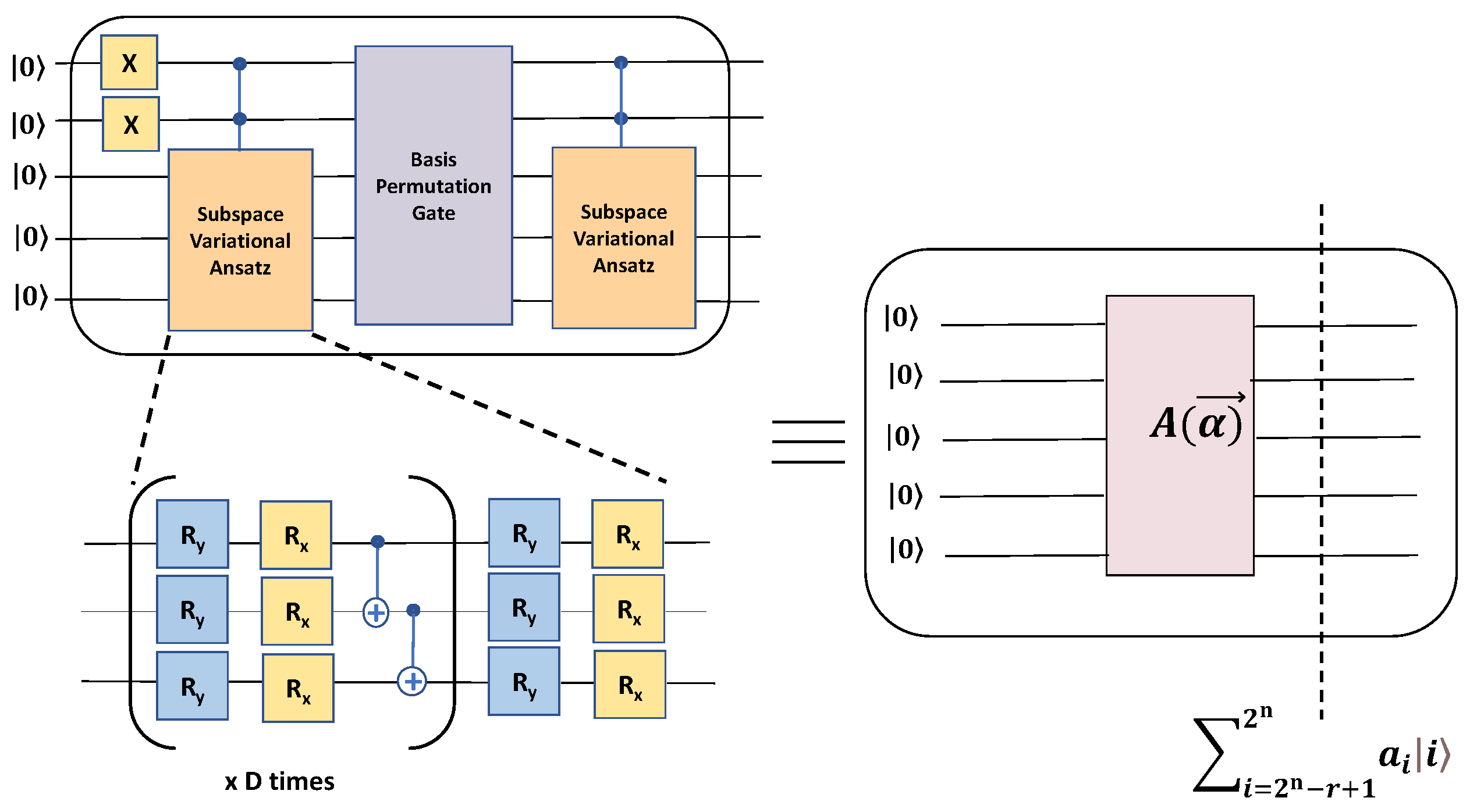
We start by first constructing a generic r-dimensional variational ansatz $A(\overrightarrow{\alpha }){|0\rangle }^{⨂n}$ which allows us to subsequently confine the acceptable state within the symmetry subspace $\Omega$ defined in Equation (1), where $A(\overrightarrow{\alpha })$ is the unitary creating the variational ansatz with $\overrightarrow{\alpha }$ being the corresponding parameters. If r is expressible as an exponentiation of 2, one could condition the variational circuit over the first $n-m$ qubits, where $m=lo{g}_2(r)$. Otherwise, we choose $m=\lfloor lo{g}_2(r)\rfloor$ and then use a permutation gate to swap in the basis states to match the size of the symmetry sector before applying another layer of variational ansatz. This ensures that $A(\overrightarrow{\alpha })$ creates an output state whose dimension matches the symmetry sector of interest. A discussion of the construction of Permutation gate to construct $A(\overrightarrow{\alpha })$ has been deferred to Appendix A. Mathematically, the action of the unitary $A(\overrightarrow{\alpha })$ can be envisioned as,

$$A(\overrightarrow{\alpha }){|0\rangle }^{⨂n}=\sum _{i=1}^{2^n}{a}_i(\overrightarrow{\alpha })|i\rangle =\sum _{i=2^n-r+1}^{2^n}{a}_i(\overrightarrow{\alpha })|i\rangle$$

(2)

wherein $|i\rangle$ denotes the computational basis states and $a_i(\overrightarrow{\alpha })$ are the respective coefficients parameterized over $\overrightarrow{\alpha }$. The last equality in Equation (2) follows from the fact that $a_i(\overrightarrow{\alpha })=0\forall i\le 2^n-r$. This allows us to create a variational ansatz over a r-dimensional subspace of ${\mathbb{C}}^{2^n}$, as is required. Figure 1 provides a schematic view of the circuit involved in the construction of ansatz $A(\overrightarrow{\alpha })$. We now present two different methods that differ in the post-processing of the ansatz $A(\overrightarrow{\alpha }){|0\rangle }^{⨂n}$ once created. As mentioned before, the ultimate goal of both the methods will be to map the computational basis states ${\left\{\right|i\rangle \}}_{i=2^n-r+1}^{2^n}$ onto the symmetry sub-space $\Omega$ using a unitary transformation and then obtain the minimal energy eigenstate in that subspace.

2.1. Method 1—Exact Unitary

This method uses an exact unitary that is composed of the eigenvectors of the symmetry operator. Let U be the unitary operator that diagonalizes $O_k$ i.e. $U={\sum }_{i=1}^{2^n}|{\varphi }_i\rangle \langle i|$ wherein $|{\varphi }_i\rangle$ are the eigenvectors of the symmetry operator $O_k$. Using the unitary U on the r-dimensional ansatz defined in Equation (2), we thus get,

$$UA(\overrightarrow{\alpha }){|0\rangle }^{⨂n}=\sum _{j=1}^{2^n}|{\varphi }_j\rangle \langle j|(\sum _{i=2^n-r+1}^{2^n}{a}_i(\overrightarrow{\alpha })|i\rangle )=\sum _{i=2^n-r+1}^{2^n}{a}_i(\overrightarrow{\alpha })|{\varphi }_i\rangle$$

(3)

where in the last equality of Equation (3) only the eigenvectors $|{\varphi }_i\rangle$${}_{i=2^n-r}^{2^n}$$\in \Omega$ survive. Operationally, the matrix U is constructed by stacking the r eigenvectors corresponding to eigenvalue S in the last r-columns. Note that the coefficients $a_i$ in Equation (3) are explicitly dependant on tunable parameters $\overrightarrow{\alpha }$ imparted from the ansatz $A(\overrightarrow{\alpha })$. We thereafter train these parameters $\overrightarrow{\alpha }$ by minimizing the energy of the output state using the Hamiltonian H of the system as follows,

$${\overrightarrow{\alpha }}^{*}=argmi{n}_{\overrightarrow{\alpha }} {}^{n⨂}\langle 0|A^{†}(\overrightarrow{\alpha })U^{†}HUA(\overrightarrow{\alpha }){|0\rangle }^{⨂n}.$$

(4)

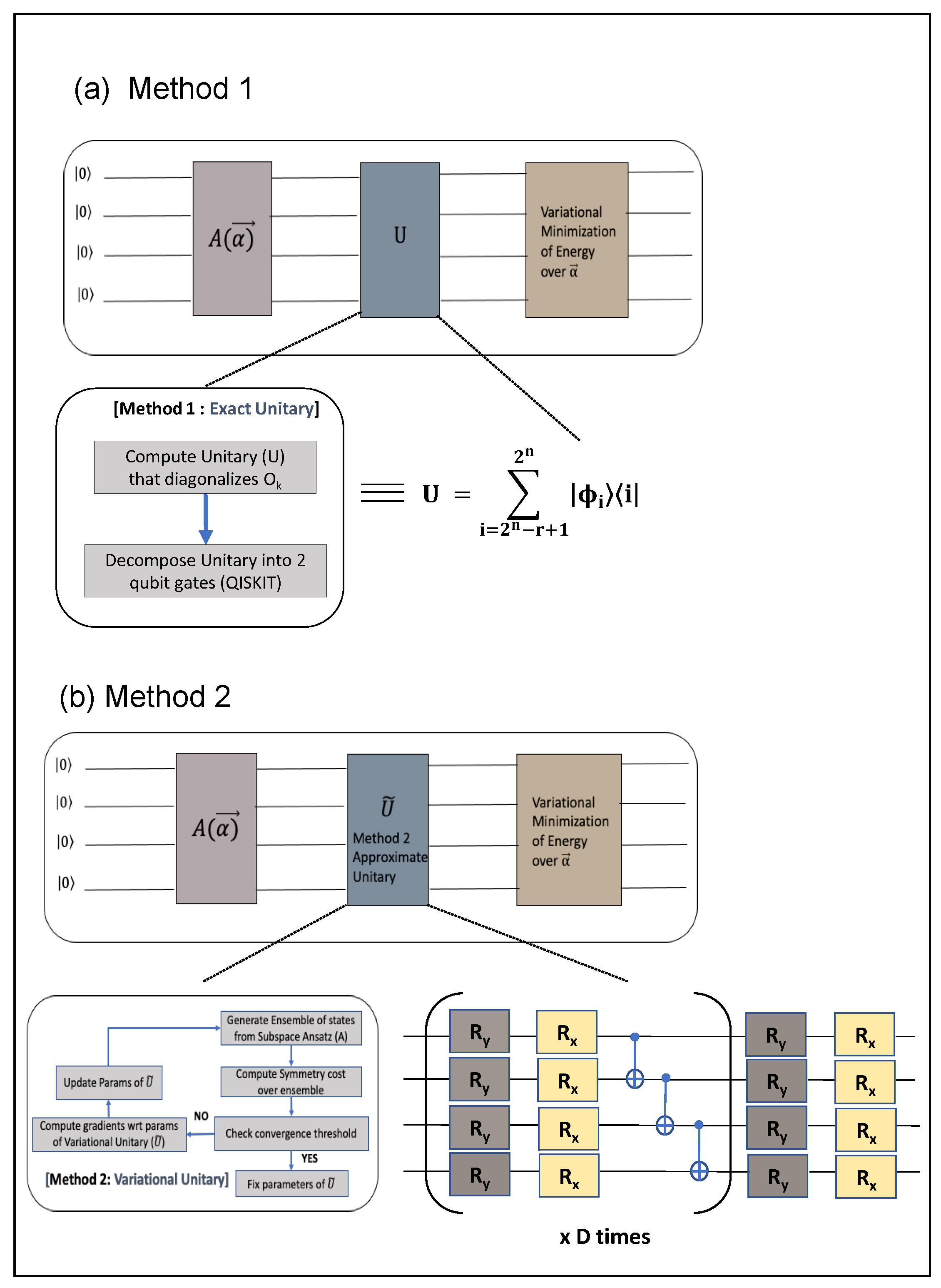
The minimization scheme in Equation (4) leads us to the minimal energy state within the symmetry subspace, as is required. As this method uses the exact unitary U, it shall work irrespective of any initial ansatz with an output that is restricted to the subspace. We schematically describe Method 1 in Figure 2a. This method, however, requires decomposing the matrix U into a sequence of elementary gates which, depending on the symmetry, may result in a quantum circuit with very large depth. To circumvent this drawback, we propose an alternative approach (Method 2), described next.

2.2. Method 2—Approximate Unitary Construction

In this method, instead of using the exact unitary U obtained from the diagonalization of the symmetry operator $O_k$ as introduced in Method 1, we approximate it using a parameterized ansatz $\tilde{U}$ which allows for a low depth quantum circuit construction. Operationally, we use the same ansatz as in $A(\overrightarrow{\alpha })$ for constructing $\tilde{U}(\overrightarrow{\theta })$ and then learn the parameters variationally by minimizing the cost function $\langle {(O_k-S\mathsf{𝟙})}^2\rangle$, where S is the desired eigenvalue. The state on which the unitary $\tilde{U}(\overrightarrow{\theta })$ acts is $A(\overrightarrow{\alpha }){|0\rangle }^{⨂n}$, as introduced in the previous section. The variational minimization over $\overrightarrow{\theta }$ is done over many realizations of the parameter set $\overrightarrow{\alpha }$, which is akin to an averaging procedure over the underlying sampling distribution $p(\overrightarrow{\alpha })$. Mathematically, the parameter set $\overrightarrow{\theta }$ is learned as follows,

$${\overrightarrow{\theta }}^{*}=argmi{n}_{\overrightarrow{\theta }} {{\langle }^{n⨂}\langle 0|A^{†}(\overrightarrow{\alpha }){\tilde{U}}^{†}(\overrightarrow{\theta }){(O_k-S\mathsf{𝟙})}^2\tilde{U}(\overrightarrow{\theta })A(\overrightarrow{\alpha }){|0\rangle }^{⨂n}\rangle }_{p(\overrightarrow{\alpha })}$$

(5)

where ${\langle \rangle }_{p(\overrightarrow{\alpha })}$ represents the averaging over the distribution $p(\overrightarrow{\alpha })$. The parameters ${\overrightarrow{\theta }}^{*}$ are trained so as to achieve a very low margin of error of allowing $\tilde{U}$ to faithfully mimic the exact unitary U and confine any subsequent operation to the symmetry subspace $\Omega$ irrespective of the state prepared by the ansatz A. With the parameters $\overrightarrow{\theta }$ known, one can proceed towards doing a variational optimization on the parameters $\overrightarrow{\alpha }$ just as before to minimize the energy,

$${\overrightarrow{\alpha }}^{*}=argmi{n}_{\overrightarrow{\alpha }} {}^{n⨂}\langle 0|A^{†}(\overrightarrow{\alpha }){\tilde{U}}^{†}(\overrightarrow{{\theta }^{*}})H\tilde{U}(\overrightarrow{{\theta }^{*}})A(\overrightarrow{\alpha }){|0\rangle }^{⨂n}.$$

(6)

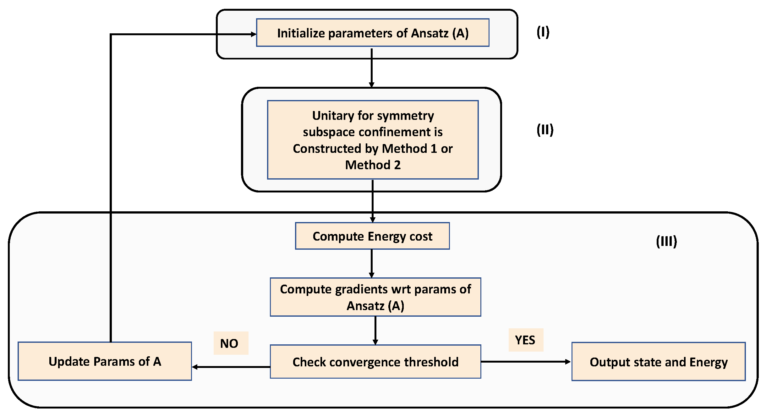
We schematically describe Method 2 in Figure 2b. In Figure 3, we describe an entire algorithm that is followed for both Method 1 and Method 2, and highlight the essential steps. Since we have discussed in detail the first two key steps of the algorithm, which includes preparation of the ansatz using $A(\overrightarrow{\alpha }){|0\rangle }^{⨂n}$ (see Figure 1) and operation of the unitary which confines the state within a symmetry subspace (see Figure 2), we emphasize in some detail the subsequent steps which articulate the procedure for obtaining the ground state energy in Figure 3 (designated as (III)). The procedure is similar to any variational hybrid algorithms routinely used nowadays. One computes the average energy using the Hamiltonian of the system and the parameterized state constrained in the symmetry sub-space (from step II in Figure 3). The gradient of this energy with respect to the parameters of the state is constructed and the convergence of the norm of the gradient is checked. If the desired threshold is not attained, parameters of the state are updated (by changing $\overrightarrow{\alpha }$ in step I in Figure 3) for the next iteration. The unitaries necessary to accomplish this operation come from the standard procedure of the conversion of the system Hamiltonian into Pauli-strings. The accompanying circuit description of such unitaries would then be highly specific to the system Hamiltonian.

3. Results

Both methods discussed above have been tested against $XXZ$ spin Hamiltonian and $H_2$ molecule Hamiltonian. We plot against chosen symmetries, the energy error, and state fidelity against the low energy state that respects the symmetry. The results have been obtained using Qiskit [23] state-vector simulator. The parameter updates in every iteration has been globally bound by 0.5 radians and reduced iteratively for convergence. The use of only $R_y$ and $R_x$ gates in our ansatz allows for gradients to be calculated with a shift of $\pi$ radians on the respective gate parameters, i.e., $d{R}_i(\theta )/d\theta =R_i(\theta +\pi )/2$, where $i\in x,y,z$.

3.1. $XXZ$ Spin Hamiltonian

The $XXZ$ spin Hamiltonian is given by,

$$H=\sum _{i}J({\sigma }_i^x{\sigma }_{i+1}^x+{\sigma }_i^y{\sigma }_{i+1}^y)+K{\sigma }_i^z{\sigma }_{i+1}^z$$

(7)

where the summation is over the nearest neighbour spins with open boundaries. We study the low energy states respected by the Reflection and Rotation Symmetry [24].

Both symmetry operators have eigenvalues of $\pm 1$. We would like to variationally probe the low energy states in each of these subspaces. We set the number of spins to be 4 and work with $J=1$ and $K=3$. This corresponds to 16 dimensional Hilbert space. For Method 2, we have made use of D = 5 layers as shown in Figure 2 to train the unitary $\tilde{U}(\overrightarrow{\theta })$ up to a mean error of 0.001 on the Symmetry value for 100 random samples generated by the ansatz $A(\overrightarrow{\alpha })$.

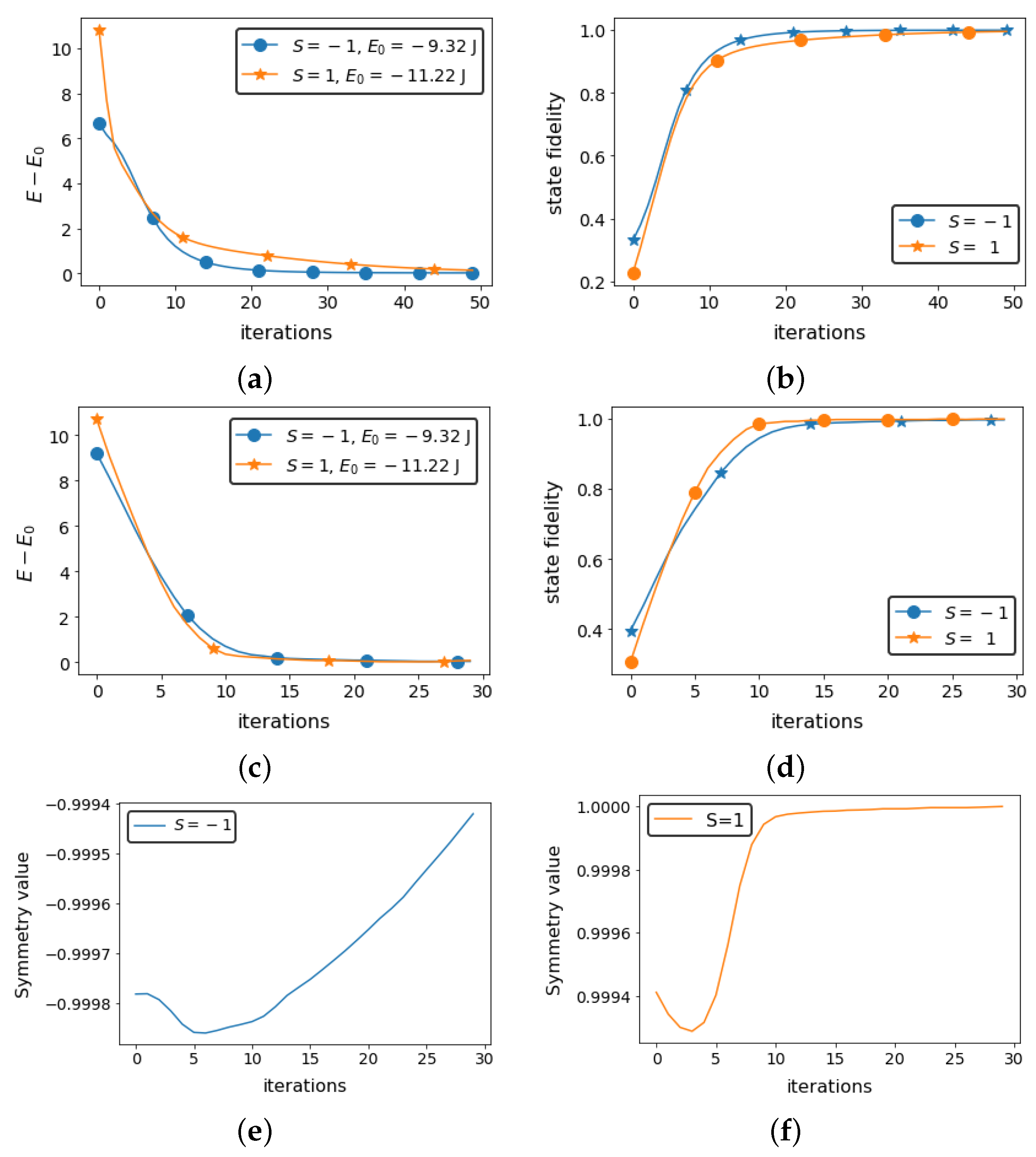
3.1.1. Reflection Symmetry

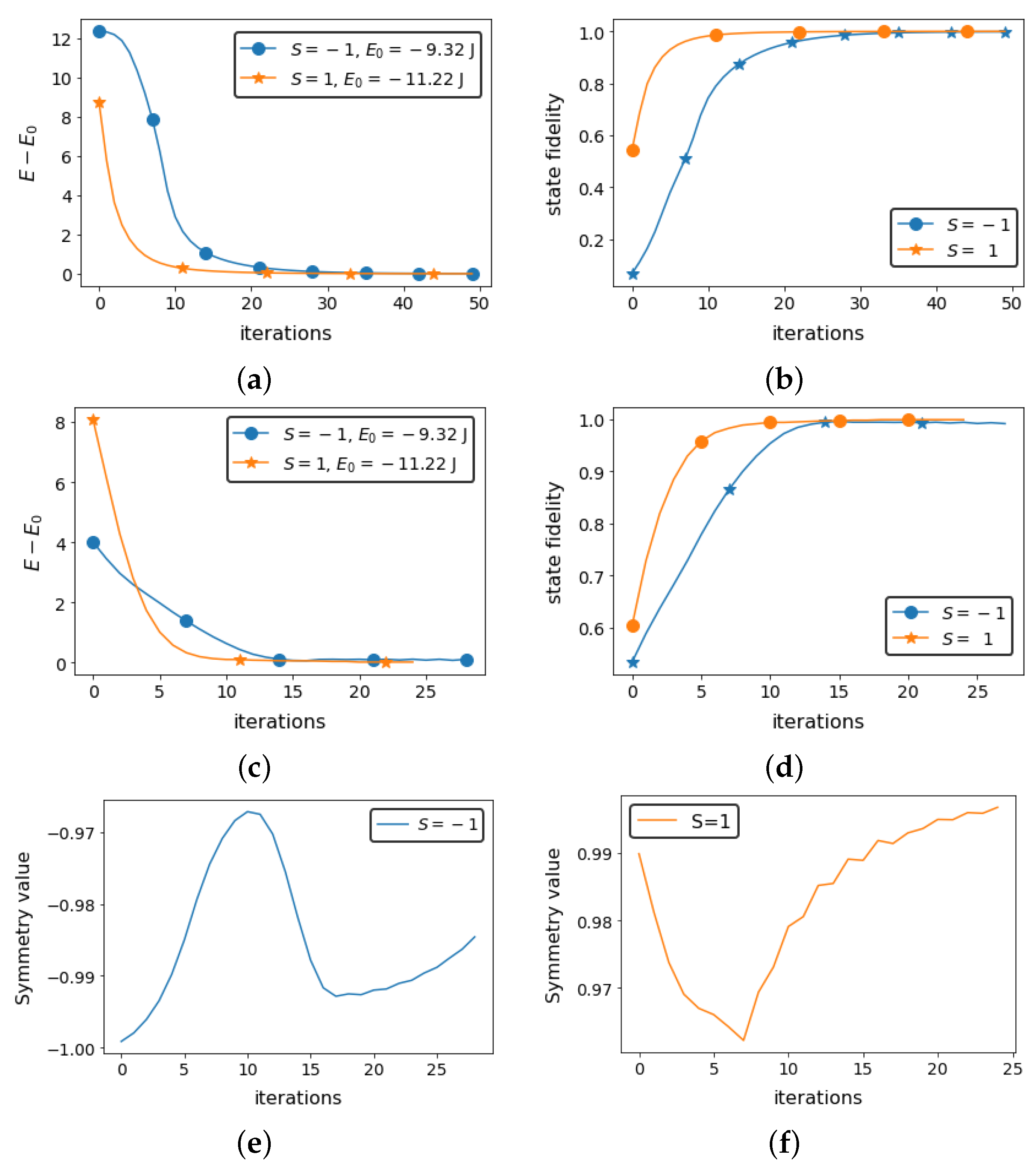
The reflection symmetry operator is given by $S={\Pi }_i({\sigma }_i^x{\sigma }_{i+1}^x+{\sigma }_i^y{\sigma }_{i+1}^y+{\sigma }_i^z{\sigma }_{i+1}^z+I)/2$ [24]. The reflection operator has a 6 dimensional subspace that measures -1 and a 10 dimensional subspace that measures +1. The decomposition of the Unitary was done through built in Qiskit modules that make use of isometry to optimize on the number of CNOT gates [25]. Figure 4 shows the energy error and state fidelity plots, indicating the convergence of the variational methods to the exact solution for each of the Symmetry values. Note that in Method 2, for $S=-1$, the method converges at the correct solution, despite the overall ground state energy being lower ($-11.226 J$). We notice that the symmetry value fluctuates within a very small interval around the exact value during the training.

3.1.2. Rotation Symmetry

The reflection symmetry operator is given by $S={\Pi }_i({\sigma }_i^x)$ [24]. The symmetry subspace of the rotation operator with eigenvalue $\pm 1$ is 8 dimensional. We use an exact decomposition of the unitary for Method 1 as presented in Appendix B. Figure 5 shows energy error and state fidelity plots indicating the convergence of the variational methods to the exact solution for each of the Symmetry values. Note that in Method 2, for $S=-1$, the method converges at the right solution, despite the overall ground state energy being lower (−11.226 J). Here again, we notice that the symmetry value fluctuates within a very small interval around the exact value during the training.

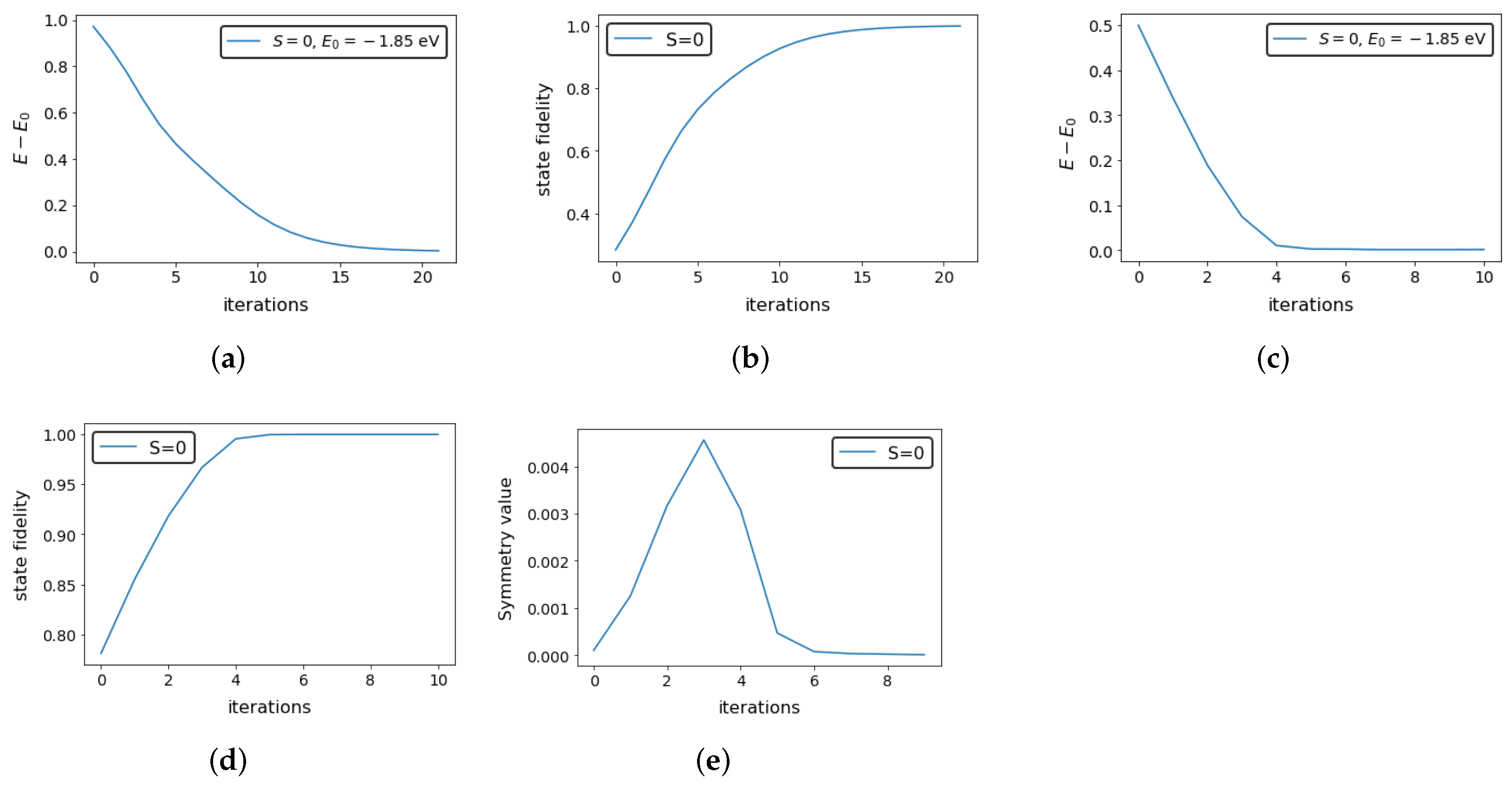
3.2. $H_2$ Hamiltonian

As an example of a real-molecular system, we chose the prototypical $H_2$ molecule. The electronic Hamiltonian for the system is constructed in the $STO-3G$ basis in the subspace spanned by vectors of the form |$n_2(\downarrow ),n_1(\downarrow ),n_2(\uparrow ),n_1(\uparrow )\rangle$ with ${\sum }_i{S}_z^i=0$ and $N={\sum }_i{a}_i^{†}{a}_i=2$ (the four such states are $|0110\rangle ,|0101\rangle ,|1010\rangle ,|1001\rangle$). The corresponding matrix (in units of eV) at the equilibrium bond length of 0.725 Å is [26]:

$$H=\left(\begin{array}{cccc}-1.06& 0& 0& 0.18\\ 0& -1.84& 0.18& 0\\ 0& 0.18& -0.23& 0\\ 0.18& 0& 0& -1.06\end{array}\right).$$

(8)

Since the entire space is spanned by states with the zero eigenvalue of ${\sum }_i{S}_z^i$, we have used the total angular momentum squared as the symmetry operator of our choice ($O_k={\widehat{S}}^2$). The latter operator in the aforesaid basis is given by,

$$S^2=\frac{1}{2}\left(\begin{array}{cccc}1.0& 0& 0& -1.0\\ 0& 0& 0& 0\\ 0& 0& 0& 0\\ -1.0& 0& 0& 1.0\end{array}\right).$$

(9)

Only one of the eigenvalues of the $S^2=s(s+1)$ matrix is 1 and the remaining ones are all 0. The techniques developed in this report requires the symmetry subspace to be of a dimension greater than 1. Therefore, we shall be restricting to the subspace $S^2=s(s+1)=0$. For Method 1, the unitary has been optimally decomposed using the KAK [27] decomposition algorithm. For Method 2, we have made use of D = 4 layers as shown in Figure 2 to train the unitary $U(\overrightarrow{\theta })$ up to a mean error of 0.001 on the Symmetry value for 100 random samples generated by the ansatz $A(\overrightarrow{\alpha })$. Figure 6 shows energy error and state fidelity plots indicating the convergence of the variational methods to the exact solution for $S^2=s(s+1)=0$. Here again, we notice that the symmetry value fluctuates within a very small interval around the exact value during the training.

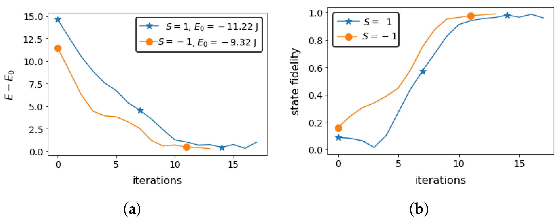
3.3. Simulation against Noise Models

We now test if the hardware efficient ansatz used results in a barren plateau, using noisy simulations for Method 1 for a 4 qubit $XXZ$ Hamiltonian with rotation symmetry. The simulation is done using Qiskit’s noise simulator with qubit properties listed in

Table 1. Details of the 4 qubit noise model sampled from Qiskit and used for simulating results shown in Figure 7. The noise model has been restricted to qubit errors only.

Qubit No.	T1 (us)	T2 (us)	Readout-Error (%)	Frequency (GHz)	Anharomonicity (GHz)
1	121.70	17.04	7.50	4.79	−0.31
2	111.68	132.02	2.24	4.94	−0.30
3	101.82	68.98	1.45	4.83	−0.31
4	116.71	85.88	2.15	4.80	−0.31

. No gate errors have been introduced. The method was run with no measurement error mitigation performed to validate the robustness. We see in Figure 7 that the energy values and state fidelity outputs fluctuate quite a bit in comparison to the results derived for noiseless simulations in the previous sections. We would like to point out that the ansatz $A(\overrightarrow{\alpha })$, being an hardware efficient ansatz, might have to be tuned so that the expressibility does not lead to vanishing gradients, as noted in [28].

4. Discussion

We discuss two general methods for restricting the exploration of a symmetry labelled subspace for a variational ansatz in identifying the ground state energy of a spin $XXZ$ Hamiltonian and $H_2$ Hamiltonian. Method 1 makes use of an exact unitary constructed from the symmetry operator, creating a large circuit decomposition. We overcome this through the use of variationally trained Unitaries developed in Method 2. The methods developed in here work more generally even when the constraint function does not commute with the Hamiltonian, i.e., is not a symmetry, as reflected in the construction of the unitary $\tilde{U}(\overrightarrow{\theta })$. We would also like to point out that Method 2 provides a useful tool for developing Unitaries variationally that satisfy a property of interest. The depth of the circuit and thus the number of parameters to be trained is likely to increase with the number of qubits. Additionally, it is possible to encounter symmetry operators in practice with eigenspaces that scales polynomially in the number of qubits. In such cases, hindrances in training due to barren plateaus are less likely to be encountered [29]. A proper size-dependant study can corroborate the assertion. Additionally, such studies may test the likelihood of the ansatz to be untrainable due to such restrictions and hence can serve as an insightful exercise to be undertaken in near future. As most symmetry operators of interest are usually defined with the similar operators acting over the entire qubit space, as future work one might want to investigate minimal 2 qubit unitaries that leave the Symmetry value unchanged and use them to create generalized ansatz over several qubits.

References

- Abrams, D.S.; Lloyd, S. Quantum Algorithm Providing Exponential Speed Increase for Finding Eigenvalues and Eigenvectors. Phys. Rev. Lett. 1999, 83, 5162–5165. [Google Scholar] [CrossRef] [Green Version]
- Nielsen, M.; Chuang, I.; Chuang, I. Quantum Computation and Quantum Information; Cambridge Series on Information and the Natural Sciences; Cambridge University Press: Cambridge, UK, 2000. [Google Scholar]
- Preskill, J. Quantum Computing in the NISQ era and beyond. Quantum 2018, 2, 79. [Google Scholar] [CrossRef]
- Peruzzo, A.; McClean, J.; Shadbolt, P.; Yung, M.H.; Zhou, X.Q.; Love, P.J.; Aspuru-Guzik, A.; O’Brien, J.L. A variational eigenvalue solver on a photonic quantum processor. Nat. Commun. 2014, 5, 4213. [Google Scholar] [CrossRef] [PubMed] [Green Version]
- Selvarajan, R.; Dixit, V.; Cui, X.; Humble, T.; Kais, S. Prime factorization using quantum variational imaginary time evolution. Sci. Rep. 2021, 11, 20835. [Google Scholar] [CrossRef] [PubMed]
- O’Malley, P.J.J.; Babbush, R.; Kivlichan, I.D.; Romero, J.; McClean, J.R.; Barends, R.; Kelly, J.; Roushan, P.; Tranter, A.; Ding, N.; et al. Scalable Quantum Simulation of Molecular Energies. Phys. Rev. X 2016, 6, 031007. [Google Scholar] [CrossRef] [Green Version]
- Lee, J.; Huggins, W.J.; Head-Gordon, M.; Whaley, K.B. Generalized Unitary Coupled Cluster Wave functions for Quantum Computation. J. Chem. Theory Comput. 2018, 15, 311–324. [Google Scholar] [CrossRef] [Green Version]
- Su, Y.; Huang, H.Y.; Campbell, E.T. Nearly tight Trotterization of interacting electrons. Quantum 2021, 5, 495. [Google Scholar] [CrossRef]
- Xia, R.; Kais, S. Quantum Machine Learning for Electronic Structure Calculations. Nat. Commun. 2018, 9. [Google Scholar] [CrossRef] [Green Version]
- Kandala, A.; Mezzacapo, A.; Temme, K.; Takita, M.; Brink, M.; Chow, J.M.; Gambetta, J.M. Hardware-efficient variational quantum eigensolver for small molecules and quantum magnets. Nature 2017, 549, 242–246. [Google Scholar] [CrossRef]
- Ryabinkin, I.G.; Genin, S.N.; Izmaylov, A.F. Constrained Variational Quantum Eigensolver: Quantum Computer Search Engine in the Fock Space. 2018. Available online: http://xxx.lanl.gov/abs/1806.00461 (accessed on 22 December 2021).
- Barkoutsos, P.; Gonthier, J.; Sokolov, I.; Moll, N.; Salis, G.; Fuhrer, A.; Ganzhorn, M.; Egger, D.; Troyer, M.; Mezzacapo, A.; et al. Quantum algorithms for electronic structure calculations: Particle/hole Hamiltonian and optimized wavefunction expansions. Phys. Rev. A 2018, 98, 022322. [Google Scholar] [CrossRef] [Green Version]
- Gard, B.T.; Zhu, L.; Barron, G.S.; Mayhall, N.J.; Economou, S.E.; Barnes, E. Efficient symmetry-preserving state preparation circuits for the variational quantum eigensolver algorithm. npj Quantum Inf. 2020, 6. [Google Scholar] [CrossRef]
- Nam, Y.; Chen, J.S.; Pisenti, N.C.; Wright, K.; Delaney, C.; Maslov, D.; Brown, K.R.; Allen, S.; Amini, J.M.; Apisdorf, J.; et al. Ground-State Energy Estimation of the Water Molecule on a Trapped Ion Quantum Computer. 2019. Available online: http://xxx.lanl.gov/abs/1902.10171 (accessed on 22 December 2021).
- Colless, J.I.; Ramasesh, V.V.; Dahlen, D.; Blok, M.S.; Kimchi-Schwartz, M.E.; McClean, J.R.; Carter, J.; de Jong, W.A.; Siddiqi, I. Computation of Molecular Spectra on a Quantum Processor with an Error-Resilient Algorithm. Phys. Rev. X 2018, 8, 011021. [Google Scholar] [CrossRef] [Green Version]
- McCaskey, A.J.; Parks, Z.P.; Jakowski, J.; Moore, S.V.; Morris, T.; Humble, T.S.; Pooser, R.C. Quantum Chemistry as a Benchmark for Near-Term Quantum Computers. 2019. Available online: http://xxx.lanl.gov/abs/1905.01534 (accessed on 22 December 2021).
- Shen, Y.; Zhang, X.; Zhang, S.; Zhang, J.N.; Yung, M.H.; Kim, K. Quantum implementation of the unitary coupled cluster for simulating molecular electronic structure. Phys. Rev. A 2017, 95. [Google Scholar] [CrossRef] [Green Version]
- Kuroiwa, K.; Nakagawa, Y.O. Penalty methods for a variational quantum eigensolver. Phys. Rev. Res. 2021, 3, 013197. [Google Scholar] [CrossRef]
- Sajjan, M.; Sureshbabu, S.H.; Kais, S. Quantum Machine-Learning for Eigenstate Filtration in Two-Dimensional Materials. J. Am. Chem. Soc. 2021, 143. [Google Scholar] [CrossRef]
- Schuld, M.; Bergholm, V.; Gogolin, C.; Izaac, J.; Killoran, N. Evaluating analytic gradients on quantum hardware. Phys. Rev. A 2019, 99. [Google Scholar] [CrossRef] [Green Version]
- Mitarai, K.; Negoro, M.; Kitagawa, M.; Fujii, K. Quantum circuit learning. Phys. Rev. A 2018, 98. [Google Scholar] [CrossRef] [Green Version]
- Mitarai, K.; Fujii, K. Methodology for replacing indirect measurements with direct measurements. Phys. Rev. Res. 2019, 1, 013006. [Google Scholar] [CrossRef] [Green Version]
- Aleksandrowicz, G.; Alexander, T.; Barkoutsos, P.; Bello, L.; Ben-Haim, Y.; Bucher, D.; Cabrera-Hernández, F.J.; Carballo-Franquis, J.; Chen, A.; Chen, C.-F.; et al. Qiskit: An Open-Source Framework for Quantum Computing. Zenodo 2019. [Google Scholar] [CrossRef]
- Joel, K.; Kollmar, D.; Santos, L.F. An introduction to the spectrum, symmetries, and dynamics of spin-1/2 Heisenberg chains. Am. J. Phys. 2013, 81, 450–457. [Google Scholar] [CrossRef] [Green Version]
- Iten, R.; Colbeck, R.; Kukuljan, I.; Home, J.; Christandl, M. Quantum circuits for isometries. Phys. Rev. A 2016, 93. [Google Scholar] [CrossRef] [Green Version]
- Zhang, F.; Gomes, N.; Berthusen, N.F.; Orth, P.P.; Wang, C.Z.; Ho, K.M.; Yao, Y.X. Shallow-circuit variational quantum eigensolver based on symmetry-inspired Hilbert space partitioning for quantum chemical calculations. Phys. Rev. Res. 2021, 3. [Google Scholar] [CrossRef]
- Nakajima, Y.; Kawano, Y.; Sekigawa, H. A New Algorithm for Producing Quantum Circuits Using KAK Decompositions. 2005. Available online: http://xxx.lanl.gov/abs/quant-ph/0509196 (accessed on 22 December 2021).
- Larocca, M.; Czarnik, P.; Sharma, K.; Muraleedharan, G.; Coles, P.J.; Cerezo, M. Diagnosing Barren Plateaus with Tools from Quantum Optimal Control. 2021. Available online: http://xxx.lanl.gov/abs/2105.14377 (accessed on 22 December 2021).
- Cerezo, M.; Sone, A.; Volkoff, T.; Cincio, L.; Coles, P.J. Cost function dependent barren plateaus in shallow parametrized quantum circuits. Nat. Commun. 2021, 12, 1791. [Google Scholar] [CrossRef] [PubMed]
Figure 1.
Ansatz () has been used to build the state within a k-dimensional space in Equation (2).
Figure 2.
The circuit decomposition and essential steps in (a) Method 1 and (b) Method 2.
Figure 3.
Flowchart indicating the steps involved in the algorithm. (I) Indicates preparation of the ansatz as illustrated in Figure 1. (II) Preparation of the unitary that dictates symmetry restriction as discussed in Figure 2. (III) The key steps in the variational optimization of the energy.
Figure 4.
Computing the lowest energy state of XXZ Hamiltonian within subspace labelled by the Reflection Symmetry Operator using Unitary constructed from method 1 and method 2. (a) Method 1: Energy error vs. iterations; (b) Method 1: State fidelity vs. iterations; (c) Method 2: Energy error vs. iterations; (d) Method 2: State fidelity vs. iterations; (e) Method 2: Symmetry value vs. iterations; (f) Method 2: Symmetry value vs. iterations.
Figure 5.
Computing the lowest energy state of XXZ Hamiltonian within subspace labelled by the Rotation Symmetry Operator using Unitary constructed from method 1 and method 2. (a) Method 1: Energy error vs. iterations; (b) Method 1: State fidelity vs. iterations; (c) Method 2: Energy error vs. iterations; (d) Method 2: State fidelity vs. iterations; (e) Method 2: Symmetry value vs. iterations; (f) Method 2: Symmetry value vs. iterations.
Figure 6.
Computing the lowest energy state of the hydrogen Hamiltonian within subspace labelled by using Unitary constructed from method 1 and method 2. (a) Method 1: Energy error vs. iterations; (b) Method 1: State fidelity vs. iterations; (c) Method 2: Energy error vs. iterations; (d) Method 2: State fidelity vs. iterations; (e) Method 2: Symmetry value vs. iterations.
Figure 7.
Computing the lowest energy state of XXZ Hamiltonian within subspace labelled by the Rotation Symmetry Operator using method 1 on a noisy Qiskit simulator. (a) Method 1: Energy error vs. iterations; (b) Method 1: State fidelity vs. iterations.