
Combined Remaining Life Prediction of Multiple Bearings Based on EEMD-BILSTM

1
School of Mines, China University of Mining and Technology, Xuzhou 221116, China
2
School of Industrial and Business Management, Xuzhou College of Industrial Technology, Xuzhou 221140, China
*
Author to whom correspondence should be addressed.
Symmetry 2022, 14(2), 251; https://doi.org/10.3390/sym14020251
Submission received: 31 October 2021
/
Revised: 10 December 2021
/
Accepted: 13 December 2021
/
Published: 27 January 2022
(This article belongs to the Special Issue Symmetry in Industrial Engineering)
Abstract
:To improve the accuracy of a symmetrical structural rolling bearing life prediction under noise interference, a multi-bearing life prediction method combining Ensemble Empirical Mode Decomposition (EEMD) and Bi-directional Long Short-Term Memory (BiLSTM) is proposed. First, EEMD is proposed to decompose the original vibration signal to obtain a finite number of Intrinsic Mode Function (IMF), and the IMFs are further filtered by combining the correlation criterion and kurtosis criterion. Then, the time domain features and frequency domain features of the reconstructed signal are filtered by monotonicity index to obtain the set of features containing key information. Finally, the BiLSTM network is trained on the filtered features set, and the method is proved to accurately predict the remaining life of rolling bearings under different operating conditions through rolling bearing full-life experiments, and the effectiveness of the method is verified by comparing the prediction results with several main recurrent neural networks.
1. Introduction
The functioning of rolling bearings, being the most significant component of rotating equipment, has a direct impact on the machine’s operation [1]. Extracting and modeling the rolling bearing symmetry characteristics is significant in improving remaining useful life prediction for mechanical equipment. The proactive maintenance of rolling bearings before they are damaged can effectively avoid accidents and thus reduce property losses. Therefore, it is important to study the prediction of its remaining life [2]. When it comes to the life prediction issue, multi-bearing synergetic analysis is more difficult since it considers many bearings with identical operating circumstances in order to determine the remaining life. Indeed, since the deterioration patterns of different bearings in a set might vary widely, it is difficult to accurately anticipate the remaining service life of numerous bearings at once [3].
The analysis of rolling bearing vibration signals has developed into the most efficient approach for monitoring bearing condition. On the one hand, there is typically noise interference in the bearing working environment, and the signal-to-noise ratio is poor. The measured vibration signal from numerous types of bearings, on the other hand, often exhibits nonlinearity. Fourier analysis and wavelet variation are often used in traditional fault analysis techniques. Fourier analysis is often used to deal with non-smooth data, although it has a low adaption rate. Wavelet transforms have multi-resolution properties, wavelet transform methods are sensitive to frequency mixing, wavelet basis selection is challenging, and wavelet transform algorithms are complex to develop. Empirical Mode Decomposition (EMD) is a time–frequency signal decomposition approach proposed by N.E. Huang [4] to analyze the non-smooth nonlinear signal. EEMD is a noise-assisted data analysis approach proposed by Z.Wu and N.E.Huang [5,6] to solve the mode mixing problem in view of the shortcomings of EMD method. A fault feature extraction approach based on EEMD was suggested by Lei [7], but did not give a filtering method for the Intrinsic Mode Function (IMF) component. Liu et al. [8] proposed the L-Kurtosis to filter the IMF components generated by EEMD decomposition.
Model-based approaches, knowledge-based methods, and data-driven methods are the three primary kinds of available methodologies for determining the remaining service life of bearings [9]. When the failure process is completely understood and the model parameters are successfully calculated, the physical model-based method delivers more accurate RUL estimations. Wang [10] suggested a mechanical condition prediction approach based on a probabilistic model and particle filtering. Lei [11] converted the PE model into an empirical model for predicting the remaining service life of machinery. However, as the complexity of contemporary mechanical systems grows, the failure causes of equipment become increasingly difficult to understand, making accurate and effective prediction techniques based on physical models increasingly challenging. With the rapid development of computer technology and sensor technology in recent years, massive amounts of mechanical data can be easily captured and stored, enabling a good collection of time series data generated during bearing operation. As a result, data-driven approaches for predicting bearing life have been effectively established. Deep learning methods’ development and implementation had a significant influence on the study of big data processing techniques [12]. Deep learning methods have high accuracy and large data processing capabilities, thus reducing modeling complexity [13]. RNN has been proven to be of a certain advantage in processing time series data due to its memory capability. LSTM and its derivatives, in particular, have been extensively used in picture captioning, voice recognition, genomic research, and natural language processing [14,15]. Zhao et al. [16] employed LSTM to assess tool wear condition. Malhotra et al. [17] introduced an Encoder-Decoder technique for Anomaly Detection (EncDec-AD) based on LSTM that learns to rebuild “normal” time-series behavior and then utilizes reconstruction error to identify abnormalities. Bruin [18] proposed LSTM networks to diagnose railroad track circuit fault in real time. As long as the LSTM model is fed a signal with a low sampling rate, it may provide decent results when used directly for processing. However, the vibration signals in the bearing prediction process are often with high-sampling-rate signals. Whenever an LSTM is applied immediately to a noisy signal, the model parameters are almost always excessively high and it is better to control the model, which may easily result in the unexpected result of overfitting. Furthermore, a regular LSTM can just recall data change features at the present moment. To this end, for the multi-bearing life prediction problem, an integrated prediction method based on EEMD noise reduction combined with BiLSTM [19] is designed and proposed in this paper. When compared to other approaches, the results of the trials reveal that the strategy is better in terms of enhancing prediction performance.
2. Problem and Methodology
2.1. Multi-Bearing Remaining Useful Life Co-Prediction
The majority of current research on rolling bearing life focuses on the individual bearings. However, different bearings have certain similarity in characteristics under the same working conditions, and machine learning algorithms can mine the characteristics of vibration data from vibration data well.
The challenge of forecasting the remaining service life of numerous bearings using condition monitoring data obtained under the same operating circumstances is known as cooperative prediction of the remaining service life of multiple bearings. Cooperative prediction of the remaining life of numerous bearings tries to forecast the remaining life of the bearings using both the bearings’ own monitoring data and the monitoring data for other bearings of the same kind and operating circumstances.
2.2. EEMD Noise Reduction Principle
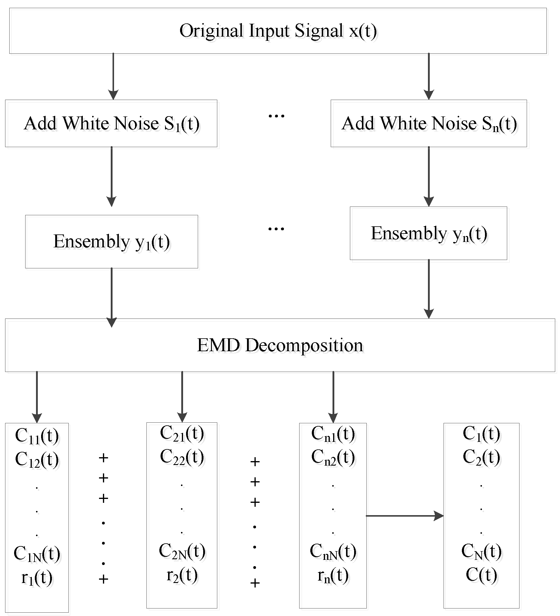
In recent years, as a successful approach for coping with nonlinear non-smooth signals, EMD has been able to deconstruct the signal into numerous IMFs, each of which reflects a component of each frequency in the original signal. This approach can address the issue of difficult basic function selection in wavelet noise reduction, but it cannot tackle the problem of noise-induced mode mixing [20]. Mode mixing refers to 1 IMF containing widely different characteristic timescales, or similar characteristic timescales distributed in different IMFs. In order to mitigate the mode mixing, Wu and Huang et al. [5] proposed an Ensemble Empirical Modal Decomposition (EEMD). EEMD is capable of adaptively separating the high frequency information in the fault signal well. The EEMD noise reduction method is shown in Figure 1:
- (1)
- A normally distributed white noise sequence is added to the collected signal to obtain , and normalize the noise-added signal.
- (2)
- The obtained signal is decomposed by EMD to obtain different IMFs and the residuals that represents the first noise is decomposed to obtain the first residual.
- (3)
- Repeat steps (1), (2) times and add a new random normally distributed white noise sequence each time.
- (4)
- The overall averaging operation of all decomposed obtained IMFs can eliminate the effect of adding white noise to the real IMF several times, and the final IMF components and residuals after EEMD decomposition are calculated as follows:where: is the EEMD decomposition of the first component and is the residual after decomposition.
- (5)
- Selection of IMF components: the decomposed components are listed in frequency order from high to low. When reconstructing the signal, the appropriate IMF components should be selected to retain the feature information to the maximum extent.
2.3. Principle of Bi-Directional Long and Short-Term Memory Network
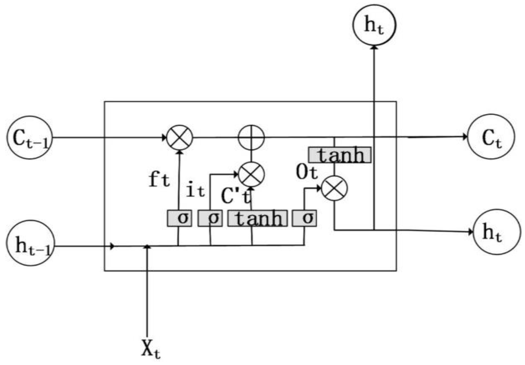
LSTM, as a particular case of RNN, not only avoids gradient explosion and disappearance, but also has a larger memory capacity than RNN, which has just one state h in the implicit layer that is sensitive to short-term input. The LSTM augments this with a long-term memory unit . As seen in Figure 2, the LSTM model is primarily responsible for controlling the memory unit c through three gate structures: an input gate, a forgetting gate, and an output gate [21].
The forgetting gate is primarily responsible for determining which information is forgotten at the final possible time. A number of (0, 1) is output by reading and . This value determines how much information will be retained by the cell state, with the formula:
The input gate’s primary duty is to contribute information to the cell’s state. The first section establishes values that are updated by the sigmoid function once the information is produced through the tanh activation function, as follows:
The update module status:
where, “∘” denotes the Hadamard Product. The output gate is in charge of determining whether or not to output the current state information, which is likewise formed of two sections: the first section is composed of , , and sigmoid activation. The second section includes the tanh activation function:
In the above equations, , and are linear correlation coefficients and bias coefficients, and is the sigmoid activation function.
The LSTM’s primary property is that each new input has some characteristics of the prior input. By regularly updating the model’s cellular state, the model retains long-term memory capacity.
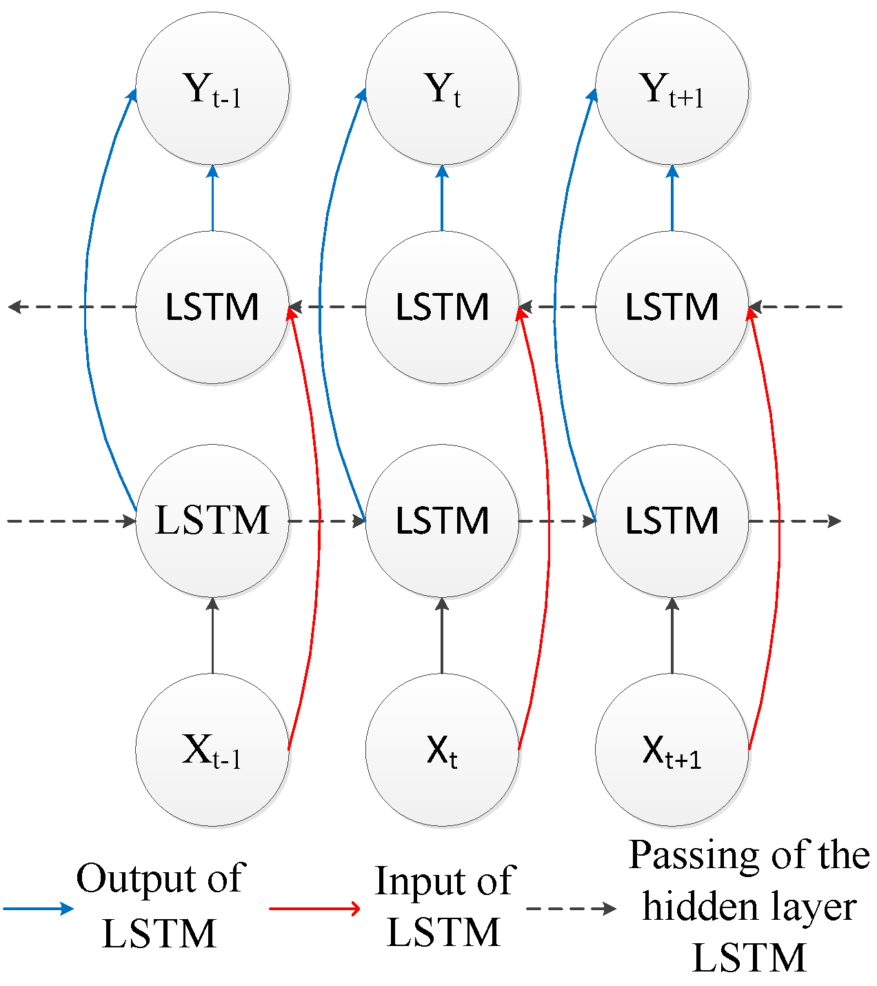
BiLSTM is made up of two LSTMs, one forward and one reverse, which could consider both past and future states by obtaining two time series with opposite hidden states and then connecting them to get the same output [22]. Therefore, BiLSTM can better grasp the complete information when processing time series data, and the BiLSTM structure is shown in Figure 3.
The hidden state of BiLSTM at moment contains the forward and backward
where: is the sequence length.
3. Methodological Steps
Three critical aspects must be considered in order to correctly anticipate the remaining life of rolling bearings.
① Filtering of the IMFs after EEMD decomposition. If the EEMD decomposition results are not selected, it may cause the extracted features to be vulnerable to noise interference. To accomplish noise reduction in this study, the correlation coefficient and kurtosis index are employed to filter the IMFs, and signal reconstruction is done on the filtered IMFs.
The correlation coefficient may be used to measure the degree of linear correlation between each IMF and the original signal, and it can be stated as:
where denotes the correlation coefficients for x and y. denotes the mathematical expectation, and are the mean values of the original signals and , and and are the standard deviations of the original signals and .
Kurtosis is a dimensionless parameter that can reflect the sharpness of the waveform. As can be seen from Equation (13), the kurtosis, as a fourth-order cumulative quantity, is unrelated to the size of the bearing, the rotational speed, or the load applied, but is very sensitive to the fault shock component of the signal,
where: N denotes the number of samples, is the standard deviation.
The correlation coefficient r is taken in the range (−1,1), and the interference of uncorrelated quantities in the vibration signal is reduced by finding the correlation coefficient of each IMF with the original signal. Normalize the desired kurtosis value and combine it with the desired correlation coefficient to define it as the value of IMF:
In Equation (14) and correspond to the kurtosis value and correlation coefficient of an IMF, and is the degree of the current IMF component’s kurtosis value on the weight of , and in this paper, we choose to be 0.6 through experiments.
② Analyzing the bearing state and choosing the best features. In this paper, a total of 13-time domain features and frequency domain features are extracted, among which some can well characterize the full life state of the bearing, while others cannot. In this research, monotonicity is used as a quantitative indicator to assess the extracted feature parameters quantitatively. The monotonicity index is calculated as follows:
In Equation (15): the feature signal sequence and the time series , the denotes the time at which corresponds to the eigenvalues at the time, is the total length of the sample time, and is the simple unit step function.
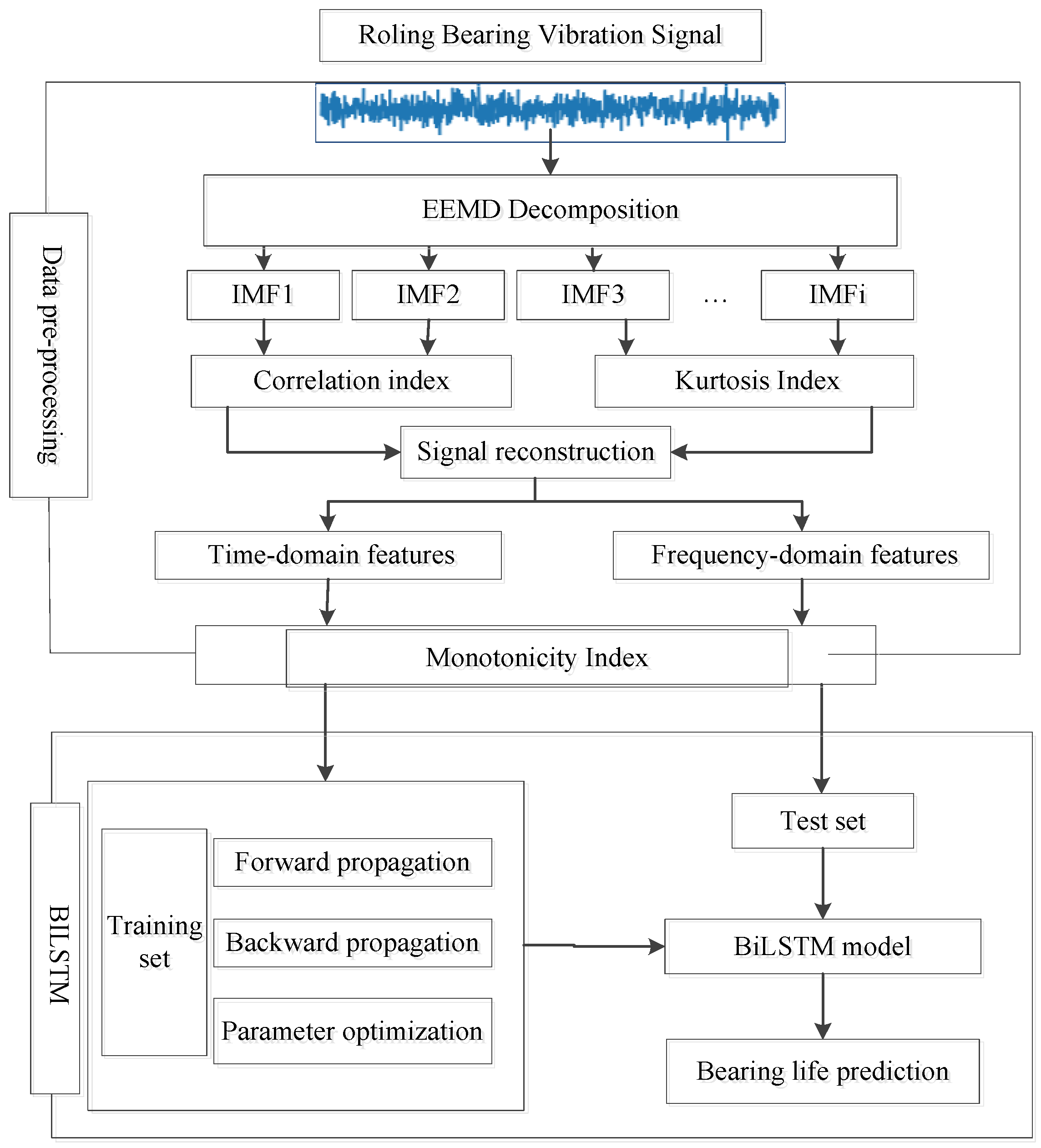
③ Selecting a suitable lifespan prediction model. The typical neural network predicts the remaining life using data from the present instant, and data volatility has a big influence on the prediction result, and it cannot understand the trend features of the data change with time well. The author presents a technique for predicting the remaining life of rolling bearings based on BiLSTM, and Figure 4 depicts the system’s flow chart. The following are the particular steps:
- (1)
- Filtering of IMFs: After EEMD decomposition of the original signal and obtaining a set of IMFs, the correlation coefficient of each IMF with the original signal is calculated according to Equation (12), the kurtosis value of each IMF is calculated according to Equation (13), and the of each IMF is calculated using Equation (14). For noise reduction, the IMF corresponding to the top three is chosen and rebuilt.
- (2)
- Extraction of feature parameters: The bearing’s full-life vibration data are used to extract the time and frequency domain features, and according to Equation (15), the features that do not accurately depict bearing deterioration are discarded, leaving the characteristics that do.
- (3)
- Determination of the degradation start moment point and define the network training label: Bearings are in normal operation for a long time throughout their lifetime, therefore we need to figure out where the degradation begins, and life forecast of their deterioration process may be a smart approach to conserve computing resources. In this paper, the degradation threshold is determined using μ + 3σ (μ is the median of the series and σ is the standard deviation of the series) [23]. The remaining life of the bearing is normalized to between (0, 1) from the moment of degradation to the complete failure of the bearing as the network prediction label.
- (4)
- BiLSTM network training and prediction: The whole lifespan of the first two bearings in each operational condition is utilized as the network’s training set, and the degraded feature set is used as the network’s input. The network is trained according to the labels so that the parameters of the network can be determined. The test bearing dataset is fed into the training network to validate the model’s accuracy and compare it to other algorithms.
- (5)
- Applicability of the model after training: Two evaluation metrics are provided to examine the performance of the test bearings on the model under various operating conditions by comparing the bearings under different operating conditions as a comparison.
4. Experiment Implementation
4.1. Data Description
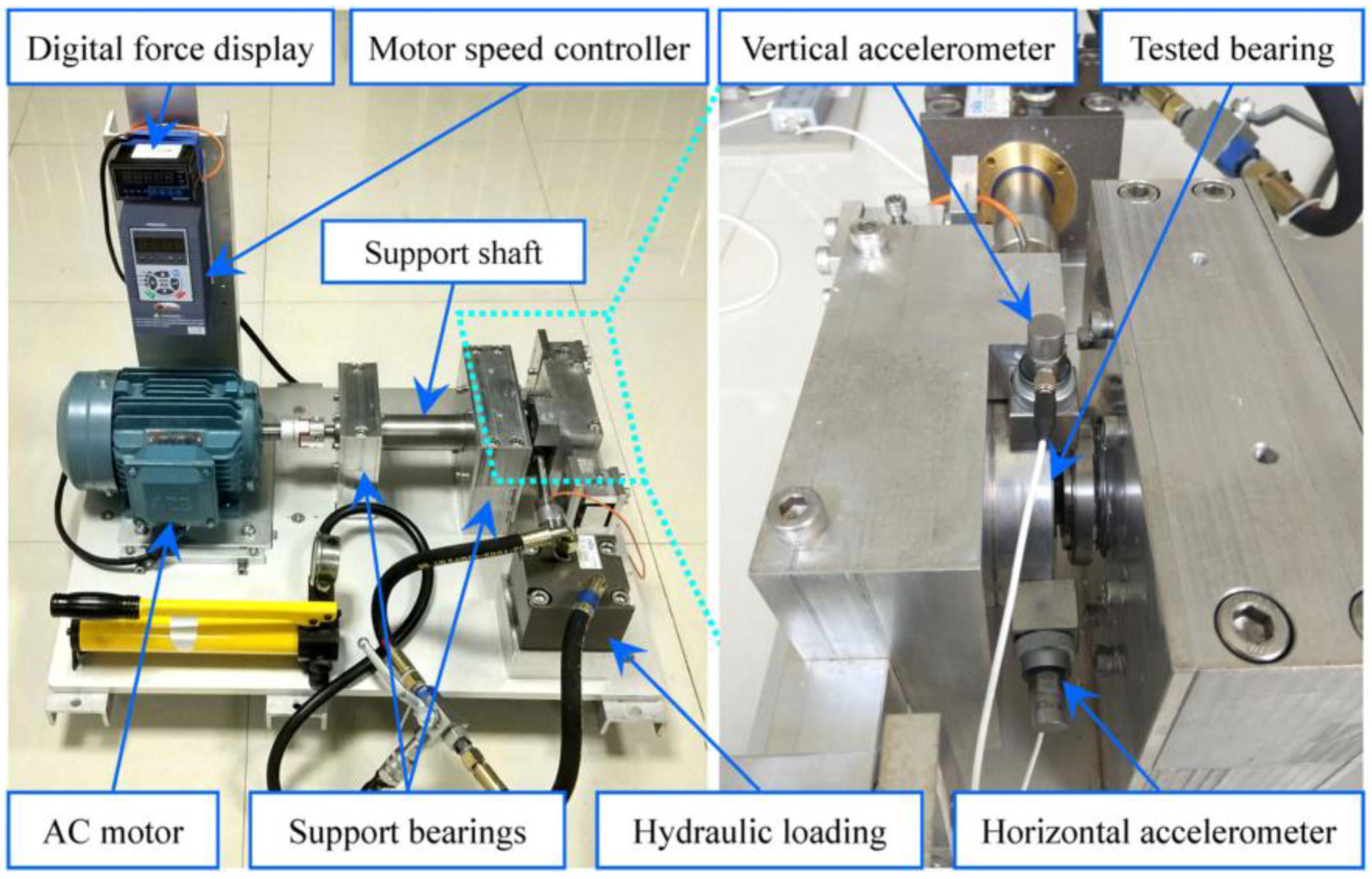
The XJTU-SY bearing data were used in this experiment and the specific experimental setup is shown in Figure 5. The purpose of the XJTU-SY test platform is to provide vibration signals throughout the service life of the naturally degraded bearing under different operating conditions. The rotational speed of the AC induction motor is controlled by the speed controller of the AC induction motor, which generates different radial forces that are applied to the tested bearing. The test is designed for three types of working conditions, and 5 samples are collected for each working condition of rolling bearing operation, and 15 samples in total for the three working conditions. They are named rolling bearing 1-1-rolling bearing 1-5, rolling bearing 2-1-rolling bearing 2-5, and rolling bearing 3-1-rolling bearing 3-5. Within each working condition, the first two bearings of each working condition are utilized as training samples, and the remaining three bearings of each working condition are employed as test samples in this experiment. Since the vertical vibration signals do not reflect the degradation information well, the horizontal vibration signals of the bearings are used for this study [24].
4.2. Sampling Point Setting
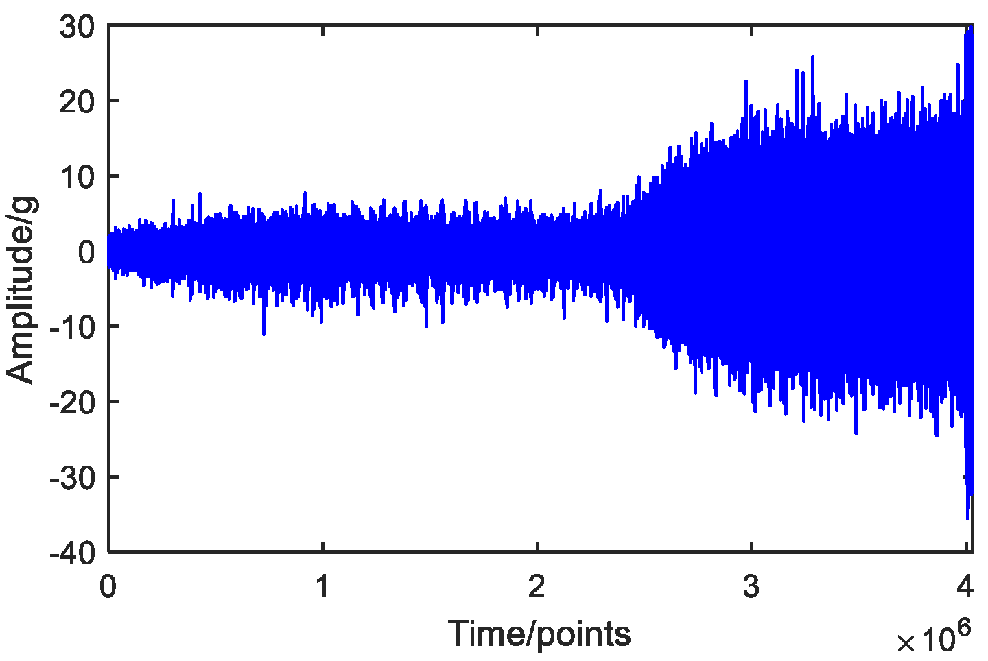
The sampling frequency in the experiment is 25.6 kHz while the length of each sample is 1.28 s, and the original signal is 32,768 sample points per group. In order to increase the experimental sample size, 4096 points were set as one sample in this study. The operating conditions of the rolling bearing under the three operating conditions are shown in Table 1. Figure 6 depicts the whole life signal of bearing 1-1.
5. Analysis of Results
5.1. EEMD Bearing Vibration Signal Noise Reduction
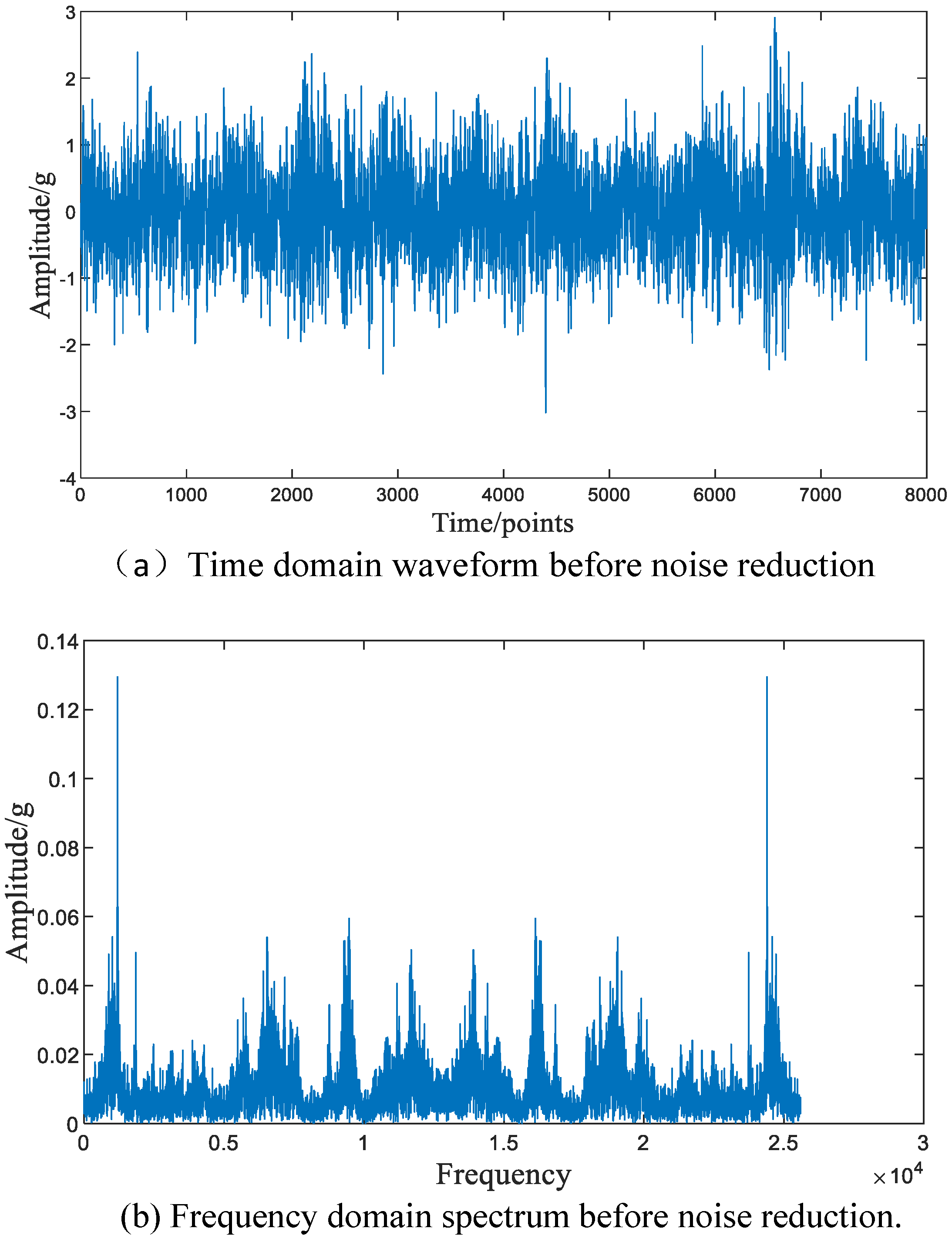
The data of a certain time period of the bearing are selected to verify the bearing noise reduction effect. The time–domain waveform and frequency spectrum of the bearing before noise reduction are presented in Figure 7, and the frequency spectrum shows that the initial vibration signal has a certain noise, which has a considerable interference to the bearing’s ability to extract useful information.
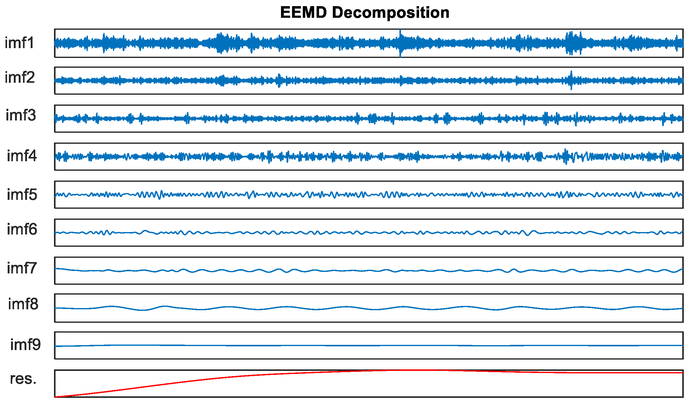
Next, the vibration signals of rolling bearings are processed for noise reduction by the EEMD method. In this paper, 100 groups of white noise sequences are added to the original signal . The amplitude of each group of white noise is set to 0.3, and a total of 9 IMFs and one residual are generated. Figure 8 shows the results of EEMD decomposition.
Then the correlation coefficients, kurtosis values, and values are calculated for each component, the first six IMFs are more correlated, but the kurtosis values of IMF1, IMF5, and IMF6 are smaller, and the results of values are shown in Table 2.
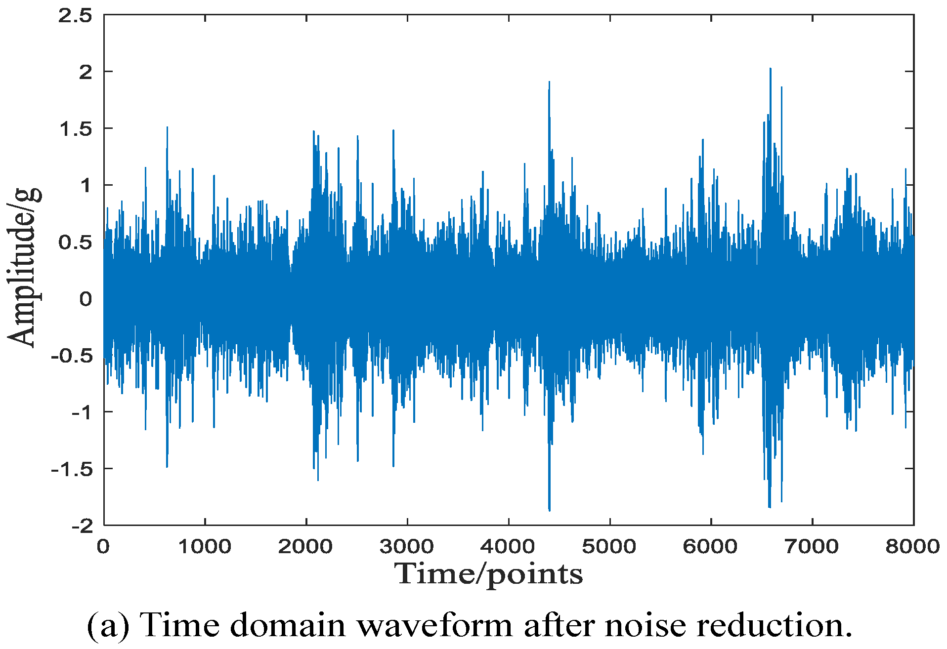
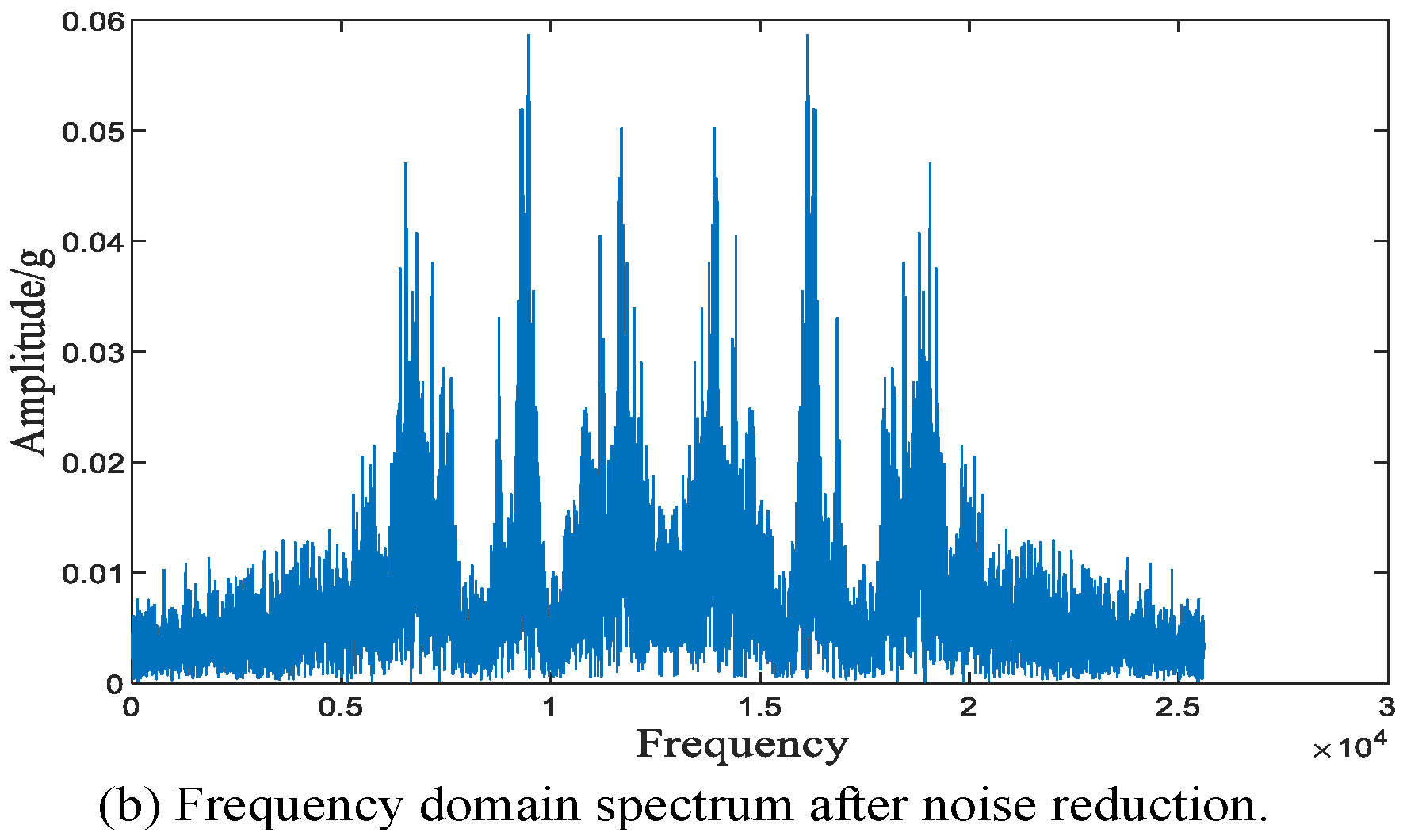
The values are sorted from largest to smallest, and the first three IMFs with larger values are selected for superposition to form the new vibration signal, and the selected components are IMF1, IMF3, and IMF4, and the other IMFs are rejected as noise. Figure 9 shows the time–domain waveform and frequency spectrum after noise reduction.
As can be seen in Figure 9, the low and high frequency components of the signal are weakened after noise reduction compared with the original signal, and the shock feature of the signal are more significant.
5.2. Feature Parameter Extraction
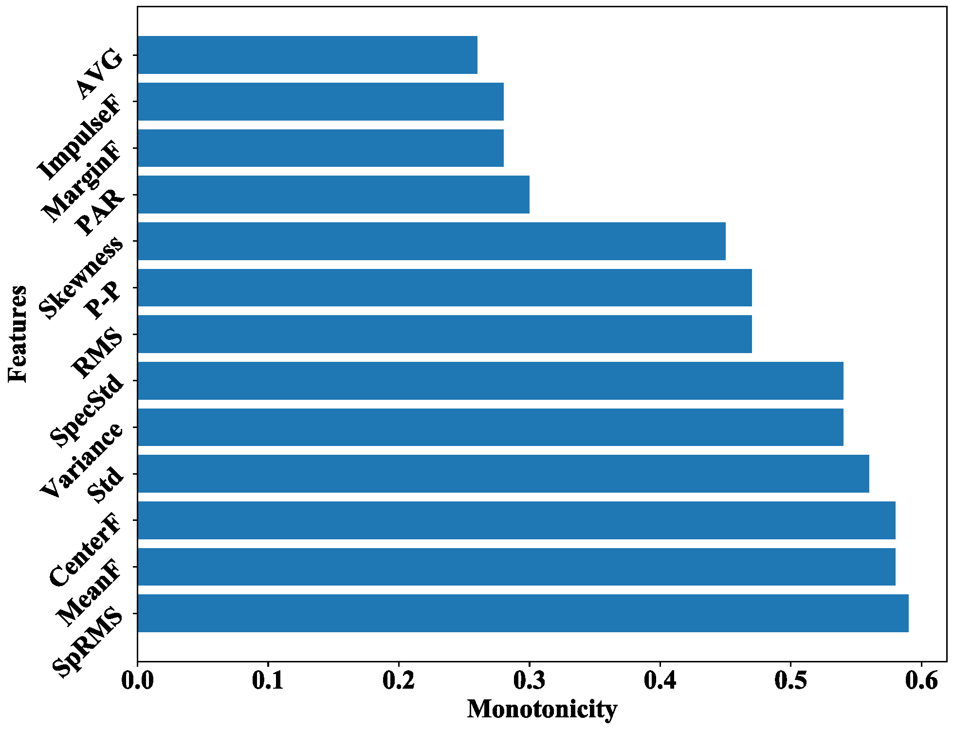
The full-life properties of rolling bearings are used to derive a total of 13 time–domain and frequency-domain features. The time–domain features are: Root Mean Square (RMS), Average Value (AVG), Skewness, Standard Deviation (Std), Variance, Peak-to-peak Value (P-P), Peak-to-average Ratio (PAR), Impulse Factor (ImpulseF), Margin Factor (MarginF). The frequency-domain features are: Frequency-domain Standard Deviation (SpecStd), Frequency-domain Root Mean Square (SpRMS), Frequency-domain Mean Frequency (MeanF), and Frequency-domain Center Frequency (CenterF).
It is proved that too many feature parameters can lead to an increase in the number of operations and result in long computation times. Fewer parameters may not reflect the bearing degradation trend better. In this paper, the monotonicity index is used to quantitatively filter out the feature parameters with strong characterization ability. The monotonicity can well reflect the time-series of the feature parameters, and the calculation is referred to Equation (15).
After quantification, the sorting results are shown in Figure 10, and the best result is obtained by testing that the threshold value of 0.5 is selected. The six features larger than the threshold value are extracted, and the normalization method is used to convert the extracted features to (0, 1) in order to eliminate the negative impact of different value ranges, which is then used as the input value of the life prediction model.
5.3. BiLSTM Lifetime Prediction
In this paper, we construct a BiLSTM model based on Keras, which provides various methods for initializing parameters based on probability distributions. A uniform distribution is generated as the initial weight initialization method. The first two layers use the sigmoid function as the activation function, while the ReLU function is chosen as the activation function for the Dence layer, where the optimizer is selected from Adam and Dropout technique is applied to prevent overfitting [23,25]. The network parameters of the BiLSTM are shown in Table 3.
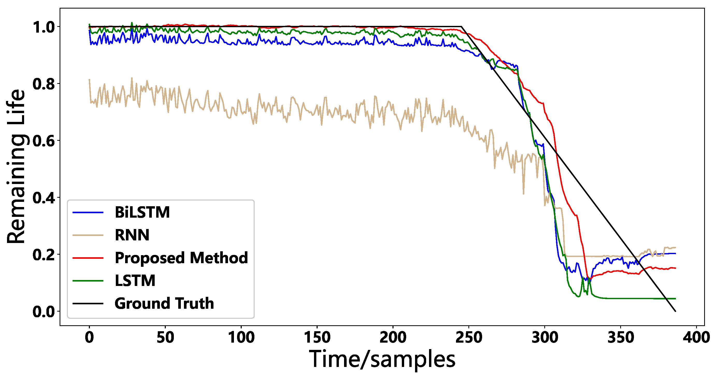
We performed a comparative experiment by using BiLSTM, LSTM, and RNN to validate the accuracy of the EEMD-BiLSTM remaining life prediction model. Because all recurrent networks have the same structure, the only thing that has to be changed is the kind of recurrent network, while the parametric network stays unaltered.
As shown in Figure 11, the full-life prediction results of bearing 1-4 under each model can predict the life degradation trend well, among which RNN is less effective since RNN has only one hidden state. Assuming that the bearing degrades at point t, the reason for the large prediction accuracy error at the time when the bearing first begins to degrade is that the bearing has just failed, and because the damage at point t is greater than at other locations, the vibration signal when the bearing is running to point t should be significantly different from the state at other points in the same rotation cycle, resulting in low prediction accuracy. As the bearing wears, the signal variation at point t becomes less noticeable compared to other places, and model’s accuracy improves. Therefore, the proposed method can better predict the remaining bearing life and provide for the effective operation of the bearings.
The Mean Absolute Error (MAE) and Root Mean Square Error (RMSE) assessment indices of the model are utilized in this paper to validate the applicability of the suggested method’s applicability. The two equations are shown as follows:
where: is the sample size of data, is the value of the th sample, and is the prediction value of the th sample.
Table 4 shows the results of a comparison of the prediction results with the commonly used time series algorithms. As shown in table, except for bearings 1-5 and 2-3, which have slightly higher prediction errors, all seven bearings perform well. 1-5 and 2-3 are due to bearing cage damage, and future research in this area can focus on life prediction using the proposed algorithm. The proposed method’s mean values for RMSE and MAE are 0.125 and 0.257, respectively, and the experimental results confirm the effectiveness of the proposed algorithm for lifetime prediction.
6. Conclusions
The remaining life of multiple bearings are studied based on combining model in this paper and the follows conclusions are drawn.
- (1)
- The ensemble empirical modal decomposition method is proposed and the decomposed IMFs are filtered by combining the correlation coefficient and the kurtosis index. It is proved that the final reconstructed signal can adequately remove the irrelevant noise.
- (2)
- Thirteen time-domain and frequency-domain features are extracted from the noise-reduced signal, and the initial feature set is filtered using monotonicity, and the feature set composed of the filtered features can fully retain the degradation information of the bearings.
- (3)
- The experimental analysis results show that the proposed method in this paper is more effective and has better prediction accuracy compared to other recurrent neural networks. It is more applicable and shows good performance in different working conditions.
Author Contributions
Conceptualization, Y.Z. and S.S.; methodology, S.S.; software, S.S. and F.W.; validation, X.L., Y.Z. and F.W.; formal analysis, Y.Z.; investigation, S.S.; resources, Y.Z.; data curation, S.S.; writing—original draft preparation, S.S.; writing—review and editing, X.L.; visualization, F.W.; supervision, X.L.; project administration, X.L.; funding acquisition, Y.Z. All authors have read and agreed to the published version of the manuscript.
Funding
This research was supported by the National Key Research and Development Project of China (grant no.: 2017YFC0804408).
Institutional Review Board Statement
Not applicable.
Informed Consent Statement
Not applicable.
Data Availability Statement
Not applicable.
Acknowledgments
The authors would like to acknowledge the support of the ShanDong Energy Group Xinglongzhuang coal mine.
Conflicts of Interest
The authors declare no conflict of interest.
References
- Tallian, T.E.; Gustafsson, O.G. Progress in rolling bearing vibration research and control. ASLE Trans. 1965, 8, 195–207. [Google Scholar] [CrossRef]
- Li, B.; Chow, M.-Y.; Tipsuwan, Y.; Hung, J.C. Neural-network-based motor rolling bearing fault diagnosis. IEEE Trans. Ind. Electron. 2000, 47, 1060–1069. [Google Scholar] [CrossRef] [Green Version]
- Ren, L.; Cui, J.; Sun, Y.; Cheng, X. Multi-bearing remaining useful life collaborative prediction: A deep learning approach. J. Manuf. Syst. 2017, 43, 248–256. [Google Scholar] [CrossRef]
- Huang, N.E.; Shen, Z.; Long, S.R.; Wu, M.C.; Shih, H.H.; Zheng, Q.; Yen, N.-C.; Tung, C.C.; Liu, H.H. The empirical mode decomposition and the Hilbert spectrum for nonlinear and non-stationary time series analysis. Proc. R. Soc. Lond. Ser. Math. Phys. Eng. Sci. 1998, 454, 903–995. [Google Scholar] [CrossRef]
- Huang, N.E.; Wu, Z. A review on Hilbert-Huang transform: Method and its applications to geophysical studies. Rev. Geophys. 2008, 46, RG2006. [Google Scholar] [CrossRef] [Green Version]
- Wu, Z.; Huang, N.E. Ensemble empirical mode decomposition: A noise-assisted data analysis method. Adv. Adapt. Data Anal. 2009, 1, 1–41. [Google Scholar] [CrossRef]
- Lei, Y.; He, Z.; Zi, Y. Application of the EEMD method to rotor fault diagnosis of rotating machinery. Mech. Syst. Signal Process. 2009, 23, 1327–1338. [Google Scholar] [CrossRef]
- Liu, H.; Xiang, J. A Strategy Using Variational Mode Decomposition, L-Kurtosis and Minimum Entropy Deconvolution to Detect Mechanical Faults. IEEE Access 2019, 7, 70564–70573. [Google Scholar] [CrossRef]
- Chen, Y.; Jin, Y.; Jiri, G. Predicting tool wear with multi-sensor data using deep belief networks. Int. J. Adv. Manuf. Technol. 2018, 99, 1917–1926. [Google Scholar] [CrossRef]
- Wang, J.; Gao, R.X.; Yuan, Z.; Fan, Z.; Zhang, L. A joint particle filter and expectation maximization approach to machine condition prognosis. J. Intell. Manuf. 2019, 30, 605–621. [Google Scholar] [CrossRef]
- Lei, Y.; Li, N.; Gontarz, S.; Lin, J.; Radkowski, S.; Dybala, J. A Model-Based Method for Remaining Useful Life Prediction of Machinery. IEEE Trans. Reliab. 2016, 65, 1314–1326. [Google Scholar] [CrossRef]
- Schmidhuber, J. Deep learning in neural networks: An overview. Neural Netw. 2015, 61, 85–117. [Google Scholar] [CrossRef] [PubMed] [Green Version]
- Deng, L. A dynamic, feature-based approach to the interface between phonology and phonetics for speech modeling and recognition. Speech Commun. 1998, 24, 299–323. [Google Scholar] [CrossRef]
- Bappy, J.H.; Simons, C.; Nataraj, L.; Manjunath, B.S.; Roy-Chowdhury, A.K. Hybrid LSTM and Encoder–Decoder Architecture for Detection of Image Forgeries. IEEE Trans. Image Process. 2019, 28, 3286–3300. [Google Scholar] [CrossRef] [Green Version]
- Auli, M.; Galley, M.; Quirk, C.; Zweig, G. Joint Language and Translation Modeling with Recurrent Neural Networks. In Proceedings of the 2013 Conference on Empirical Methods in Natural Language Processing, Washington, DC, USA, 18–21 October 2013; pp. 1044–1054. [Google Scholar]
- Zhao, R.; Wang, J.; Yan, R.; Mao, K. Machine health monitoring with LSTM networks. In Proceedings of the 2016 10th International Conference on Sensing Technology (ICST), Nanjing, China, 11–13 November 2016; pp. 1–6. [Google Scholar]
- Malhotra, P.; Ramakrishnan, A.; Anand, G.; Vig, L.; Agarwal, P.; Shroff, G. LSTM-based encoder-decoder for multi-sensor anomaly detection. arXiv 2016, arXiv:160700148. [Google Scholar]
- De Bruin, T.; Verbert, K.; Babuška, R. Railway track circuit fault diagnosis using recurrent neural networks. IEEE Trans. Neural Netw. Learn. Syst. 2016, 28, 523–533. [Google Scholar] [CrossRef]
- Graves, A.; Fernández, S.; Schmidhuber, J. Bidirectional LSTM Networks for Improved Phoneme Classification and Recognition. In Artificial Neural Networks: Formal Models and Their Applications—ICANN 2005, Proceedings of the 15th International Conference, Warsaw, Poland, 11–15 September 2005; Duch, W., Kacprzyk, J., Oja, E., Zadrożny, S., Eds.; Springer: Berlin/Heidelberg, Germany, 2005; pp. 799–804. [Google Scholar]
- Gao, Y.; Ge, G.; Sheng, Z.; Sang, E. Analysis and solution to the mode mixing phenomenon in EMD. In Proceedings of the 2008 Congress on Image and Signal Processing, Sanya, China, 27–30 May 2008; Volume 5, pp. 223–227. [Google Scholar]
- Gers, F.A.; Schraudolph, N.N.; Schmidhuber, J. Learning precise timing with LSTM recurrent networks. J. Mach. Learn. Res. 2002, 3, 115–143. [Google Scholar]
- Xu, G.; Meng, Y.; Qiu, X.; Yu, Z.; Wu, X. Sentiment Analysis of Comment Texts Based on BiLSTM. IEEE Access 2019, 7, 51522–51532. [Google Scholar] [CrossRef]
- Li, N.; Lei, Y.; Lin, J.; Ding, S.X. An Improved Exponential Model for Predicting Remaining Useful Life of Rolling Element Bearings. IEEE Trans. Ind. Electron. 2015, 62, 7762–7773. [Google Scholar] [CrossRef]
- Du, X.Q.; Yao, Z.H.; Chen, Z.C. Wavelet Denoising of the Horizontal Vibration Signal for Identification of the Guide Rail Irregularity in Elevator. Key Eng. Mater. 2007, 353–358, 2794–2797. [Google Scholar] [CrossRef]
- Hinton, G.E.; Srivastava, N.; Krizhevsky, A.; Sutskever, I.; Salakhutdinov, R.R. Improving neural networks by preventing co-adaptation of feature detectors. arXiv 2012, arXiv:1207.0580. [Google Scholar]
Figure 1.
EEMD decomposition steps.

Figure 2.
The architecture of a LSTM memory cell.

Figure 3.
The network structure of BiLSTM.

Figure 4.
Flowchart of the proposed method.

Figure 5.
The test platform of XJTU-SY.

Figure 6.
The full life vibration signal of bearing 1-1.

Figure 7.
Time–domain waveform and frequency spectrum of the raw signal.

Figure 8.
IMF component obtained by EEMD decomposition.

Figure 9.
Time–domain waveform and frequency spectrum of the reconstruction signal.


Figure 10.
The monotonicity index of features.

Figure 11.
Prediction result of bearing 1-4.


Table 1.
Bearing accelerated life test conditions.
| Work Condition Number | 1 | 2 | 3 |
|---|---|---|---|
| Speed/(r/min) | 2100 | 2250 | 2400 |
| Radial force/kN | 12 | 11 | 10 |
Table 2.
Values for the first six IMF components.
| IMF | IMF1 | IMF2 | IMF3 | IMF4 | IMF5 |
|---|---|---|---|---|---|
| Kρ | 0.576 | 0.791 | 0.733 | 0.685 | 0.463 |
Table 3.
BiLSTM model parameters.
| Network Type | Input Dimension | Output Dimensions | Activation Function | Dropout Rate |
|---|---|---|---|---|
| BiLSTM | (None,6,15) | (None,6,650) | Sigmiod | - |
| BiLSTM | (None,6,650) | (None,6,300) | Sigmiod | - |
| Dense_1 | (None,6,300) | (None,6,25) | Relu | 0.5 |
| Dense_2 | (None,6,25) | (None,6,1) | Relu | - |
Table 4.
Prediction error.
| Bearing | RNN | LSTM | BiLSTM | Proposed Method | ||||
|---|---|---|---|---|---|---|---|---|
| RMSE | MAE | RMSE | MAE | RMSE | MAE | RMSE | MAE | |
| 1-3 | 0.374 | 0.373 | 0.120 | 0.163 | 0.176 | 0.144 | 0.086 | 0.134 |
| 1-4 | 0.326 | 0.366 | 0.115 | 0.191 | 0.096 | 0.139 | 0.078 | 0.126 |
| 1-5 | 0.431 | 0.341 | 0.198 | 0.213 | 0.163 | 0.193 | 0.172 | 0.904 |
| 2-3 | 0.493 | 0.395 | 0.301 | 0.351 | 0.230 | 0.267 | 0.201 | 0.341 |
| 2-4 | 0.364 | 0.377 | 0.183 | 0.288 | 0.193 | 0.291 | 0.096 | 0.149 |
| 2-5 | 0.391 | 0.367 | 0.221 | 0.237 | 0.281 | 0.346 | 0.095 | 0.146 |
| 3-3 | 0.431 | 0.485 | 0.519 | 0.349 | 0.633 | 0.693 | 0.155 | 0.192 |
| 3-4 | 0.406 | 0.467 | 0.291 | 0.316 | 0.257 | 0.379 | 0.139 | 0.183 |
| 3-5 | 0.382 | 0.468 | 0.214 | 0.260 | 0.176 | 0.176 | 0.103 | 0.144 |
| Mean | 0.399 | 0.404 | 0.240 | 0.263 | 0.245 | 0.292 | 0.125 | 0.257 |
Publisher’s Note: MDPI stays neutral with regard to jurisdictional claims in published maps and institutional affiliations. |
© 2022 by the authors. Licensee MDPI, Basel, Switzerland. This article is an open access article distributed under the terms and conditions of the Creative Commons Attribution (CC BY) license (https://creativecommons.org/licenses/by/4.0/).
Share and Cite
MDPI and ACS Style
Zhan, Y.; Sun, S.; Li, X.; Wang, F. Combined Remaining Life Prediction of Multiple Bearings Based on EEMD-BILSTM. Symmetry 2022, 14, 251. https://doi.org/10.3390/sym14020251
AMA Style
Zhan Y, Sun S, Li X, Wang F. Combined Remaining Life Prediction of Multiple Bearings Based on EEMD-BILSTM. Symmetry. 2022; 14(2):251. https://doi.org/10.3390/sym14020251
Chicago/Turabian StyleZhan, Yujie, Song Sun, Xiangong Li, and Fuqi Wang. 2022. "Combined Remaining Life Prediction of Multiple Bearings Based on EEMD-BILSTM" Symmetry 14, no. 2: 251. https://doi.org/10.3390/sym14020251
Note that from the first issue of 2016, this journal uses article numbers instead of page numbers. See further details here.