
Symmetries and Solvability of a Class of Higher Order Systems of Ordinary Difference Equations


School of Mathematics, University of the Witwatersrand, Johannesburg 2050, South Africa
*
Author to whom correspondence should be addressed.
†
These authors contributed equally to this work.
Symmetry 2022, 14(1), 108; https://doi.org/10.3390/sym14010108
Submission received: 6 December 2021
/
Revised: 24 December 2021
/
Accepted: 5 January 2022
/
Published: 8 January 2022
(This article belongs to the Special Issue Recent Advances and Applications of Lie Symmetry Techniques)
Abstract
:We perform Lie analysis for a system of higher order difference equations with variable coefficients and derive non-trivial symmetries. We use these symmetries to find exact formulas for the solutions in terms of k. Furthermore, a detailed study for a specific value of k is presented. Our findings generalize some results in the literature.
1. Introduction
A Norwegian mathematician, Marius Sophus Lie (1842–1899) is responsible for the discovery of the transformations of variables and its properties. He began by investigating the continuous groups of transformations that would leave the differential equations invariant and his work created what is now known as symmetry analysis of differential equations. Lie’s original aim was to set a general theory for the integration of ordinary differential equations which was similar to the work that was done by Galois Abel [1] on algebraic equations in 1888. During the nineteenth century, Lie developed and applied the symmetry analysis of differential equations [2]. The theory that he developed enabled one to derive the solutions of differential equations in an algorithmic way that did not require any special guesses. There has been a lot of interest in the way Lie approached differential equations and notable mentions include the work done by Sedov Leonid Ivanovich [3] and Garrett Birkhoff [4] on the dimensional analysis. Their individual work proved to be important in the understanding of Lie’s approach to differential equations because they showed that Lie’s theory gave pertinent results in applied problems. Before this, there was a German mathematician Hermann Weyl (1885–1955) who in 1928 took interest in the abstract theory of Lie groups, and the term Lie group was coined by him in the same year. There has been a restoration of interest in Lie’s theory in recent decades and during these decades there has been a lot of crucial progress that was made from an applied point of view or a theoretical one. Lie’s theory involves a lot of tedious and cumbersome calculations. Lie group analysis has been and is still an essential tool in various fields like physics, number theory, differential equations, differential geometry, analysis and more.
Many researchers have investigated the application of Lie symmetry analysis to difference equations. Systematic algorithms and methods dealing with the derivation of symmetries for difference equations are now recorded and well documented. Some of the first works can be traced back to Maeeda [5,6] who developed an algorithm for obtaining continuous point symmetries of ordinary difference equations. Levi and Winternitz [7], Hydon [8], Quispel and Sahadeva [9], among others, have greatly contributed to the use of the Lie’s theory to difference equations.
Just like differential equations, difference equations have applications in real life (simple and compound interests, loan repayments, biological population dynamics, etc.). In general, difference equations are the perfect tools for describing phenomena that happen in discrete time steps. For example, in biological populations without overlapping generations, the growth of population takes place in discrete time steps and is modeled by difference equations (see [10]). An example of a typical model is that of semelparous populations which are insect populations with a single reproductive period before death. If we denote by the number of adults in the nth breeding time and the average number of eggs laid by an adult, the model turns out to be
for some constant t. See [10] for more details. Let denote the carrying capacity of the environment. Then, , and the model is known as the Beverton–Holt model [10]. Note that (1) implies that
where and .
In [11], the authors solved and dealt with the recursive equations:
where the real numbers and are the initial conditions.
In [12], the author determined and formulated the analytical solutions of the rational recursive equations:
where and are the initial conditions, which are arbitrary non-zero real numbers.
Note that appropriate change of variables transform equations in (3) and (4) into equations similar to (2).
The aim of this study is to generalize the results in [11,12] by studying the system of ordinary difference equations
where , , and are real sequences, using a symmetry method. Note that , , , are the initial conditions. For a similar work, see [13].
Understanding Lie groups and being able to use them is important because there is a lot that can be done with Lie groups, for example, we can get the Lie algebra action for a linear object by getting the derivative of the Lie group action. This is useful because when it comes to linear objects, it is much simpler to work with a Lie algebra than directly working with a Lie group. This is just one example of the many useful ways Lie groups can be used.
2. Preliminaries
In this section, we introduce some basic definitions and theorems needed in the work. Most of our definitions can be found in [8,14].
Definition 1.
A forward OΔE has the form
The domain D of the forward OE is said to be a regular domain if , . Here, the notation stands for .
Definition 2.
A parametrized set of point transformations,
where is a one-parameter local Lie group if the following conditions are satisfied:
- (1)
- is the identity map, so thatwhen
- (2)
- for every sufficiently close to zero.
- (3)
- Each can be represented as Taylor series in ε (in a neighborhood of that is determined by ), and therefore
Definition 3.
Consider with expand in Taylor series,
up to first order, we have
Definition 4.
A symmetry generator of (6) is denoted by U and is given by
where Q is the characteristic of the group of transformations.
In the above definition, . The operator S is known as the shift operator.
Consider the system of ordinary difference equations of the form
where the independent variable is n and the dependent variables are , and their shifts.
Consider the group of transformations
3. Symmetries and Solutions of the System of Difference Equations
Equivalently, Equation (5) can be written as
where , , and are real sequences. Applying (16) to (17) yields
After a set of long calculations, we get a system of determining equations for the characteristics and . Solving this system, we get
provided that
Using (21), we have that
The characteristic equation corresponding to (22) is giving by
Basically, r are the -th roots of 1, which are obtained as follows:
that is,
for any successive values of , say . This is the same as saying that
It follows that the solutions of (22) are given by
Using (21), we have that
Therefore (thanks to (14), (20), (27) and (28)), the system (17) has the following symmetry generators:
where . Thanks to (20), the canonical coordinates [15] are given by
Motivated by (21), we let and . For a better understanding, we use . We then get the invariants
Here, (31) is invariant under the group transformations of (20). In other words, the action of the symmetry generators, given in (29), on (31) gives zero. It is worthwhile mentioning that the symmetries together with the constraints on and have helped us to come up with the appropriate change of variables that will lead to the reduced system of equations. This is just one of the many roles of symmetries.
From (31), we get that
Performing iterations on (35), respectively, leads to the following:
where
The subscript of in (33) and (34) is where but the ones of in (36) are where . Therefore, we want to write in the form similar to We know that any positive integer r can be written as , , where denotes the remainder when r is divided by k. Hence,
and
Now, (37) and (38) are of the form similar to will either be 0 or 1. Substituting (37) and (38) into (36) leads to the following:
and
Back-shifting the equations above by k yields
and
for , 1, ⋯, . Equations (43) and (44) are the solutions of (5).
3.1. The Case When , , and Are Constant Sequences
3.2. A Detailed Study of the Case
One of the aims of this section is to verify the results in [11,12]. To achieve this, we substitute into (45) and (46). It yields the following:
and
where For the sake of clarity, we can rewrite (47) and (48) in expanded forms as follows:
Theorem 1.
The following system of equations
has a 2-periodic solution if , and , .
Proof.
Let and in the exact Equation (49). Then,
Following the same procedure as above on Equations ()–() gives and □
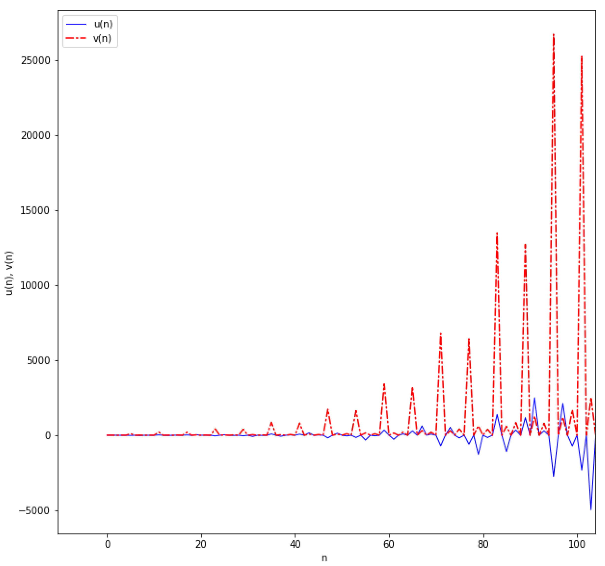
Below is a graph that illustrates the theorem above. Figure 1 is when we let and into the system of Equation (57).
Just as above, we similarly obtain the following:
In the above equation, we performed index shifting. Now,
Thus, (49) simplifies to
Following the same procedure as above, Equations ()–(), respectively, result in the following equations:
4. Conclusions
In this study, we looked at a system of th order ordinary difference equations. We investigated these equations by finding the symmetry generators (29). We then used the canonical coordinates to find the invariants in (31) of which led us to get the closed form solutions (33) and (34). Performing iterations resulted in (36), where we used the floor function definition and back-shifted the resulting equations to obtain the solutions (43) and (44) of (5). We performed a detailed study of the case where . The reason for studying this case is that we wanted to show that the work done in the articles [11,12] are special cases of our results. In fact, for different combinations of values of and D, which we get from the articles [11,12], we obtain the following important results:
Author Contributions
Both authors contribute equally to the manuscript. All authors have read and agreed to the published version of the manuscript.
Funding
This research received no external funding.
Institutional Review Board Statement
Not applicable.
Informed Consent Statement
Not applicable.
Data Availability Statement
Not applicable.
Conflicts of Interest
The authors declare no conflict of interest.
References
- Quadling, D.; Klein, F.; Lie, S. Evolution of the idea of symmetry in the nineteenth century, by IM Yaglom. Translated by Sergei Sossinsky and edited by Hardy Grant and Abe Shenitzer. Math. Gaz. 1988, 72, 341–342. [Google Scholar] [CrossRef]
- Lie, S. Vorlesungen über Differentialgleichungen: Mit Bekannten Infinitesimalen Transformationen; BG Teubner: Leipzig, Germany, 1891. [Google Scholar]
- Sedov, L.I.; Volkovets, A.G. Similarity and Dimensional Methods in Mechanics, 10th ed.; CRC Press: Boca Raton, FL, USA, 1961. [Google Scholar]
- Birkhoff, G. Hydrodynamics, a study in logic, fact, and similitude. Bull. Am. Math. Soc. 1951, 57, 497–499. [Google Scholar]
- Maeda, S. The similarity method for difference equations. IMA J. Appl. Math. 1987, 38, 129–134. [Google Scholar] [CrossRef]
- Maeda, S. Canonical structure and symmetries for discrete systems. Math. Jpn. 1980, 25, 405–420. [Google Scholar]
- Levi, D.; Winternitz, P. Continuous symmetries of discrete equations. Phys. Lett. A 1991, 152, 335–338. [Google Scholar] [CrossRef]
- Hydon, P.E. Difference Equations by Differential Equation Methods; Cambridge University Press: Cambridge, UK, 2014. [Google Scholar]
- Quispel, G.; Sahadeva, R. Lie symmetries and the integration of difference equations. Phys. Lett. A 1993, 184, 64–70. [Google Scholar] [CrossRef]
- Banasiak, J. Mathematical Modelling in One Dimension: An Introduction via Difference and Differential Equation; Cambridge University Press: Cambridge, UK, 2013. [Google Scholar]
- Almatrafi, M.B.; Elsayed, E.M. Solutions and formulae for some systems of difference equations. MathLAB J. 2018, 1, 356–369. [Google Scholar]
- Almatrafi, M.B. Analysis of Solutions of Some Discrete Systems of Rational Difference Equations. J. Comput. Anal. Appl. 2020, 29, 355–368. [Google Scholar]
- Folly-Gbetoula, M.; Nyirenda, D. A generalised two-dimensional system of higher order recursive sequences. J. Differ. Equ. Appl. 2020, 26, 244–260. [Google Scholar] [CrossRef]
- Hydon, P.E. Symmetry Methods for Differential Equations: A Beginner’s Guide; Cambridge University Press: Cambridge, UK, 2000; Volume 22. [Google Scholar]
- Joshi, N.; Vassiliou, P. The existence of Lie Symmetries for First-Order Analytic Discrete Dynamical Systems. J. Math. Anal. Appl. 1995, 195, 872–887. [Google Scholar] [CrossRef] [Green Version]
Figure 1.
Plof of .

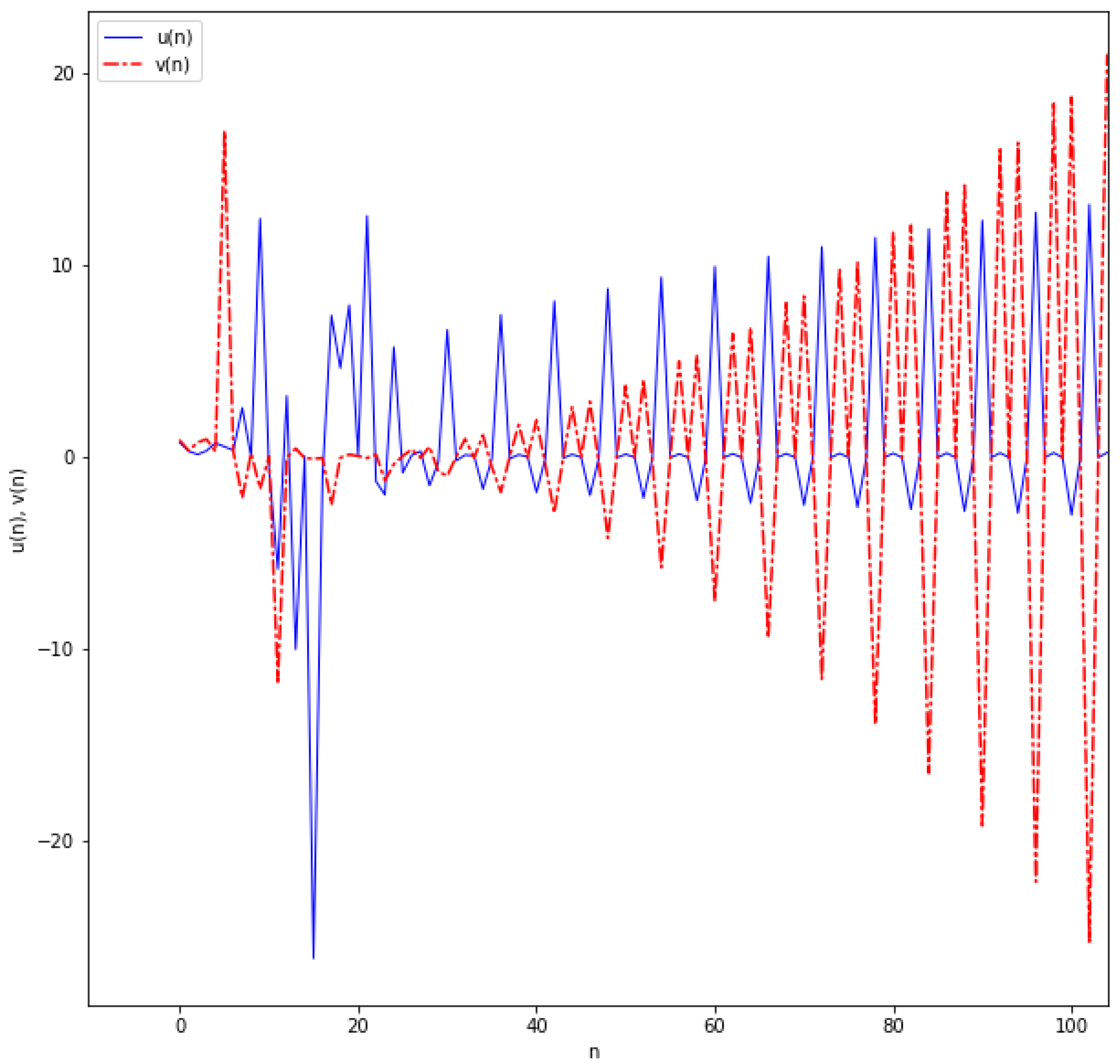
Figure 2.
Plot of .

Figure 3.
Plot of .

Publisher’s Note: MDPI stays neutral with regard to jurisdictional claims in published maps and institutional affiliations. |
© 2022 by the authors. Licensee MDPI, Basel, Switzerland. This article is an open access article distributed under the terms and conditions of the Creative Commons Attribution (CC BY) license (https://creativecommons.org/licenses/by/4.0/).
Share and Cite
MDPI and ACS Style
Mkhwanazi, K.; Folly-Gbetoula, M. Symmetries and Solvability of a Class of Higher Order Systems of Ordinary Difference Equations. Symmetry 2022, 14, 108. https://doi.org/10.3390/sym14010108
AMA Style
Mkhwanazi K, Folly-Gbetoula M. Symmetries and Solvability of a Class of Higher Order Systems of Ordinary Difference Equations. Symmetry. 2022; 14(1):108. https://doi.org/10.3390/sym14010108
Chicago/Turabian StyleMkhwanazi, Kgatliso, and Mensah Folly-Gbetoula. 2022. "Symmetries and Solvability of a Class of Higher Order Systems of Ordinary Difference Equations" Symmetry 14, no. 1: 108. https://doi.org/10.3390/sym14010108
Note that from the first issue of 2016, this journal uses article numbers instead of page numbers. See further details here.