An Interferometric Method for Particle Mass Measurements

Abstract

We present an interferometric method suitable to measure particle masses and, where applicable to the particle and its corresponding antiparticle, their mass ratio in order to detect possible symmetry violations between matter and antimatter. The method is based on interferometric techniques tunable to the specific mass range of the particle under consideration. The case study of electron and positron is presented, following the recent observation of positron interferometry.

1. Introduction

A great deal of effort is devoted to measuring the masses of particles or antiparticles as accurately as possible. Examples are given by the most recent mass evaluation of electron [1,2], proton [3], and antiproton [4]. These measurements are in general based on spectroscopic methods on ions or elementary particles confined in Penning trap systems.

In particular, the mass of a particle and its own antiparticle is predicted to be the same under the very general assumptions of the CPT theorem [5]. Measuring a mass difference would in fact imply a violation of the charge, parity, and time (CPT) reversal symmetry, which is one of the cornerstones of modern particle physics and quantum theory. The CPT theorem was demonstrated in 1957 [6] and is valid for relativistic quantum fields in a flat spacetime. A quantum field theory does not allow CPT violation without also admitting some level of violation of Lorentz Invariance [7]. Quantum Gravity models, however, predict the possibility of CPT violation at some level [8] due to effects at the Planck energy scale.

The most accurate evaluation of the relative mass difference between positron and electron (<$8\times {10}^{-9}$) is based on positronium spectroscopy, under the assumption that the positronium Rydberg constant is exactly half the hydrogen one [9]. A much more stringent limit (<$4\times {10}^{-23}$) is obtained from a theoretical argument based on the fact that any mass difference between electron and positron would lead to a non-zero photon mass [10,11]. The most accurate measurement of the relative mass difference between proton and antiproton is based on the spectroscopy of antiprotonic helium [12] and on antiproton charge-to-mass ratio constraints [13]. The comparison of the antiproton-to-proton charge-to-mass ratio with the highest accuracy so far is reported in [14].

Here, we propose a method for measuring the mass of a particle or of an antiparticle using the same setup. The technique is inspired by the interferometric measurement [15,16] that has demonstrated for the first time antimatter interference. The attainable accuracy on the mass is much lower than that obtained using Penning traps, but the proposed method is relatively simple, and it allows a direct measurement of the mass of an antiparticle that is not based on the comparison of particle/antiparticle charge-to-mass ratios. The used method explicitly assumes Lorentz invariance.

2. The Method

The proposed method is based on interferometry as a tool for mass (or mass ratio) measurements of particles and antiparticles. The interferometer can be considered (for given geometrical parameters) as a spectrometer whose task is measuring the de Broglie wavelength of the particle. The mass of the particle is then calculated by inverting the de Broglie relation. Namely, the de Broglie wavelength [17] is defined as $\lambda =h/p,$ where h is the Planck’s constant and p is the relativistic particle momentum. Denoting with K the particle kinetic energy, one has

$$\lambda =\frac{h}{mc\sqrt{{(1+K/m{c}^2)}^2-1}},$$

(1)

with c the speed of light and m the rest mass of the particle. Inverting the previous relation in terms of the rest energy, one obtains

$$m{c}^2=\frac{{(hc/\lambda )}^2-K^2}{2K}.$$

(2)

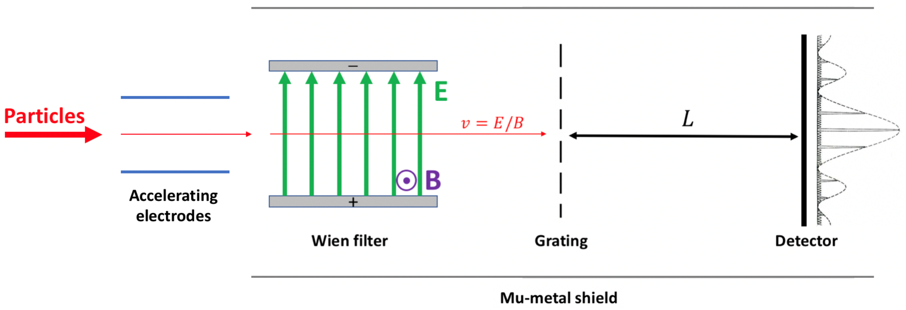
In a possible proposed configuration (see Figure 1) the kinetic energy of the particles is determined by an acceleration stage. The uncertainties on K are influenced in general by the initial velocity distribution of the particles and by the uncertainty on the potentials applied along the acceleration beamline.

In order to reduce the kinetic energy spread, a suitable (combination of) Wien filter(s) may be introduced (see again Figure 1). A Wien filter is a device consisting of orthogonal electric and magnetic fields, such that the Lorentz force for charged particles traveling with a velocity $v=E/B$ orthogonal to both fields vanishes, so that the trajectory of these particles is unaffected while all other particles are deflected [18,19]. For the present purposes, we assume that the $E/B$ ratio is adjustable around the expected velocity value:

$$\frac{E}{B}=v=c{\left[1-\frac{1}{{(1+K/m{c}^2)}^2}\right]}^{1/2}.$$

(3)

The actual velocity at the exit from the Wien filter could then be selected as that which maximizes the output particle flux (and therefore the statistics for the subsequent analysis). This can be determined with a suitable detector on the optical axis of the filter just after the exit. The drawback is that this velocity is known within the uncertainties of the electric and magnetic fields inside the filter. The advantage is that these uncertainties can be much smaller than the uncertainty on K in the previous acceleration stage; moreover, these uncertainties become completely unimportant in a mass ratio estimate (see later). Pinholes after the exit from the Wien filter may further collimate the beam before the interferometric stage.

In order to estimate the mass of a particle/antiparticle or the mass ratio of a particle and its corresponding antiparticle, a Fraunhofer diffraction configuration is considered (see Figure 1), with the goal of measuring the de Broglie wavelength of the particles.

Fraunhofer (far-field) diffraction occurs when the distance between the source and the diffraction object, as well as the distance between the diffraction object and the screen, is very large when compared with the wavelength of the incident wave.

A beam of particles with de Broglie wavelength $\lambda$ impinging on the slit system (or grating) generates an interference and diffraction pattern that appears as an intensity modulation when observed on a plane located at a distance L from the grating and is observed by recording the flux of particles as a function of the lateral screen position with a position-sensitive detector.

The intensity (normalized over its maximum value) is given by

$$\frac{I}{I_{max}}={\left(\frac{sin\beta }{\beta }\right)}^2\frac{{sin}^{2}N\alpha }{{sin}^2\left(\alpha \right)},$$

(4)

where N is the number of slits, $\beta =(\pi a/\lambda )sin\theta$, and $\alpha =(\pi d/\lambda )sin\theta$, with a the width of the slits, d the distance between (the centers of) successive slits, and $tan\theta =y/L$. Here, y denotes the lateral position on the screen ($y=0$ where the optical axis of the apparatus intercepts the screen).

Mathematically, the overall diffraction pattern is equivalent to that produced by N delta function (infinitesimal width) slits modulated by the intensity pattern of a single slit with finite width. The slit width a determines the distance between the minima of the diffraction envelope, whereas the separation d between the slits determines the distance between the minima of the interference pattern.

Here, we explicitly consider the use of a diffraction grating. The main advantage of this configuration over a diffracting system with a small number of slits is related to the reduced loss of particle statistics, which can represent an important problem especially when working with antimatter particles. For this same reason, the use of large opening slits is envisaged ($a=d/2$). A further advantage of the diffraction grating is the fact that by increasing N the principal maxima become more intense (as the intensity scales with $N^2$), their full width at half maximum becomes smaller and smaller and their position tends to become independent from the width of the slit a and given by the simple and well-known formula

$$sin{\theta }_n=n\lambda /d.$$

(5)

The position of the first lateral interference maxima therefore correspond to a deviation from the center of the screen of

$$\left|\mathsf{\Delta }y\right|=Ltan[arcsin(\lambda /d\left)\right].$$

(6)

Inverting this relation

$$\frac{\lambda }{d}=\frac{\left|\mathsf{\Delta }y\right|/L}{\sqrt{1+{\left(\right|\mathsf{\Delta }y|/L)}^2}},$$

(7)

and inserting this result in the definition of the de Broglie wavelength (2), one obtains

$$m{c}^2=\frac{hc}{d}\sqrt{\frac{c^2{B}^2}{E^2}-1}\sqrt{1+{\left(\frac{L}{\left|\mathsf{\Delta }y\right|}\right)}^2}.$$

(8)

This formula gives the absolute mass of the particle in our proposed approach. The error on the mass therefore depends on the errors relevant to the electric (E) and magnetic (B) fields in the velocity selector, the distance L between grating and screen, the grating pitch d, and the distance $\left|\mathsf{\Delta }y\right|$ between the central and first lateral interference maxima (average distance of the first maxima on both sides). In order to evaluate this error in a possible real experiment, we consider here the case of nuclear emulsion detectors [20,21,22]. In this case, the intrinsic resolution can reach 50 nm [23,24].

To estimate the particle statistics needed to reach a given resolution (this issue can be of critical importance in the case of antimatter particles), we have performed a simple Monte Carlo simulation. The events are randomly extracted according to the theoretical distribution (4) and are plotted in a histogram with the bin width equal to the expected resolution of the detector. As the error analysis indicates (see later) that the overall accuracy of the measurement is strongly affected by the accuracy on $\left|\mathsf{\Delta }y\right|$, we consider explicitly the case of the most accurate potentially reachable resolution of the emulsion, i.e., a bin width of 50 nm.

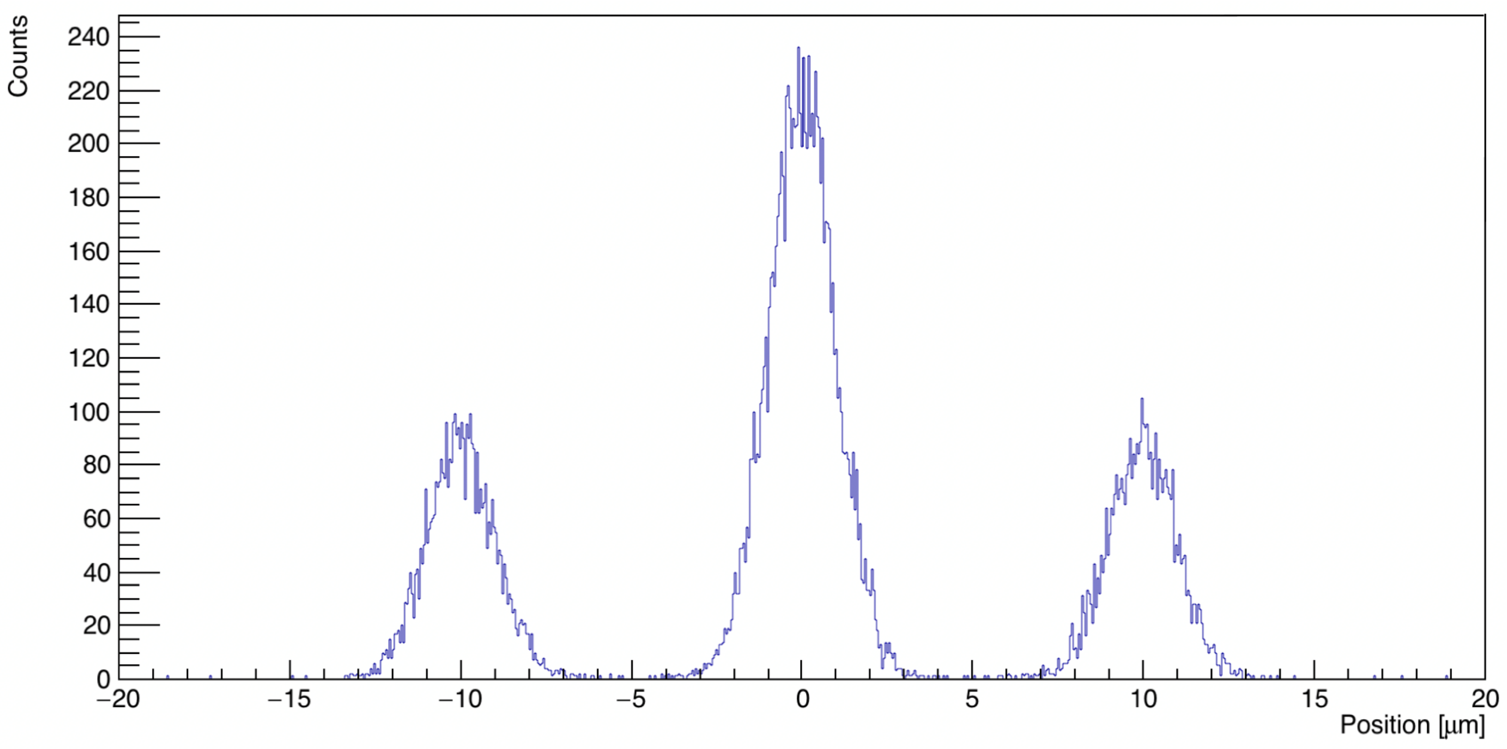
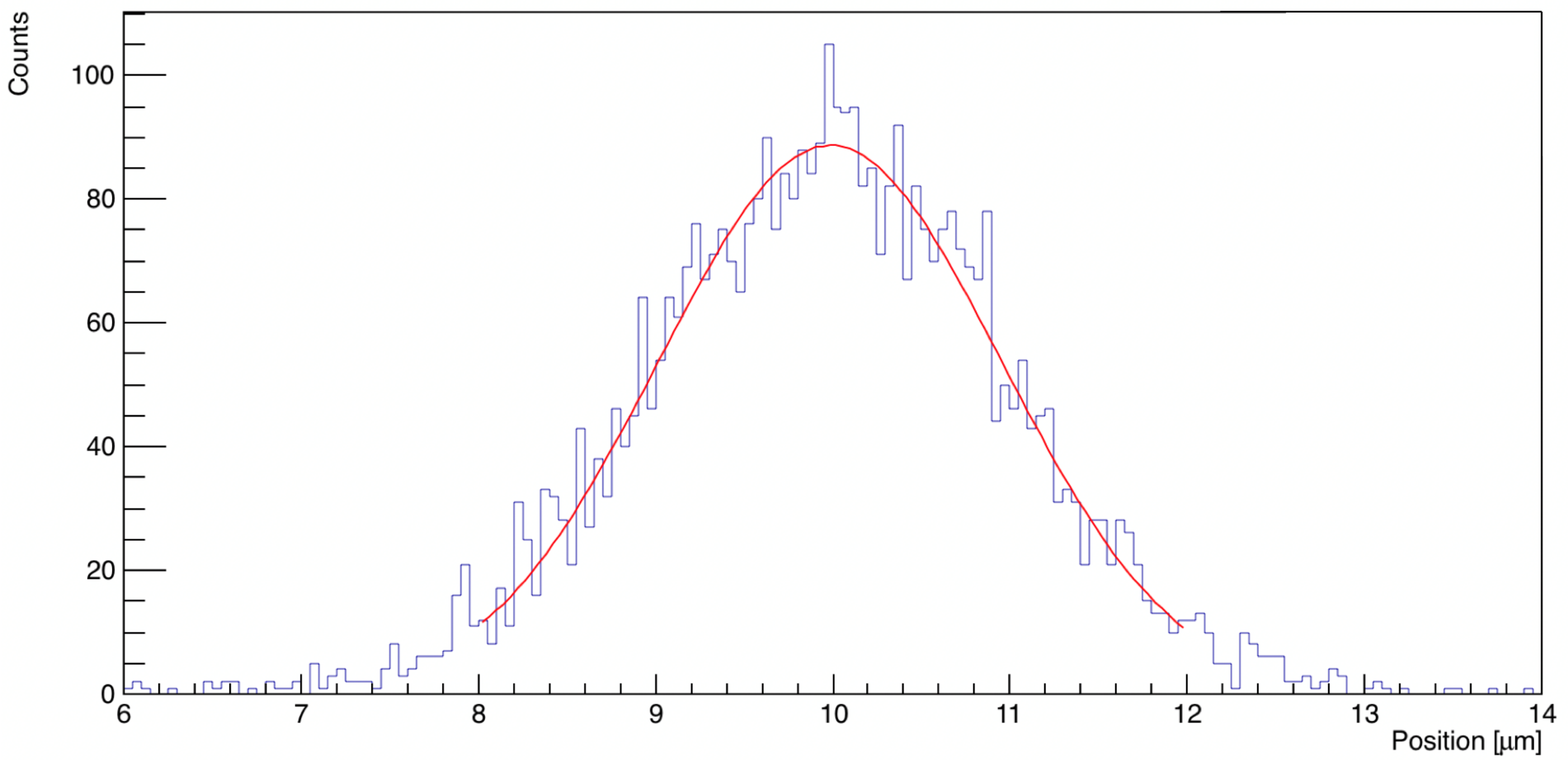
The Monte Carlo simulations confirm that for a given particle statistics the diffraction grating is preferable with respect to a few-slits system, as the interference peaks can be determined with a better resolution. The data reported in Figure 2 and Figure 3 refer to a distribution of particles of 10 keV kinetic energy on a screen located 1 m behind a diffraction grating having $N=100$ slits with $d=1.2$ μm and $a=d/2=0.6$ μm. One of the two first lateral interference peaks is fitted with a Gaussian distribution in an interval symmetric around the expected maximum position and for a counting level above approximately 10% of the maximum level. In the fitting procedure, the extrema of the interval are held fixed, whereas the central position and the spread of the Gaussian are free parameters. The error on the peak determination is defined as the absolute value of the difference between the theoretically expected maximum position and the central value of the Gaussian distribution obtained from the fit. Repeating the simulations for different numbers $N_r$ of random particles, and using several seeds for each $N_r$, it is found that an error on the determination of the maximum position systematically smaller than 50 nm is achieved with $N_r\ge \mathrm{20,000}$.

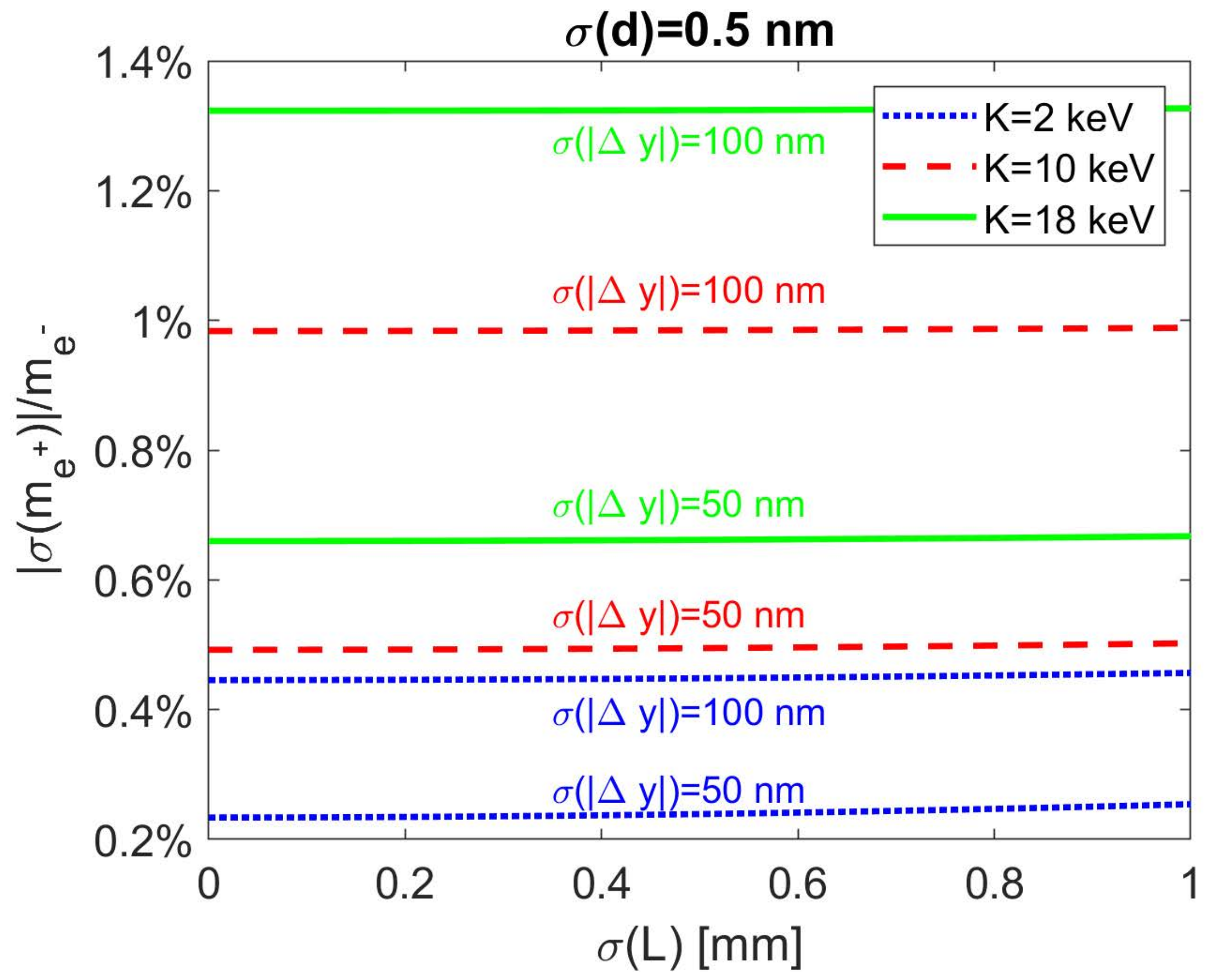
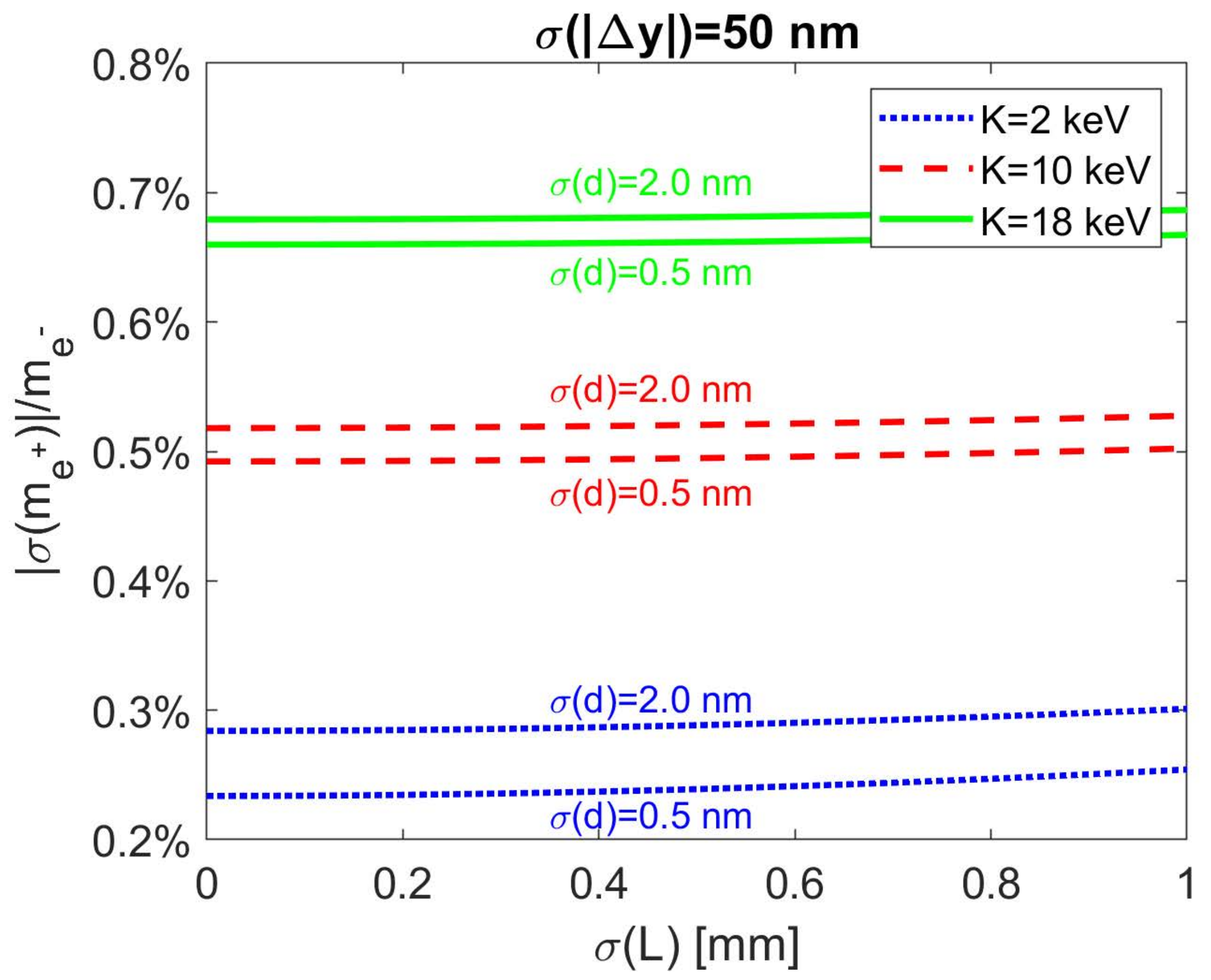
For a given detector, an example of error propagation analysis applied to the measurement of the positron mass based on Equation (8) is shown in Figure 4 and Figure 5. The error is normalized over the presently accepted value of the electron rest mass, $m_e$ [25]. The analysis refers to realistically attainable fixed values of the errors on d (see later) and $\mathsf{\Delta }y$ (intrinsic resolution of the emulsion detector). In this particular example, $L=1$ m, $d=1.2$ $\mathsf{\mu }$m, and the magnetic field strength is set to $B=0.01$ T, whereas the intensity of the electric field E is tuned to the particle velocity corresponding to K (for $m=m_e$). For K =10–20 keV, corresponding to the energy range of positrons in the QUPLAS-0 experiment [16], E would vary between approximately 500 and 1000 kV/m (for electrodes in the Wien filter spaced 10 mm apart, this corresponds to voltage differences of 5–10 kV between the electrodes; lower voltage differences can be considered with a smaller B field). The relative error on both E and B is assumed to be ${10}^{-3}$. Finally, for each K the value of $\left|\mathsf{\Delta }y\right|$ is set to the theoretical value (6) computed with the corresponding de Broglie wavelength (1) and assuming again $m=m_e$.

In general, the error on the mass increases with the particle kinetic energy. For a given interferometric setup (fixed L and d), the separation between the maxima of interference increases as the energy of the particles decreases (and therefore the de Broglie wavelength increases), so that these maxima are more clearly detectable. On the other hand, low energy particle are more strongly deviated by (transverse) residual magnetic fields present in the interferometer region (see discussion section), and the lower particle energy limit is eventually set by the sensitivity of the emulsion detector [22].

In addition, the error on the mass measurement turns out to be very weakly dependent on the relative errors on E ad B, while it is more strongly affected by the error on $\mathsf{\Delta }y$ (i.e., by the intrinsic resolution of the detector), as it is shown in Figure 4, in particular at higher kinetic energies, and by the error on the slit spacing d (see Figure 5). In the latter case, this error becomes more important at lower kinetic energies.

Keeping the same values of E and B in the Wien filter, the selected velocity is equal for particles (mass $m_1$) and antiparticles (mass $m_2$), and using the same interference apparatus (i.e., the same values of L and d), one finds for the ratio of the masses

$$\frac{m_2}{m_1}=\sqrt{\frac{1+{(L/\mathsf{\Delta }{y}_2)}^2}{1+{(L/\mathsf{\Delta }{y}_1)}^2}}\simeq \frac{|\mathsf{\Delta }{y}_1|}{|\mathsf{\Delta }{y}_2|},$$

(9)

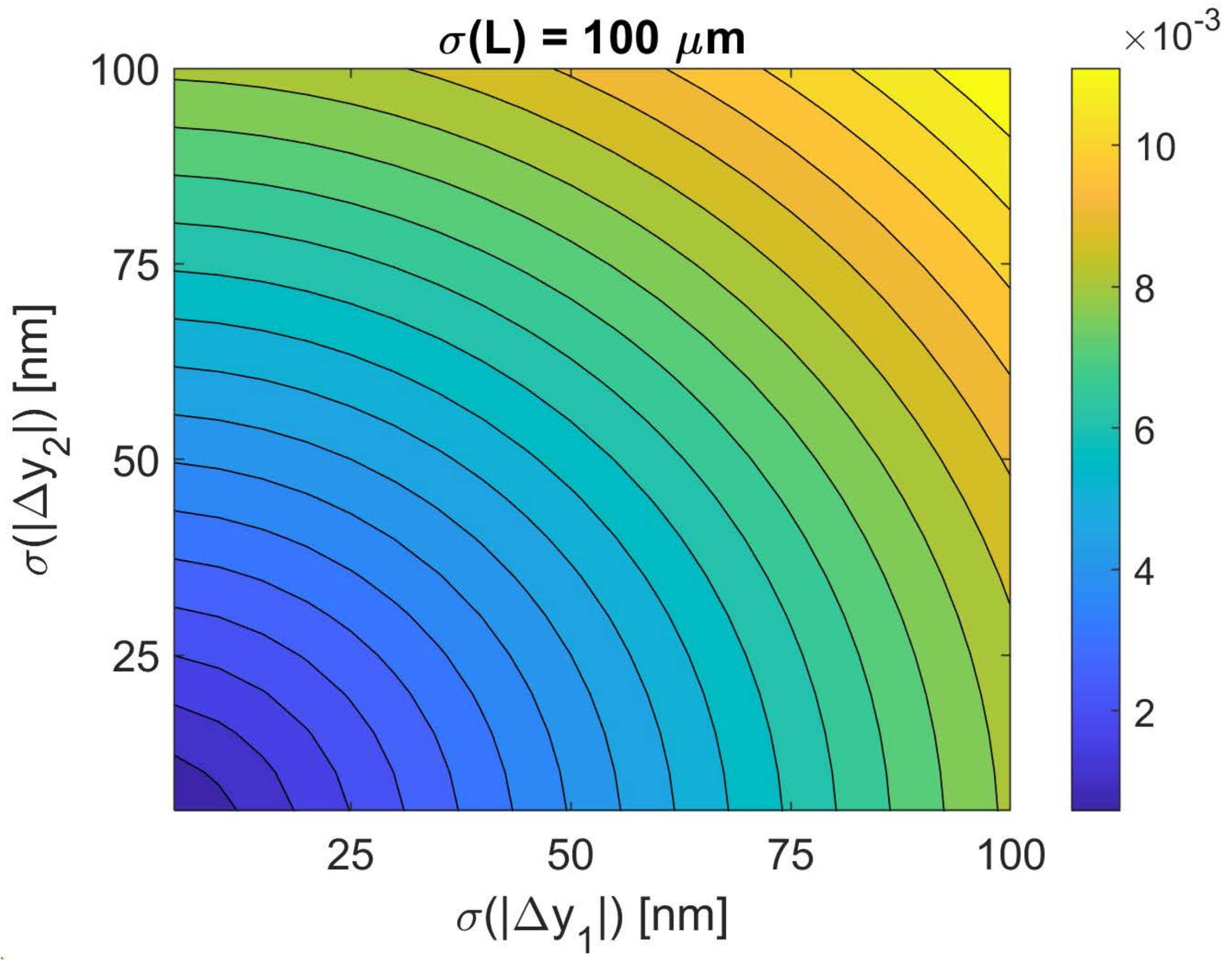
where $|\mathsf{\Delta }{y}_1|$ and $|\mathsf{\Delta }{y}_2|$ denote the distances between the first interference maxima for the particles of mass $m_1$ and $m_2$, respectively, and the simplification in the last formula follows from the approximation $L\gg |\mathsf{\Delta }{y}_{1,2}|$. In Equation (9), the effect of d, E, and B is eliminated. Some systematic errors tend therefore to cancel when the de Broglie wavelengths of a particle and of its antiparticle are measured in the same apparatus. An example of error propagation analysis on the mass ratio (9) between positron and electron is shown in Figure 6 (In the computations reported in Figure 4, Figure 5 and Figure 6 the values of the universal constants are $h=6.62607015\times {10}^{-34}$ Js (exact), c = 299,792,458 m/s (exact), $e=1.602176634\times {10}^{-19}$ C (exact) according to the 2019 revision of International System of Units [26], and the value $m_e=9.1093837015\left(28\right)\times {10}^{-31}$ kg (equivalent to $m_e{c}^2=510.99895000\left(15\right)$ keV) for the electron rest mass [25]). The results is computed for $\sigma \left(L\right)=100$ μm, but the effect on the results of the statistical error on L turns out to be completely negligible for reasonably small $\sigma \left(L\right)<1$ mm values.

When making the proposed measurement of the particle/antiparticle ratio, care must be taken to minimize any effect due to a different beam structure (divergence, spatial coherence) between the two types of particle. This can be achieved with a careful collimation that allows to coherently illuminate the spatial acceptance of the Wien filter.

3. Positrons and Electrons

The concept of measuring the de Broglie wavelength of particle and antiparticle in the same apparatus must be considered in light of the experimental constraints. For the case of electron and positron, the limiting factor is the statistics of the antiparticle beam.

Positron beams can be obtained in linear accelerators, at MeV energies or higher, or from radioactive sources such as ${}^{22}$Na. LINACs and high-energy facilities can offer high particles statistics [27], but the de Broglie wavelength of the particles is very small and the inherent bunching of particles makes them less suitable for use in interferometry setups. On the other hand, radioactive ${}^{22}$Na sources are employed that produce positrons by means of beta decays with a continuous distribution of kinetic energies up to 546 keV. These sources have an activity up to 50 mCi and the resulting positron spectra can be moderated to obtain a beam with well defined energy [28]. This process involves sizable particle losses so that the typical intensity of these continuous beams is of the order of ${10}^4$–${10}^5$ particles per second.

Interferometry can be profitably used under these conditions. In order to estimate reasonable values of the main involved parameters and their relevant accuracies, we refer here explicitly to the recent QUPLAS-0 experiment [15,16]. The kinetic energy of the positrons in this experiment (of the order of 10 keV) gives de Broglie wavelengths of the order of 10 pm, which are suitable for interferometric studies with material gratings.

QUPLAS-0 makes use of material diffraction gratings with micrometric periodicity [21,29]. The positron beam impinges on the gratings and forms an interferometric pattern on an emulsion detector [15,16]. A collimation stage improves the beam coherence and a germanium detector is used to monitor the particle flux by means of the 511 keV gammas generated by positron annihilations.

The uncertainties on K are determined by the initial kinetic energy distribution of the positrons after their moderation (≃1 eV), for instance, in an $\left[100\right]$-oriented tungsten single crystal foil with 1 $\mathsf{\mu }$m thickness, and by the uncertainty on the applied potentials (several keV) along the beamline, of the order of $0.1\%$. As discussed above, these uncertainties can be reduced with the use of suitable velocity selectors.

To estimate the uncertainty on the period d of the gratings used in the QUPLAS-0 experiment, we have to take into account that these gratings are extracted from a 100 mm diameter wafer [29]. The grating image recorded on the wafer is obtained by interfering two beams with spherical wavefronts. The image is therefore not uniform, with the grating period very slowly getting larger when moving away from the center of the wafer. To a very good approximation, the change in period $\mathsf{\Delta }d$ divided by the nominal period (the period at the center of the wafer) d is given by $\mathsf{\Delta }d/d\simeq r^2/2L^2$, where r is the distance from the center and L is the length of the interferometer arms, which is about 0.90 m in the used apparatus [29]. As a consequence, across each individual grating there is also a change in the period, but this error is about two orders of magnitude smaller than the error across a whole wafer.

The period of the “recorded” grating image was measured at the center of the exposure area, i.e., at the center of the wafer. The measured values are affected by random errors that are the result of an uncertainty in measuring angles (the rotation stage angle and the diffracted spot angle) [29]. Considering only those random errors, the measured periods for two different gratings were $d_1=1209.73\pm 0.29$ nm, and $d_2=1004.60\pm 0.28$ nm. Unfortunately, the location of the used gratings on the original wafer is unknown. By picturing a Gaussian spatial distribution of the gratings on the wafer with width $\sigma$ and with the wafer edge corresponding to 3 $\sigma$, and assuming our gratings most likely come from within a distance $r=25$ mm from the center (that is within approximately 1.5 $\sigma$), we can estimate $\mathsf{\Delta }d/d\simeq {25}^2/\left(2\right)\left({10}^6\right)\simeq 3.9\times {10}^{-4}$, which gives an error of $\mathsf{\Delta }d\simeq 0.39$ nm. Adding the two errors in quadrature, we obtain for the grating period $d_1=1209.73\pm 0.49$ nm and $d_2=1004.60\pm 0.48$ nm, respectively. Note that a comparably negligible contribution to the error comes also from the fact that the membranes may in principle distort due to temperature variations.

4. Discussion and Conclusions

In the previous analysis, we neglected all interactions of the interfering particles with the environment (e.g., van der Waals interactions). However, when transmitted by material gratings the particles are forced to pass at very short distances from the walls of the gratings (membranes with a slit width as small as 45 nm have been used in electron diffraction experiments [30]). This inevitably results in an interaction mediated by a potential [31]. Such issues might be avoided with the use of light gratings [32].

It has also been implicitly assumed that the contrast is sufficiently high so that the periodicity of the pattern on the position-sensitive detector is clearly visible. Effects which may degrade the contrast are related to the misalignments of the optical elements, and the presence of external fields and/or beam–beam interactions. In particular, while working with charged particles a field-free environment is crucial for avoiding decoherence effects and pattern distortions within the interferometer. As indicated in Figure 1, the interferometer can be placed inside a cylindrical mu-metal shield to reduce the effects of magnetic fields. Mu-metal is a nickel-iron soft ferromagnetic alloy with very high permeability, that leads to the concentration of the magnetic flux into the material, resulting in a lower field inside the tube. Typical shielding factors can reach 1000 or more. In any case, it has to be underlined that a global shift (linearly dependent on the strength of the residual magnetic field, and on opposite sides for particles and antiparticles) of the diffraction pattern will be unavoidably present due to the Earth’s magnetic field. This can be sizable especially at low kinetic energies: approximately 5 to 20 $\mathsf{\mu }$m for K from 20 to 1 keV, assuming a constant Earth’s magnetic field of 0.5 Gauss transverse to the beam and a uniform shielding factor of 1000. What could possibly affect the measurement are time fluctuations of the ambient magnetic field, but assuming a relative variation of the magnetic field strength not greater that ${10}^{-3}$ and again a shielding factor of 1000, particle deviations of approximately 5 to 20 nm are expected for K from 20 to 1 keV, i.e., smaller than the emulsion resolution.

In the configuration presented in Figure 1, we have assumed that the only forces acting on the particle are the E and B fields in the Wien filter. Gravitation is of course present, but the overall vertical deflection over a distance L of the order of 1 m is completely negligible (much less than 1 nm) for particles (electrons or protons) with keV energies. In principle, gravitation might play a role if there is a different response between particles and antiparticles to the Earth gravitational field in the Wien filter, since with a suitable rotation of the apparatus this may lead to slightly different velocities (and therefore de Broglie wavelengths) at the exit of the filter, but again this effect turns out to be negligibly small, and masked by the uncertainties in all relevant quantities entering Equation (8).

In conclusion, it has been shown that interferometric methods can be used to obtain a direct estimate of particle/antiparticle masses. In particular, some systematics cancels out is the particle and the antiparticle mass are measured through the de Broglie wavelength in the same apparatus.

The method proposed here can be applied to any charged particle for its absolute mass measurement as well as to any particle–antiparticle pair for the measurement of their mass ratio. This, however, typically requires adjusting the interferometric parameters to the case under consideration.

For example, for the case of hadronic systems, like protons and antiprotons, one can note that spectroscopy has been used to estimate the proton-to-antiproton charge-to-mass ratio with a precision of 69 parts per trillion [14]. In this regard, an interferometric measurement would instead depend only on the masses without having to rely on the equality of the charges.

This approach is made possible thanks to the availability of low-energy antiprotons at the new ELENA facility of the CERN Antiproton Decelerator [33,34]. For instance, the ASACUSA experiment [35] is planning to extract a low-energy antiproton beam from its MUSASHI trap or from the planned Reservoir under construction [36]. Energies at the level of 10 eV can be obtained and the availability of protons and antiprotons in the same beam source makes possible interferometric experiments with a de Broglie wavelength of 10 pm. This wavelength is about the same that was used (for positrons) in the QUPLAS-0 experiment. As the same beamline can accommodate both protons and antiprotons, an interferometric experiment can be performed along the lines outlined here.

References

- Sturm, S.; Köhler, F.; Zatorski, J.; Wagner, A.; Harman, Z.; Werth, G.; Quint, W.; Keitel, C.H.; Blaum, K. High-precision measurement of the atomic mass of the electron. Nature 2014, 506, 467. [Google Scholar] [CrossRef]
- Köhler, F.; Sturm, S.; Kracke, A.; Werth, G.; Quint, W.; Blaum, K. The electron mass from g-factor measurements on hydrogen-like carbon 12C5+. J. Phys. B At. Mol. Opt. Phys. 2015, 48, 144032. [Google Scholar] [CrossRef] [Green Version]
- Heiße, F.; Köhler-Langes, F.; Rau, S.; Hou, J.; Junck, S.; Kracke, A.; Mooser, A.; Quint, W.; Ulmer, S.; Werth, G.; et al. High-Precision Measurement of the Proton’s Atomic Mass. Phys. Rev. Lett. 2017, 119, 033001. [Google Scholar] [CrossRef] [Green Version]
- Hori, M.; Aghai-Khozani, H.; Sótér, A.; Barna, D.; Dax, A.; Hayano, R.; Kobayashi, T.; Murakami, Y.; Todoroki, K.; Yamada, H.; et al. Buffer-gas cooling of antiprotonic helium to 1.5 to 1.7 K, and antiproton-to-electron mass ratio. Science 2016, 354, 610. [Google Scholar] [CrossRef]
- Lehnert, R. CPT Symmetry and Its Violation. Symmetry 2016, 8, 214. [Google Scholar] [CrossRef] [Green Version]
- Lüders, G. Proof of the TCP theorem. Ann. Phys. 1957, 2, 1. [Google Scholar] [CrossRef]
- Greenberg, O.W. CPT Violation Implies Violation of Lorentz Invariance. Phys. Rev. Lett. 2002, 89, 231602. [Google Scholar] [CrossRef] [PubMed] [Green Version]
- Kostelecký, V.A.; Samuel, S. Spontaneous breaking of Lorentz symmetry in string theory. Phys. Rev. D 1989, 39, 683. [Google Scholar] [CrossRef] [Green Version]
- Fee, M.S.; Chu, S.; Mills, A.P., Jr.; Chichester, R.J.; Zuckerman, D.M.; Shaw, E.D.; Danzmann, K. Measurement of the positronium 1 3S1–2 3S1 interval by continuous-wave two-photon excitation. Phys. Rev. A 1993, 48, 192. [Google Scholar] [CrossRef] [Green Version]
- Dolgov, A.D.; Novikov, V.A. A cosmological bound on e+-e- mass difference. Phys. Lett. B 2014, 732, 244. [Google Scholar] [CrossRef] [Green Version]
- Zyla, P.A.; Barnett, R.M.; Beringer, J.; Dahl, O.; Dwyer, D.A.; Groom, D.E.; Lin, C.-J.; Lugovsky, K.S.; Pomarol, A.; Particle Data Group; et al. Review of Particle Physics. Prog. Theor. Exp. Phys. 2020, 2020, 083C01. [Google Scholar] [CrossRef]
- Hori, M.; Sótér, A.; Barna, D.; Dax, A.; Hayano, R.; Friedreich, S.; Juhász, B.; Pask, T.; Widmann, E.; Horváth, D.; et al. Two-photon laser spectroscopy of antiprotonic helium and the antiproton-to-electron mass ratio. Nature 2011, 475, 484. [Google Scholar] [CrossRef] [Green Version]
- Gabrielse, G.; Khabbaz, A.; Hall, D.S.; Heimann, C.; Kalinowsky, H.; Jhe, W. Precision Mass Spectroscopy of the Antiproton and Proton Using Simultaneously Trapped Particles. Phys. Rev. Lett. 1999, 82, 3198. [Google Scholar] [CrossRef] [Green Version]
- Ulmer, S.; Smorra, C.; Mooser, A.; Franke, K.; Nagahama, H.; Schneider, G.; Higuchi, T.; Van Gorp, S.; Blaum, K.; Matsuda, Y.; et al. High-precision comparison of the antiproton-to-proton charge-to-mass ratio. Nature 2015, 524, 196. [Google Scholar] [CrossRef] [Green Version]
- Sala, S.; Ariga, A.; Ereditato, A.; Ferragut, R.; Giammarchi, M.; Leone, M.; Pistillo, C.; Scampoli, P. First demonstration of antimatter wave interferometry. Sci. Adv. 2019, 5, eaav7610. [Google Scholar] [CrossRef] [Green Version]
- Ariga, A.; Cialdi, S.; Costantini, G.; Ereditato, A.; Ferragut, R.; Giammarchi, G.; Leone, M.; Maero, G.; Miramonti, L.; Pistillo, C.; et al. The QUPLAS experimental apparatus for antimatter interferometry. Nucl. Instrum. Meth. Phys. Res. A 2020, 951, 163019. [Google Scholar] [CrossRef]
- De Broglie, L. Recherches sur la théorie des Quanta. Ann. Phys. 1925, 10, 22. [Google Scholar] [CrossRef] [Green Version]
- Rose, H.H. Optics of high-performance electron microscopes. Sci. Technol. Adv. Mater. 2008, 9, 014107. [Google Scholar] [CrossRef] [PubMed]
- Plies, E.; Marianowski, K.; Ohnweiler, T. The Wien filter: History, fundamentals and modern applications. Nucl. Instrum. Meth. Phys. Res. A 2011, 645, 7. [Google Scholar] [CrossRef]
- Aghion, S.; Ariga, A.; Ariga, T.; Bollani, M.; Dei Cas, E.; Ereditato, A.; Evans, C.; Ferragut, R.; Giammarchi, M.; Pistillo, C.; et al. Detection of low energy antimatter with emulsions. J. Instrum. 2016, 11, P06017. [Google Scholar] [CrossRef] [Green Version]
- Aghion, S.; Ariga, A.; Bollani, M.; Ereditato, A.; Ferragut, R.; Giammarchi, M.; Lodari, M.; Pistillo, C.; Sala, S.; Scampoli, P.; et al. Nuclear emulsions for the detection of micrometric-scale fringe patterns: An application to positron interferometry. J. Instrum. 2018, 13, P05013. [Google Scholar] [CrossRef] [Green Version]
- Anzi, L.; Ariga, A.; Ereditato, A.; Ferragut, R.; Giammarchi, M.; Maero, G.; Pistillo, C.; Romé, M.; Scampoli, P.; Toso, V. Sensitivity of emulsion detectors to low energy positrons. J. Instrum. 2020, 15, 03027. [Google Scholar] [CrossRef]
- Asada, T.; Naka, T.; Kuwabara, K.; Yoshimoto, M. The development of a super-fine-grained nuclear emulsion. Prog. Theor. Exp. Phys. 2017, 2017, 063H01. [Google Scholar] [CrossRef] [Green Version]
- Alexandrov, A.; Asada, T.; De Lellis, G.; Di Crescenzo, A.; Gentile, V.; Naka, T.; Tioukov, V.; Umemoto, A. Super-resolution high-speed optical microscopy for fully automated readout of metallic nanoparticles and nanostructures. Sci. Rep. 2020, 10, 18773. [Google Scholar] [CrossRef]
- Fundamental Physical Constants. Available online: https://physics.nist.gov/cgi-bin/cuu/Value?me (accessed on 5 June 2021).
- The International System of Units. Available online: https://www.bipm.org/utils/common/pdf/si-brochure/SI-Brochure-9.pdf (accessed on 5 June 2021).
- Hugenschmidt, C. Positrons in surface physics. Surf. Sci. Rep. 2016, 71, 547. [Google Scholar] [CrossRef] [Green Version]
- Coleman, P. Positron Beams and Their Applications; World Scientific: Singapore, 2000. [Google Scholar] [CrossRef]
- Maskless Photolithography & Nanofabrication Services. Available online: https://www.lumarray.com/ (accessed on 5 June 2021).
- McMorran, B.; Perreault, J.D.; Savas, T.A.; Cronin, A. Diffraction of 0.5 keV electrons from free-standing transmission gratings. Ultramicroscopy 2006, 106, 356. [Google Scholar] [CrossRef] [PubMed] [Green Version]
- Sala, S.; Castelli, F.; Giammarchi, M.; Siccardi, S.; Olivares, S. Matter-wave interferometry: Towards antimatter interferometers. J. Phys. B 2015, 48, 195002. [Google Scholar] [CrossRef] [Green Version]
- Cronin, A.D.; Schmiedmayer, J.; Pritchard, D.E. Optics and interferometry with atoms and molecules. Rev. Mod. Phys. 2009, 81, 1051. [Google Scholar] [CrossRef]
- Maury, S.; Oelert, W.; Bartmann, W.; Belochitskii, P.; Breuker, H.; Butin, F.; Carli, C.; Eriksson, T.; Pasinelli, S.; Tranquille, G. ELENA: The extra low energy anti-proton facility at CERN. Hyperfine Interact. 2014, 229, 105. [Google Scholar] [CrossRef]
- Bartmann, W.; Belochitskii, P.; Breuker, H.; Butin, F.; Carli, C.; Eriksson, T.; Oelert, W.; Ostojic, R.; Pasinelli, S.; ELENA and AD teams Gerard Tranquille. The ELENA facility. Philos. Trans. R. Soc. A 2018, 376, 20170266. [Google Scholar] [CrossRef]
- Kuroda, N.; Ulmer, S.; Murtagh, D.J.; Gorp, S.V.; Nagata, Y.; Diermaier, M.; Federmann, S.; Leali, M.; Malbrunot, C.; Mascagna, V.; et al. A source of antihydrogen for in-flight hyperfine spectroscopy. Nat. Commun. 2014, 5, 3089. [Google Scholar] [CrossRef] [Green Version]
- Hori, M.; Widmann, E. Asacusa Proposal for Elena. CERN Report SPSC-P-307-ADD-2. 2019. Available online: https://cds.cern.ch/record/2691506/files/SPSC-P-307-ADD-2.pdf (accessed on 5 June 2021).
Figure 1.
Scheme of the proposed apparatus. After an acceleration stage, the charged particles enter a Wien filter. Particles with velocity v equal to the ratio between the electric and the magnetic field pass through the filter without undergoing deflection and impinge on an optical grating. An interferometric pattern is formed on an a position-sensitive screen (emulsion detector) located at a distance L from the grating. The interferometer is placed inside a cylindrical mu-metal shield to reduce the effects of external magnetic fields (e.g., the Earth’s magnetic field).
Figure 2.
Histogram of 20,000 particles randomly generated according to the theoretical distribution Equation (4).
Figure 3.
Fit of one of the first lateral interference peaks shown in Figure 2 with a Gaussian distribution.
Figure 4.
Error on the positron mass, , normalized over the electron rest mass, [25], vs the error on the distance L between the two gratings, for three different values of the kinetic energy K. For each K value the lower and upper curves, refer to nm and nm, respectively; nm in all cases.
Figure 5.
The same as in Figure 4. For each K value the lower and upper curves refer to nm and nm, respectively; nm in all cases.
Figure 6.
Error on the positron to electron mass ratio vs the statistical errors on and .
Publisher’s Note: MDPI stays neutral with regard to jurisdictional claims in published maps and institutional affiliations. |
© 2021 by the authors. Licensee MDPI, Basel, Switzerland. This article is an open access article distributed under the terms and conditions of the Creative Commons Attribution (CC BY) license (https://creativecommons.org/licenses/by/4.0/).
Share and Cite
MDPI and ACS Style
Pasino, E.; Cialdi, S.; Costantini, G.; Ferragut, R.; Giammarchi, M.; Migliorati, S.; Romé, M.; Savas, T.; Toso, V. An Interferometric Method for Particle Mass Measurements. Symmetry 2021, 13, 1232. https://doi.org/10.3390/sym13071232
AMA Style
Pasino E, Cialdi S, Costantini G, Ferragut R, Giammarchi M, Migliorati S, Romé M, Savas T, Toso V. An Interferometric Method for Particle Mass Measurements. Symmetry. 2021; 13(7):1232. https://doi.org/10.3390/sym13071232
Chicago/Turabian StylePasino, Eleonora, Simone Cialdi, Giovanni Costantini, Rafael Ferragut, Marco Giammarchi, Stefano Migliorati, Massimiliano Romé, Timothy Savas, and Valerio Toso. 2021. "An Interferometric Method for Particle Mass Measurements" Symmetry 13, no. 7: 1232. https://doi.org/10.3390/sym13071232
Note that from the first issue of 2016, this journal uses article numbers instead of page numbers. See further details here.