A Filter and Nonmonotone Adaptive Trust Region Line Search Method for Unconstrained Optimization


1
School of Science, Southwest Petroleum University, Chengdu 610500, China
2
School of Artificial Intelligence, Southwest Petroleum University, Chengdu 610500, China
*
Author to whom correspondence should be addressed.
Symmetry 2020, 12(4), 656; https://doi.org/10.3390/sym12040656
Submission received: 20 March 2020
/
Revised: 1 April 2020
/
Accepted: 3 April 2020
/
Published: 21 April 2020
(This article belongs to the Special Issue Advance in Nonlinear Analysis and Optimization)
Abstract
:In this paper, a new nonmonotone adaptive trust region algorithm is proposed for unconstrained optimization by combining a multidimensional filter and the Goldstein-type line search technique. A modified trust region ratio is presented which results in more reasonable consistency between the accurate model and the approximate model. When a trial step is rejected, we use a multidimensional filter to increase the likelihood that the trial step is accepted. If the trial step is still not successful with the filter, a nonmonotone Goldstein-type line search is used in the direction of the rejected trial step. The approximation of the Hessian matrix is updated by the modified Quasi-Newton formula (CBFGS). Under appropriate conditions, the proposed algorithm is globally convergent and superlinearly convergent. The new algorithm shows better performance in terms of the Dolan–Moré performance profile. Numerical results demonstrate the efficiency and robustness of the proposed algorithm for solving unconstrained optimization problems.
1. Introduction
Consider the following unconstrained optimization problem:
where : is a twice continuously differentiable function. The problem has widely used in many applications based on medical science, optimal control, and functional approximation, etc. As we all know, there are many methods for solving unconstrained optimization problems, such as the conjugate gradient method [1,2,3], the Newton method [4,5], and the trust region method [6,7,8]. Constrained optimization problems can also be solved by processing constraint conditions and transforming them into unconstrained optimization problems. Motivated by this, it is quite necessary to propose a new modified trust region method for solving unconstrained optimization problems.
As is commonly known, the trust region method and the line search method are two frequently used iterative methods. Line search methods involve the process of calculating the step length in the specific direction and driving a new point as . The primary idea of the trust region method is as follows: at current iteration point , the trial step is obtained by solving the following subproblem:
where is the Euclidean norm, , , is a symmetric approximation matrix of , and is a trust region radius.
Traditional trust region methods have some disadvantages, such as the fact that the subproblem needs to be solved many times to obtain an acceptable trial step within one iteration, which leads to high computational costs for the iterative process. One way to overcome this disadvantage is to use a line search strategy in the direction of the rejected trial step. Based on this situation, Nocedal and Yuan [9] proposed an algorithm in 1998, combining the trust region method and the line search method for the first time. Inspired by this, Michael et al., Li et al., and Zhang et al. proposed a trust region method with the line search strategy ([10,11,12], respectively).
As can be seen in other works [4,7,8] monotone techniques are distinguished from nonmonotone techniques in that the value of the function needs to be reduced at each iteration; at the same time, the use of nonmonotone techniques can not only guarantee finding the global optimal solution effectively, but also improve the convergence rate of the algorithm. The watchdog technique was presented by Chamberlain et al. [13] in 1982 to overcome the Maratos effect of constrained optimization problems. Motivated by this idea, a nonmonotone line search technique was proposed by Grippo et al. [14] in 1986. The step length satisfies the following inequality:
where ,, , , and is an integer constant.
However, the common nonmonotone term suffers from various drawbacks. For example, the valid value of the produced function in any iteration is essentially discarded, and the numerical results highly depend on the choice of . To overcome these drawbacks, Cui et al. [15] proposed another nonmonotone line search method as follows:
where the nonmonotone term is defined by
and
where , , , and .
Based on this idea, in order to include the minimum value of in an acceptable interval and keep the consistency of the nonmonotone term, we proposed a trust region method with the Goldstein-type line search technique. The step length satisfies the following inequalities:
where
, , , , and .
To evaluate the consistency between the quadratic model and the objective function, the ratio is defined by Ahookhosh et al. [16] as follows:
It is well-known that the adaptive radius plays a valuable role in performance. In 1997, an adaptive strategy for automatically determining the initial trust region radius was proposed by Sartenear [17]. However, it can be seen that the gradient or Hessian information is not explicitly used to update the radius. Motivated by the first-order information and second-order information of the objective function, Zhang et al. [18] proposed a new scheme to determine trust region radius in 2002 as follows: , where ,. In order to avoid computing the inverse of the matrix and the Euclidean norm of at each iteration point , Zhou et al. [19] proposed an adaptive trust region radius as follows: , where , and and are parameters. Prompted by the adaptive technique, Wang et al. [8] proposed a new adaptive trust region radius as follows: , which reduces the related workload and calculation time. Based on this fact, other authors also proposed modified adaptive trust region methods [20,21,22].
In order to overcome the difficulty of selecting penalty factors when using penalty functions, Fletcher et al. first recommended the filter techniques for constrained nonlinear optimization (see [23] for details). More recently, Gould et al. [24] explored a new nonmonotone trust region method with multidimensional filter techniques for solving unconstrained optimization problems. This idea incorporates the concept of nonmonotone to build a filter that can reject poor iteration points, and enforce convergence from random starting points. At the same time, the prototype of the multidimensional filter techniques relax the requirements of monotonicity in the classic trust region framework. This idea has been popularized by some authors [25,26,27].
In the following, we refer to by ; when the component of is needed, it is denoted with , where . We say that an iteration point dominates whenever
where is a small positive constant.
Based on [8], we know that a multidimensional filter is a list of -tuples of the form , such that
where and belong to .
For all , a new trial point is acceptable if there exists , such that
where and are positive constants, and and satisfy the inequality .
When an iteration point is accepted by the filter, we add to the filter, and with the following property
is removed from the filter.
The rest of this article is organized as follows. In Section 2, we describe a new nonmonotone adaptive trust region algorithm. We establish the global convergence and superlinear convergence of the algorithm in Section 3. In Section 4, numerical results are given, which show that the new method is effective. Finally, some concluding comments are provided in Section 5.
2. The new algorithm
In this section, a new filter and nonmonotone adaptive trust region Goldstein-type line search method is proposed. The trust region ratio is used to determine whether the trial step is accepted. Following the trust region ratio of Ahookhosh et al. in [16], we define a modified form as follows:
We can see that the effect of nonmonotonicity can be controlled the numerator and denominator, respectively. Thus, the new trust region ratio may find the global optimal solution effectively. Compared with the general filter trust region algorithm in [24], we propose a new criteria, that is, whether the trial point satisfies , and verify whether it is accepted by the filter .
At the same time, a new adaptive trust region radius is presented as follows:
where , , and is a nonnegative integer. Compared with the adaptive trust region method in [8], the new method has the following effective properties: the parameter plays a vital role in adjusting the radius, and it can also reduce the workload and computational time. However, the new trust region radius only uses gradient function information, not function information.
On the other hand, in each iteration, is the trial step to be calculated by
More formally, a filter and nonmonotone adaptive trust region line search method, which we call the FNATR, is described as follows.
| Algorithm 1. A new filter and nonmonotone adaptive trust region line search method. |
| Step 0. (Initialization) Start with and the symmetric matrix . The constants , , , , , and are also given. Set , . |
| Step 1. If , then stop. |
| Step 2. Solve the subproblems of Equations (18) and (19) to find the trial step , set . |
| Step 3. Compute and , respectively. |
| Step 4. Test the trial step. |
| If , then set , , and go to Step 5. |
| Otherwise, compute . |
| if is accepted by the filter , then ; add into the filter , and go to Step 5. |
| Otherwise, find the step length , satisfying Equations (8) and (9), and set . Then, set |
| , and go to Step 5. |
| Step 5. Update the symmetric matrix by using a modified Quasi-Newton formula. Set , , and go to Step 1. |
In particular, we consider the following assumptions to analyze the convergence properties of Algorithm 1.
Assumption 1.
The level setsatisfies;is continuously differentiable and has a lower bound.
Assumption 2.
The matrixis uniformly bounded, i.e., there exists a constantsuch that.
Remark 1.
There is a constant;is a positive definite symmetric matrix, andsatisfies the following inequalities:
Remark 2.
Ifis continuously differentiable andis Lipschitz continuous, there is a positive constantso that
3. Convergence Analysis
In order to easily derive convergence results, we define the following indexes: , , and . Then, . At the time of , we obtain .
Lemma 1.
Suppose that Assumptions 1 and 2 holds, andis the solution of Equation (18); then,
Proof.
According to , we have . Thus, we obtain
Taking into account Equation (24) and Remark 1, we can conclude that Equation (23) holds. □
Lemma 2.
For all, we can find that
Proof.
The proof can be obtained by Taylor’s expansion and H3. □
Lemma 3.
Suppose that the infinite sequence is generated by Algorithm 1. The number of successful iterations is infinite, that is,. Then, we have.
Proof.
We can proceed by induction. When , apparently we obtain .
Assuming that holds, we get . Then, we prove . Consider the following two cases:
Case 1: When , according to Equation (16) we have,
Thus,
According to Equations (23) and (27), we can obtain . Using the definition of and , we get
The above two inequalities show that
Case 2: When , according to , we have . Thus, we obtain . This shows the sequence . □
Lemma 4.
Suppose that Assumptions 1 and 2 holds, and the sequenceis generated by Algorithm 1. Then, the sequenceis not monotonically increasing and convergent.
Proof.
The proof is similar to the proof of Lemma 5 in [8] and is here omitted. □
Lemma 5.
Suppose that Assumptions 1 and 2 holds, and the sequenceis generated by Algorithm 1. Moreover, assume that there exists a constant, so that, for all. Then, Algorithm 1 is well defined; that is, the algorithm terminates in a limited number of steps.
Proof.
In contradiction, suppose that Algorithm 1 cycles infinitely at iteration . Then, we have
Following Equation (17), we have as . Thus, we get,
where is a solution of the subproblem of Equation (18) corresponding to in the iteration. Combining Lemma 1, Lemma 2, and Equation (28), we obtain
which implies that there exists a sufficiently large such that as . This contradicts Equation (30), and shows that Algorithm 1 is well defined. □
Lemma 6.
Suppose that Assumptions 1 and 2 holds, and there exists a constantsuch thatfor all. Therefore, there is a constantsuch that
Proof.
The proof is similar to that of Theorem 6.4.3 in [28], and is therefore omitted here. □
In what follows, we establish global convergence of Algorithm 1 based on the above and the lemmas.
Theorem 1.
(Global Convergence) Suppose that Assumptions 1 and 2 holds, and the sequenceis generated by Algorithm 1, such that,
Proof.
Divide the proof into the following two cases:
Case 1: The number of successful iterations and many filter iterations are infinite, i.e., , .
Suppose, on the contrary, that Equation (34) does not hold. Thus, there exists a constant such that , as is sufficiently large. Introduce the index of set . Following Assumption 1, we can find that is bounded. Therefore, there is a subsequence such that
where is a constant. The iteration point is accepted by the filter ; then there exists , for every , that is
As is sufficiently large, we have
However, we obtain , which means that Equation (37) does not hold. The proof is completed.
Case 2: The number of successful iterations is infinite, and the number of filter iterations is finite, i.e., , .
We proceed from the following proof with a contradiction. Suppose that there exists a constant , such that , for sufficiently large . Based on , for sufficiently large , we have . Thus, set
Based on Assumption 2, Equation (28), Lemma 1, and Lemma 6, we write
As and are sufficiently large, according to and , we know that is sufficiently large. Thus, we can find that , and the left end of Equation (39) has no lower bound. We can deduce that
Using Lemma 4, as and are sufficiently large, the left end of Equation (40) has a lower bound, which contradicts Equation (39). This completes the proof of Theorem 1. □
Now, based on the appropriate conditions, the following superlinear convergence is presented for Algorithm 1.
Theorem 2.
(Superlinear Convergence) Suppose that Assumptions 1 and 2 holds, and the sequencegenerated by Algorithm 1 converges to. Moreover, it is reasonable to assume that the Hessian matrixis positive definite. If, where, and
then the sequenceconverges toin a superlinear manner.
Proof.
Found using the same method as in the proof of Theorem 4.1 in [29]. □
4. Preliminary Numerical Experiments
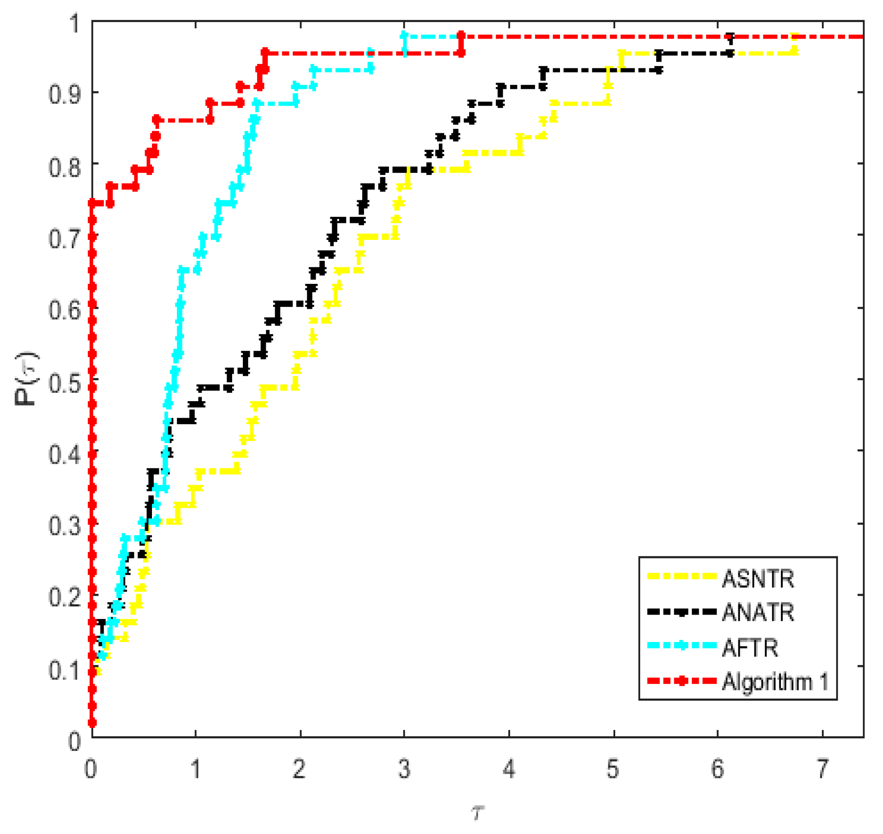
In this section, we present numerical results to illustrate the performance of Algorithm 1 in comparison with the standard nonmonotone trust region algorithm of Pang et al. in [30] (ASNTR), the nonmonotone adaptive trust region algorithm of Ahookhoosh et al. in [16] (ANATR), and the multidimensional filter trust region algorithm of Wang et al. in [8] (AFTR). We performed our codes in double precision format of algorithm in MATLAB 9.4 programming, and the codes are given in the Appendix A. A set of unconstrained optimization test problems are selected from Andrei [31] with the some medium-scale and large-scale problems. The stopping criteria are that the number of iterations exceeds 10,000 or . ,, and CPU represent the total number of function evaluations, the total number of gradient evaluations, and running time in seconds, respectively. Following Step 0, we exploit the following values:, , , , , , , , and . In addition, is updated by the following recursive formula:
The matrix is updated using a CBFGS formula [32]:
where , and .
In Table 1, it is easily can be seen that Algorithm 1 outperforms the ASNTR, ANATR, and AFTR algorithms with respect to , , and CPU, especially for some problems. The Dolan–Moré [33] performance profile was used to compare the efficiency using the number of functional evaluations, the number of gradient evaluations, and running time. A performance index can be selected as measure of comparison among the mentioned algorithms, and the results can be illustrated by a performance profile. For every , the performance profile gives the proportion of the test problems. The performance of each considered algorithmic variant was the best within a range of of the best.
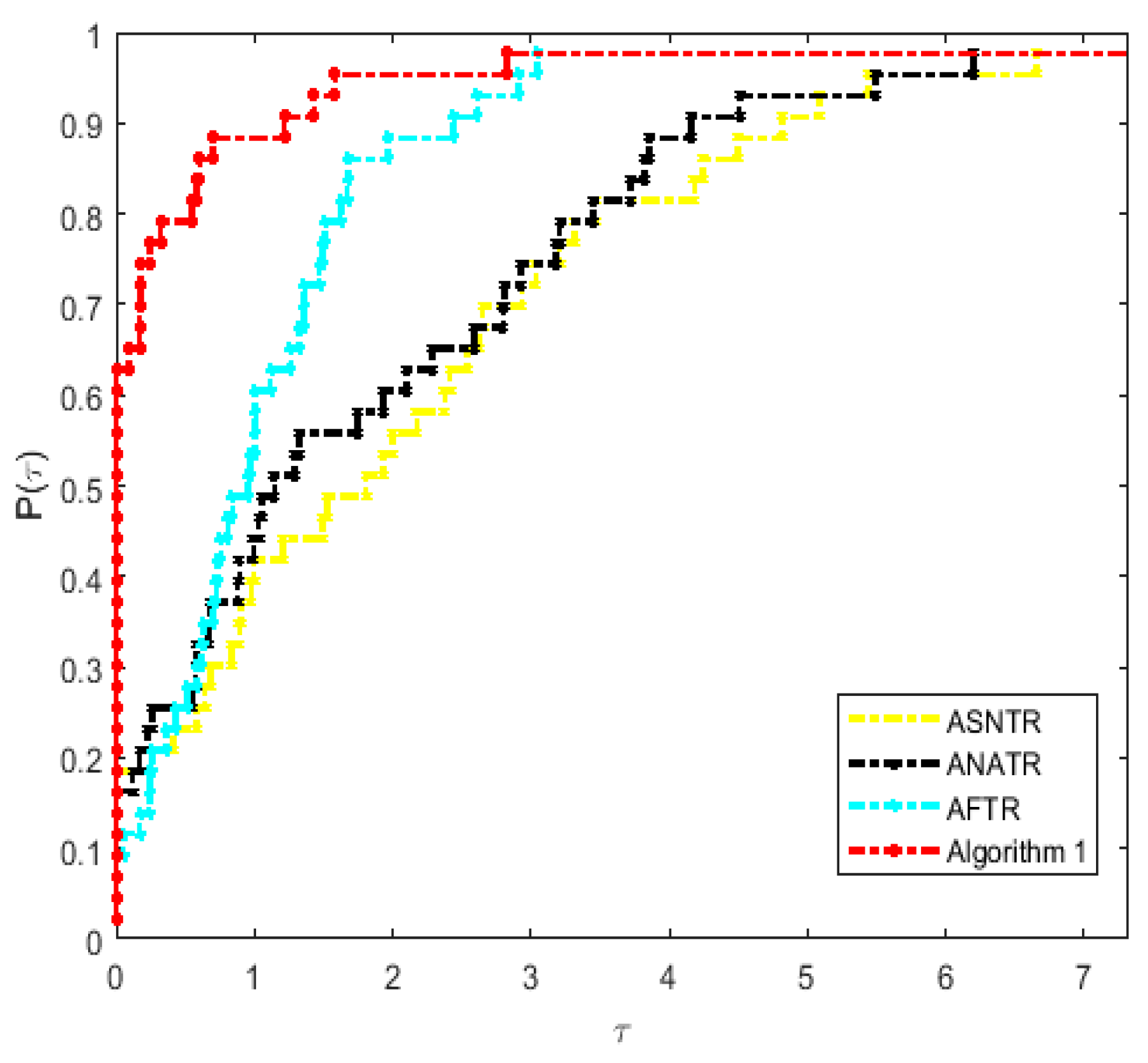
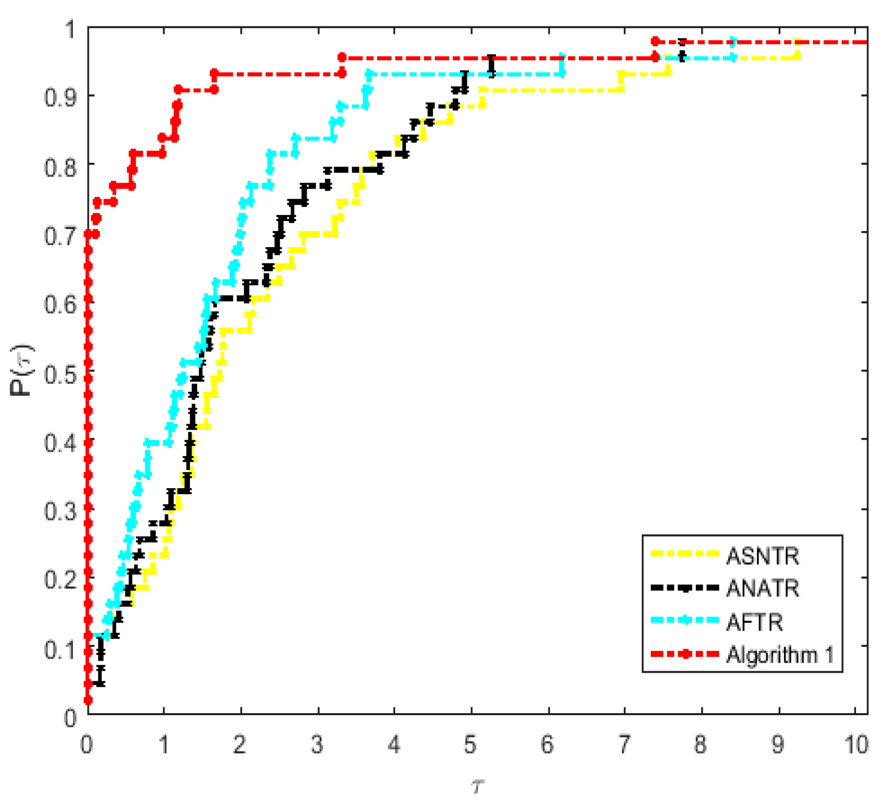
It can be easily seen from Figure 1, Figure 2 and Figure 3 that the new algorithm shows a better performance than the other algorithms from the perspective of the number of function evaluations, the number of gradient evaluations, and running time, especially in contrast to ASNTR. As a general result, we can infer that the new algorithm is more efficient and robust than the other mentioned algorithms in terms of the total number of iterations and running time.
5. Conclusions
In this paper, we combine the nonmonotone adaptive line search strategy with multidimensional filter techniques, and propose a nonmonotone trust region method with a new adaptive radius. Our method possesses the following attractive properties:
(1) The new algorithm is quite different from the standard trust region method; in order to avoid resolving the subproblem, a new nonmonotone Goldstein-type line search is performed in the direction of the rejected trial step.
(2) A new adaptive trust region radius is presented, which decreases the amount of work and computational time. However, full use of the function information for the new trust region radius is not made. A modified trust region ratio is computed which provides more information about evaluating the consistency between the quadratic model and the objective function.
(3) The approximation of the Hessian matrix is updated by the modified BFGS method.
Convergence analysis has shown that the proposed algorithm preserves global convergence as well as superlinear convergence. Numerical experiments were performed on a set of unconstrained optimization test problems in [31]. The numerical results showed that the proposed method is more competitive than the ASNTR, ANATR, and AFTR algorithms for medium-scale problems and large-scale problems with respect to the performance profile explained by Dolan–Moré in [33]. Thus, we can draw the conclusion that the new algorithm works quite well for solving unconstrained optimization problems. In the future, it will be interesting to see the new nonmonotone trust region method used to solve constrained optimization problems and nonlinear equations with constrained conditions. On the other hand, it also will be interesting to combine an improved conjugate gradient algorithm with an improved nonmonotone trust region method to solve many optimization problems.
Author Contributions
Conceptualization, Q.Q.; Writing—original draft, Q.Q.; Methodology, Q.Q; Writing—review and editing, X.D; Resources, X.D. Data curation, X.W; Project administration, X.W; Software, X.W. All authors have read and agreed to the published version of the manuscript.
Funding
This research received no external funding.
Acknowledgments
The authors thank all those who helped improve the quality of the article.
Conflicts of Interest
The authors declare no conflict of interest.
Appendix A
      function [xstar,ystar,fnum,gnum,k,val]=nonmonotone40(x0,N,npro)
      flag=1;
      k=1;
      j=0;
      x=x0;
      n=length(x);
      f(k)=f_test(x,n,npro);
      g=g_test(x,n,npro);
      H=eye(n,n);
      eta1=0.25;
      fnum=1;
      gnum=1;
      flk=f(k);
      p=0;
      delta=norm(g);
      eps=1e-6;
      t=1;
      F(:,t)=x;
      t=t+1;
      while flag
          if (norm(g)<=eps*(1+abs(f(k))))
              flag=0;
              break;
          end
          [d, val] = Trust_q(f(k), g, H, delta);
          faiafa=f_test(x+d,n,npro);
          fnum=fnum+1;
          flk=mmax(f,k-j,k);
          Rk=0.25*flk+0.75*f(k);
          dq = flk- f_test(x,n,npro)- val;
          df=Rk-faiafa;
          rk = df/dq;
          flag_filter=0;
           if rk > eta1
             x1=x+d;
            faiafa=f_test(x1,n,npro);
           else
               g0=g_test(x+d,n,npro);
               for i=1:(t-1)
               gg=g_test(F(:,i),n,npro);
               end
               for l =1:n
                   rg=1/sqrt(n-1);
               if abs(g0(l))<=abs(gg(l))-rg*norm(gg)
                   flag_filter=1;
               end
               end
                 m=0;
                 mk=0;
                rho=0.6;
               sigma=0.25;
          while (m<20)
              if f_test(x+rho^m*d,n,npro)<f_test(x,n,npro )+sigma*rho^m*g'*d
                  mk=m;
                 break;
             end
              m=m+1;
           end
           x1=x+rho^mk*d;
           faiafa=f_test(x1,n,npro);
           fnum=fnum+1;
           p=p+1;
           end
           flag1=0;
           if flag_filter==1
                  flag1=1;
                  g_f2=abs(g);
                   for i=1:t-1
                    g_f1=abs(g_test(F(:,i),n,npro));
                     if g_f1>g_f2
                         F(:,i)=x0;
                     end
                   end
          end
              %%%%%%%%%%%%%%%%%%%%
               if flag1==1
                   F(:,t)=x;
                   t=t+1;
               else
               for i=1:t-1
                                 if F(:,i)==x
                                     F(:,i)=[];
                                     t=t-1;
                                 end
                    end
               end
          dx = x1-x;
          dg=g_test(x1, n,npro)-g;
          if dg'*dx > 0
                  H= H- (H*(dx*dx’) *H)/(dx'*H*dx) + (dg*dg')/(dg'*dx);
          end
           delta=0.5^p*norm(g)^0.75;
           k=k+1;
           f(k)=faiafa;
           j=min ([j+1, M]);
           g=g_test(x1, n,npro);
           gnum=gnum+1;
           x0=x1;
           x=x0;
           p=0;
      end
      val = f(k)+ g'*d + 0.5*d'*H*d;
      xstar=x;
      ystar=f(k);
      end
      function [d, val] = Trust_q(Fk, gk, H, deltak)
      min qk(d)=fk+gk'*d+0.5*d'*Bk*d, s.t.||d|| <= delta
      n = length(gk);
      rho = 0.6;
      sigma = 0.4;
      mu0 = 0.5;
      lam0 = 0.25;
      gamma = 0.15;
      epsilon = 1e-6;
      d0 = ones(n, 1);
      zbar = [mu0, zeros(1, n + 1)]';
      i = 0;
      mu = mu0;
      lam = lam0;
      d = d0;
      while i <= 100
          HB = dah (mu, lam, d, gk, H, deltak);
          if norm(HB) <= epsilon
              break;
          end
          J = JacobiH(mu, lam, d,H, deltak);
          b = psi (mu, lam, d, gk, H, deltak, gamma) *zbar - HB;
          dz = J\b;
          dmu = dz(1);
          dlam = dz(2);
          dd = dz(3 : n + 2);
          m = 0;
          mi = 0;
          while m < 20
              t1 = rho^m;
              Hnew = dah (mu + t1*dmu, lam + t1*dlam, d + t1*dd, gk, H, deltak);
              if norm(Hnew) <= (1 - sigma*(1 - gamma*mu0) *rho^m) *norm(HB)
                  mi = m;
                  break;
              end
              m = m+1;
          end
          alpha = rho^mi;
          mu = mu + alpha*dmu;
          lam = lam + alpha*dlam;
          d = d + alpha*dd;
          i = i + 1;
      end
      val = Fk+ gk'*d + 0.5*d'*H*d;
      end
      function p = phi (mu, a, b)
      p = a + b - sqrt((a - b)^2 + 4*mu^2);
      end
      function HB = dah (mu, lam, d, gk,H, deltak)
      n = length(d);
      HB = zeros (n + 2, 1);
      HB (1) = mu;
      HB (2) = phi (mu, lam, deltak^2 - norm(d)^2);
      HB (3: n + 2) = (H + lam*eye(n)) *d + gk;
      end
      function J = JacobiH(mu, lam, d, H, deltak)
      n = length(d);
      t2 = sqrt((lam + norm(d)^2 - deltak^2)^2 + 4*mu^2);
      pmu = -4*mu/t2;
      thetak = (lam + norm(d)^2 - deltak^2)/t2;
      J= [1,                0,               zeros(1, n);
          pmu,           1 - thetak,  -2*(1 + thetak)*d';
          zeros (n, 1),  d,               H+ lam*eye(n)];
      end
      function si = psi (mu, lam, d, gk,H, deltak, gamma)
      HB = dah (mu, lam, d, gk,H, deltak);
      si = gamma*norm(HB)*min (1, norm(HB));
      end
      Partial test function
        function f = f_test(x,n,nprob)
      %      integer i,iev,ivar,j
      %      real ap,arg,bp,c2pdm6,cp0001,cp1,cp2,cp25,cp5,c1p5,c2p25,c2p625,
      %           c3p5,c25,c29,c90,c100,c10000,c1pd6,d1,d2,eight,fifty,five,
      %           four,one,r,s1,s2,s3,t,t1,t2,t3,ten,th,three,tpi,two,zero
      %      real fvec(50), y(15)
           zero = 0.0e0; one = 1.0e0; two = 2.0e0; three = 3.0e0; four = 4.0e0;
           five = 5.0e0; eight = 8.0e0; ten = 1.0e1; fifty = 5.0e1;
           c2pdm6 = 2.0e-6; cp0001 = 1.0e-4; cp1 = 1.0e-1; cp2 = 2.0e-1;
           cpp2=2.0e-2; cp25 = 2.5e-1; cp5 = 5.0e-1; c1p5 = 1.5e0; c2p25 = 2.25e0;
           c2p625 = 2.625e0; c3p5 = 3.5e0; c25 = 2.5e1; c29 = 2.9e1;
           c90 = 9.0e1; c100 = 1.0e2; c10000 = 1.0e4; c1pd6 = 1.0e6;
           ap = 1.0e-5; bp = 1.0e0;
      if nprob == 1
      % extended rosenbrock function
            f = zero;
            for j = 1: 2: n
               t1 = one - x(j);
               t2 = ten*(x(j+1) - x(j)^2);
               f = f + t1^2 + t2^2;
            end
       elseif nprob == 3
      % Extended White & Holst function
            f = zero;
            for j = 1: 2: n
               t1 = one - x(j);
               t2 = ten*(x(j+1) - x(j)^3);
               f = f + t1^2 + t2^2;
            end
      elseif nprob == 4
      %EXT beale function.
            f=zero;
            for j=1:2: n
              s1=one-x(j+1);
              t1=c1p5-x(j)*s1;
              s2=one-x(j+1) ^2;
              t2=c2p25-x(j)*s2;
              s3 = one - x(j+1) ^3;
              t3 = c2p625 - x(j)*s3;
            f = f+t1^2 + t2^2 + t3^2;
          end
      elseif nprob == 5
      % penalty function i.
            t1 = -cp25;
            t2 = zero;
            for j = 1: n
               t1 = t1 + x(j)^2;
               t2 = t2 + (x(j) - one) ^2;
            end
            f = ap*t2 + bp*t1^2;
      elseif nprob == 6
      % Pert.Quad
            f1=zero;
            f2=zero;
            f=zero;
            for j=1: n
            t=j*x(j)^2;
           f1=t+f1;
      for j=1: n
          t2=x(j);
          f2=f2+t2;
      end
      f=f+f1+1/c100*f2^2;
      elseif nprob == 7
       % Raydan 1
        f=zero;
        for j=1: n
          f1=j*(exp(x(j))-x(j))/ten;
          f=f1+f;
        end
      elseif nprob == 8
      % Raydan 2 function
          f=zero;
          for j=1: n
          ff=exp(x(j))-x(j);
          f=ff+f;
          end
      elseif nprob==9
       % Diagonal 1
          f=zero;
          for j=1: n
           ff=exp(x(j))-j*x(j);
           f=ff+f;
          end
      elseif nprob==10
      % Diagonal 2
      f=zero;
      for j=1: n
          ff=exp(x(j))-x(j)/j;
          f=ff+f;
          x0(j)=1/j;
      end
      elseif nprob==11
      % Diagonal 3
        f=zero;
        for i=1: n
          ff=exp(x(i))-i*sin(x(i));
          f=ff+f;
        end
      elseif nprob==12
       % Hager
      f=zero;
      for j=1: n
           f1=exp(x(j))-sqrt(j)*x(j);
           f=f+f1;
      end
      elseif nprob==13
      %Gen. Trid 1
      f=zero;
      for j=1: n-1
          f1=(x(j)-x(j+1) +one) ^4+(x(j)+x(j+1)-three) ^2;
          f=f+f1;
      end
      elseif nprob==14
      %Extended Tridiagonal 1 function
      f=zero;
      for j=1:2: n
         f1=(x(j)+x(j+1)-three) ^2+(x(j)+x(j+1) +one) ^4;
         f=f1+f;
      end
      elseif nprob==15
      %Extended TET function
      f=zero;
      for j=1:2: n
          f1=exp(x(j)+three*x(j+1)-cp1) + exp(x(j)-three*x(j+1)-cp1) +exp(-x(j)-cp1);
          f=f1+f;
      end
      end
      function g = g_test(x,n,nprob)
      %      integer i,iev,ivar,j
      %      real ap,arg,bp,c2pdm6,cp0001,cp1,cp2,cp25,cp5,c1p5,c2p25,c2p625,
      %     *     c3p5,c19p8,c20p2,c25,c29,c100,c180,c200,c10000,c1pd6,d1,d2,
      %     *     eight,fifty,five,four,one,r,s1,s2,s3,t,t1,t2,t3,ten,th,
      %     *    three,tpi,twenty,two,zero
      %      real fvec(50), y(15)
      %      real float
      %      data zero,one,two,three,four,five,eight,ten,twenty,fifty
      %     *     /0.0e0,1.0e0,2.0e0,3.0e0,4.0e0,5.0e0,8.0e0,1.0e1,2.0e1,
      %     *      5.0e1/
      %      data c2pdm6, cp0001, cp1, cp2, cp25, cp5, c1p5, c2p25, c2p625, c3p5,
      %     *     c19p8, c20p2, c25, c29, c100, c180, c200, c10000, c1pd6
      %     *     /2.0e-6,1.0e-4,1.0e-1,2.0e-1,2.5e-1,5.0e-1,1.5e0,2.25e0,
      %     *      2.625e0,3.5e0,1.98e1,2.02e1,2.5e1,2.9e1,1.0e2,1.8e2,2.0e2,
      %     *      1.0e4,1.0e6/
      %      data ap,bp /1.0e-5,1.0e0/
      %      data y(1),y(2),y(3),y(4),y(5),y(6),y(7),y(8),y(9),y(10),y(11),
      %     *     y (12), y (13), y (14), y (15)
      %     *     /9.0e-4,4.4e-3,1.75e-2,5.4e-2,1.295e-1,2.42e-1,3.521e-1,
      %     *      3.989e-1,3.521e-1,2.42e-1,1.295e-1,5.4e-2,1.75e-2,4.4e-3,
      %     *      9.0e-4/
           zero = 0.0e0; one = 1.0e0; two = 2.0e0; three = 3.0e0; four = 4.0e0;
           five = 5.0e0; eight = 8.0e0; ten = 1.0e1; twenty = 2.0e1; fifty = 5.0e1;
           cpp2=2.0e-2; c2pdm6 = 2.0e-6; cp0001 = 1.0e-4; cp1 = 1.0e-1; cp2 = 2.0e-1;
           cp25 = 2.5e-1; cp5 = 5.0e-1; c1p5 = 1.5e0; c2p25 = 2.25e0; c40=4.0e1;
           c2p625 = 2.625e0; c3p5 = 3.5e0; c25 = 2.5e1; c29 = 2.9e1;
           c180 = 1.8e2; c100 = 1.0e2; c400=4.0e4; c200=2.0e2; c600=6.0e2; c10000 = 1.0e4; c1pd6 = 1.0e6;
           ap = 1.0e-5; bp = 1.0e0; c200 = 2.0e2; c19p8 = 1.98e1;
           c20p2 = 2.02e1;
      if nprob == 1
      %extended rosenbrock function.
         for j = 1: 2: n
               t1 = one - x(j);
               g(j+1) = c200*(x(j+1) - x(j)^2);
               g(j) = -two*(x(j)*g(j+1) + t1);
         end
      elseif nprob == 3
      % Extended White & Holst function
       for j = 1: 2: n
               t1 = one - x(j);
          g(j)=two*t1-c600*(x(j+1)-x(j)^3) *x(j);
          g(j+1) =c200*(x(j+1)-x(j)^3);
       end
      elseif nprob == 4
      % powell badly scaled function.
          for j=1:2: n
            s1 = one - x(j+1);
            t1 = c1p5 - x(j)*s1;
            s2 = one - x(j+1) ^2;
            t2 = c2p25 - x(j)*s2;
            s3 = one - x(j+1) ^3;
            t3 = c2p625 - x(j)*s3;
            g(j) = -two*(s1*t1 + s2*t2 + s3*t3);
            g(j+1) = two*x(j)*(t1 + x(j+1) *(two*t2 + three*x(j+1) *t3));
          end
      elseif nprob == 5
      % penalty function i.
         for j=1: n
            g(j)=four*bp*x(j)*(x(j)^2-cp25) +two*(x(j)-one);
         end
      elseif nprob == 6
        % Perturbed Quadratic function
          f2=zero;
      for j=1: n
          t2=x(j);
          f2=f2+t2;
      end
      for j=1: n
           g(j)=two*j*x(j)+cpp2*f2^2;
      end
      elseif nprob == 7
      % Raydan 1
      for j=1: n
          g(j)=j*(exp(x(j))-one)/ten;
      end
      elseif nprob ==8
      % Raydan 2
      for j=1: n
          g(j)=exp(x(j))-one;
      end
      elseif nprob==9
      % Diagonal 1 function
      for j=1: n
       g(j)=exp(x(j))-j;
      end
      elseif nprob==10
      % Diagonal 2 function
        for j=1: n
          g(j)=exp(x(j))-1/j;
        end
      elseif nprob==11
      % Diagonal 3 function
        for j=1: n
          g(j)=exp(x(j))-j*cos(x(j));
        end
      elseif nprob==12
      % Hager function
        for j=1: n
          g(j)=exp(x(j))-sqrt(j);
        end
      elseif nprob==13
      % Gen. Trid 1
        for j=1:2: n-1
           g(j)=four*(x(j)-x(j+1)+one)^3+two*(x(j)+x(j+1)-three);
           g(j+1)=-four*(x(j)-x(j+1)+one)^3+two*(x(j)+x(j+1)-three);
        end
      elseif nprob==14
      %Extended Tridiagonal 1 function
        for j=1:2: n
          g(j)=two*(x(j)+x(j+1)-three)+four*(x(j)+x(j+1)+one)^3;
          g(j+1)=two*(x(j)+x(j+1)-three)+four*(x(j)+x(j+1)+one)^3;
        end
      elseif nprob==15
      % Extended TET function
      for j=1:2: n
          g(j)=exp(x(j)+three*x(j+1)-cp1)+ exp(x(j)-three*x(j+1)-cp1)-exp(-x(j)-0.1);
          g(j+1) =three*exp(x(j)+three*x(j+1)-cp1)-three*exp(x(j)-three*x(j+1)-cp;
      end
      tic;
      npro=1;
      %Extended Rosenbrock
      if npro==1
          x0=zeros (500,1);
          for i=1:2:500
              x0(i)=-1.2;
              x0(i+1) =1;
          end
      %Generalized Rosenbrock
      elseif npro==2
       x0=zeros (1000,1);
          for i=1:2:1000
              x0(i)=-1.2;
              x0(i+1) =1;
          end
      %Extended White & Holst function
      elseif npro==3
        x0=zeros (500,1);
          for i=1:2:500
              x0(i)=-1.2;
              x0(i+1) =1;
          end
      %Extended Beale
      elseif npro==4
         x0=zeros (500,1);
         for i=1:2:500
             x0(i)=1;
             x0(i)=0.8;
         end
       %Penalty
      elseif npro==5
          x0=zeros (500,1);
          for i=1:500
          x0(i)=i;
          end
      % Perturbed Quadratic function
      elseif npro==6
          x0=0.5*ones (36,1);
      % Raydan 1
      elseif npro == 7
          x0=ones (100,1);
      %Raydan 2
      elseif npro==8
         x0=ones (500,1);
      %Diagonal 1 function
      elseif npro==9
        x0=0.5*ones (500,1);
      %Diagonal 2 function
       elseif npro==10
         x0=zeros (500,1);
         for i=1:500
          x0(i)=1/i;
         end
      %Diagonal 3 function
      elseif npro==11
          x0=ones (500,1);
      % Hager function
       elseif npro==12
          x0=ones (500,1);
      %Gen. Trid 1
       elseif npro==13
          x0=2*ones (500,1);
      %Extended Tridiagonal 1 function
       elseif npro==14
          x0=2*ones (500,1);
      %Extended TET function
       elseif npro==15
          x0=0.1*ones (500,1);
      end
      N=5;
      [xstar,ystar,fnum,gnum,k,val]=nonmonotone40(x0,N,npro);
      fprintf('%d, %d,%d',fnum,gnum,val);
      xstar;
      ystar;
      toc
References
- Jiang, X.Z.; Jian, J.B. Improved Fletcher-Reeves and Dai-Yuan conjugate gradient methods with the strong Wolfe line search. J. Comput. Appl. Math. 2019, 328, 525–534. [Google Scholar] [CrossRef]
- Fatemi, M. A new efficient conjugate gradient method for unconstrained optimization. J. Comput. Appl. Math. 2016, 300, 207–216. [Google Scholar] [CrossRef]
- Andrei, N. New hybrid conjugate gradient algorithms for unconstrained optimization. Encycl. Optim. 2009, 141, 2560–2571. [Google Scholar]
- Gao, H.; Zhang, H.B.; Li, Z.B. A nonmonotone inexact Newton method for unconstrained optimization. Optim. Lett. 2017, 11, 947–965. [Google Scholar] [CrossRef]
- Kenji, U.; Nobuo, Y. A regularized Newton method without line search for unconstrained optimization. Comput. Optim. Appl. 2014, 59, 321–351. [Google Scholar]
- Xue, Y.Q.; Liu, H.W.; Liu, H.Z. An improved nonmonotone adaptive trust region method. Appl. Math. 2019, 3, 335–350. [Google Scholar] [CrossRef]
- Rezaee, S.; Babaie-Kafaki, S. A modified nonmonotone trust region line search method. J. Appl. Math. Comput. 2017. [CrossRef]
- Wang, X.Y.; Ding, X.F.; Qu, Q. A New Filter Nonmonotone Adaptive Trust Region Method for Unconstrained Optimization. Symmetry 2020, 12, 208. [Google Scholar] [CrossRef] [Green Version]
- Nocedal, J.; Yuan, Y. Combining trust region and line search techniques. Adv. Nonlinear Program. 1998, 153–175. [Google Scholar]
- Michael, G.E. A Quasi-Newton Trust Region Method. Math. Program. 2004, 100, 447–470. [Google Scholar] [CrossRef]
- Li, C.Y.; Zhou, Q.H.; Wu, X. A Non-Monotone Trust Region Method with Non-Monotone Wolfe-Type Line Search Strategy for Unconstrained Optimization. J. Appl. Math. Phys. 2015, 3, 707–712. [Google Scholar] [CrossRef] [Green Version]
- Zhang, H.C.; Hager, W.W. A nonmonotone line search technique and its application to unconstrained optimization. SIAM J. Optim. 2004, 14, 1043–1056. [Google Scholar] [CrossRef] [Green Version]
- Chamberlain, R.M.; Powell, M.J.D.; Lemarechal, C.; Pedersen, H.C. The watchdog technique for forcing convergence in algorithm for constrained optimization. Math. Program. Stud. 1982, 16, 1–17. [Google Scholar]
- Grippo, L.; Lamparillo, F.; Lucidi, S. A nonmonotone line search technique for Newton’s method. Siam J. Numer. Anal. 1986, 23, 707–716. [Google Scholar] [CrossRef]
- Cui, Z.C.; Wu, B.; Qu, S.J. Combining nonmonotone conic trust region and line search techniques for unconstrained optimization. J. Comput. Appl. Math. 2011, 235, 2432–2441. [Google Scholar] [CrossRef] [Green Version]
- Ahookhoosh, M.; Amini, K.; Peyghami, M. A nonmonotone trust region line search method for large scale unconstrained optimization. Appl. Math. Model. 2012, 36, 478–487. [Google Scholar] [CrossRef]
- Sartenaer, A. Automatic determination of an initial trust region in nonlinear programming. SIAM J. Sci. Comput. 1997, 18, 1788–1803. [Google Scholar] [CrossRef] [Green Version]
- Zhang, X.S.; Zhang, J.L.; Liao, L.Z. An adaptive trust region method and its convergence. Sci. China 2002, 45, 620–631. [Google Scholar] [CrossRef] [Green Version]
- Zhou, S.; Yuan, G.L.; Cui, Z.R. A new adaptive trust region algorithm for optimization problems. Acta Math. Sci. 2018, 38B, 479–496. [Google Scholar]
- Kimiaei, M. A new class of nonmonotone adaptive trust-region methods for nonlinear equations with box constraints. Calcolo 2017, 54, 769–812. [Google Scholar] [CrossRef]
- Amini, K.; Shiker Mushtak, A.K.; Kimiaei, M. A line search trust-region algorithm with nonmonotone adaptive radius for a system of nonlinear equations. Q. J. Oper. Res. 2016, 4, 132–152. [Google Scholar] [CrossRef]
- Peyghami, M.R.; Tarzanagh, D.A. A relaxed nonmonotone adaptive trust region method for solving unconstrained optimization problems. Comput. Optim. Appl. 2015, 61, 321–341. [Google Scholar] [CrossRef]
- Fletcher, R.; Leyffer, S. Nonlinear programming without a penalty function. Math. Program. 2002, 91, 239–269. [Google Scholar] [CrossRef]
- Gould, N.I.; Sainvitu, C.; Toint, P.L. A filter-trust-region method for unconstrained optimization. Siam J. Optim. 2005, 16, 341–357. [Google Scholar] [CrossRef] [Green Version]
- Wächter, A.; Biegler, L.T. Line search filter methods for nonlinear programming and global convergence. SIAM J. Optim. 2005, 16, 1–31. [Google Scholar] [CrossRef]
- Miao, W.H.; Sun, W. A filter trust-region method for unconstrained optimization. Numer. Math. J. Chin. Univ. 2007, 19, 88–96. [Google Scholar]
- Zhang, Y.; Sun, W.; Qi, L. A nonmonotone filter Barzilai-Borwein method for optimization. Asia Pac. J. Oper. Res. 2010, 27, 55–69. [Google Scholar] [CrossRef]
- Conn, A.R.; Gould, N.I.M.; Toint, P.L. Trust-Region Methods, MPS-SIAM Series on Optimization; SIAM: Philadelphia, PA, USA, 2000. [Google Scholar]
- Gu, N.Z.; Mo, J.T. Incorporating Nonmonotone Strategies into the Trust Region for Unconstrained Optimization. Comput. Math. Appl. 2008, 55, 2158–2172. [Google Scholar] [CrossRef] [Green Version]
- Pang, S.M.; Chen, L.P. A new family of nonmonotone trust region algorithm. Math. Pract. Theory. 2011, 10, 211–218. [Google Scholar]
- Andrei, N. An unconstrained optimization test functions collection. Environ. Sci. Technol. 2008, 10, 6552–6558. [Google Scholar]
- Toint, P.L. Global convergence of the partitioned BFGS algorithm for convexpartially separable optimization. Math. Program. 1986, 36, 290–306. [Google Scholar] [CrossRef]
- Dolan, E.D.; Moré, J.J. Benchmarking optimization software with performance profiles. Math. Program. 2002, 91, 201–213. [Google Scholar] [CrossRef]
Figure 1.
Performance profile for the number of function evaluations ().

Figure 2.
Performance profile for the number of gradient evaluations ().

Figure 3.
Performance profile for running time (CPU).


Table 1.
Numerical comparisons on a subset of test problems. ASNTR: The standard nonmonotone trust region algorithm of Pang et al.; ANATR: The nonmonotone adaptive trust region algorithm of Ahookhoosh et al.; AFTR: The multidimensional filter trust region algorithm of Wang et al.
Table 1.
Numerical comparisons on a subset of test problems. ASNTR: The standard nonmonotone trust region algorithm of Pang et al.; ANATR: The nonmonotone adaptive trust region algorithm of Ahookhoosh et al.; AFTR: The multidimensional filter trust region algorithm of Wang et al.
| Problem | |||||||||
|---|---|---|---|---|---|---|---|---|---|
| ASNTR | CPU | ANATR | CPU | AFTR | CPU | Algorithm 1 | CPU | ||
| Extended Rosenbrock | 500 | 2649/1326 | 1867.254 | 1071/840 | 1545.386 | 547/387 | 642.091 | 86/47 | 70.369 |
| Extended White and Holst function | 500 | 13/7 | 26.788 | 5/3 | 6.524 | 5/3 | 2.125 | 3/2 | 0.218 |
| Extended Beale | 500 | 29/15 | 4.386 | 43/22 | 15.351 | 40/36 | 8.532 | 22/17 | 2.953 |
| Penalty i | 500 | 13/8 | 32.186 | 5/3 | 6.593 | 7/4 | 2.176 | 3/2 | 0.171 |
| Pert.Quad | 36 | 153/80 | 0.5523 | 128/67 | 0.4704 | 101/73 | 0.8631 | 86/45 | 0.167 |
| Raydan 1 | 100 | 26/14 | 0.862 | 130/98 | 2.263 | 208/105 | 3.5009 | 82/42 | 0.923 |
| Raydan 2 | 500 | 13/8 | 0.9660 | 13/8 | 0.9966 | 11/6 | 0.9549 | 9/5 | 0.780 |
| Diadonal 1 | 500 | 82/42 | 40.591 | 1459/812 | 1957.794 | 59/43 | 21.091 | 21/11 | 9.107 |
| Diadonal 2 | 500 | 4765/3529 | 1532.176 | 251/198 | 106.641 | 390/201 | 43.252 | 2116/1062 | 430.600 |
| Diagonal 3 | 500 | 1634/933 | 1822.091 | 1389/766 | 1536.226 | 349/288 | 327.056 | 201/101 | 88.049 |
| Hager | 500 | 42/23 | 30.258 | 1418/760 | 270.837 | 87/46 | 45.342 | 51/26 | 14.278 |
| Generalized Tridiagonal 1 | 500 | 63/32 | 5.6490 | 53/28 | 8.349 | 46/24 | 13.419 | 70/36 | 11.163 |
| Extended Tridiagonal 1 | 500 | 25/13 | 0.9857 | 25/13 | 3.448 | 14/10 | 3.2337 | 8/7 | 0.823 |
| Extended TET | 500 | 15/8 | 4.2638 | 15/9 | 1.632 | 17/9 | 2.5044 | 17/9 | 1.452 |
| Diadonal 4 | 500 | 7/4 | 0.3293 | 7/4 | 0.857 | 9/8 | 4.0362 | 5/4 | 0.419 |
| Diadonal 5 | 500 | 106/54 | 43.3048 | 134/112 | 57.032 | 127/106 | 41.096 | 155/79 | 19.024 |
| Diadonal 7 | 1000 | 96/78 | 29.197 | 88/73 | 22.309 | 34/15 | 10.265 | 19/15 | 2.561 |
| Diadonal 8 | 1000 | 159/122 | 18.542 | 133/126 | 43.067 | 76/36 | 6.781 | 27/21 | 1.550 |
| Extended Him | 1000 | 35/18 | 7.150 | 30/16 | 17.975 | 108/87 | 514.843 | 28/18 | 22.572 |
| Full Hessian FH3 | 1000 | 11/6 | 1.755 | 11/6 | 5.555 | 17/13 | 5.1472 | 11/6 | 3.912 |
| Extended BD1 | 1000 | 43/25 | 61.358 | 30/16 | 17.9073 | 35/19 | 23.4119 | 30/19 | 26.971 |
| Quadratic QF1 | 1000 | 287/195 | 157.332 | 293/219 | 0.259 | 400/274 | 87.043 | 197/99 | 43.280 |
| FLETCHCR34 | 1000 | 847/505 | 67.511 | 345/225 | 100.676 | 24/16 | 73.265 | 8/5 | 33.145 |
| ARWHEAD | 1000 | 47/24 | 38.4334 | 29/16 | 24.338 | 64/41 | 38.552 | 24/17 | 18.299 |
| NONDIA | 1000 | 197/104 | 96.176 | 92/47 | 56.432 | 33/23 | 34.726 | 51/35 | 22.318 |
| DQDRTIC | 1000 | 23/12 | 52.102 | 36/19 | 40.949 | 46/37 | 86.265 | 22/15 | 16.526 |
| EG2 | 1000 | 55/30 | 79.991 | 28/16 | 16.042 | 19/19 | 14.169 | 51/26 | 32.424 |
| Broyden Tridiagonal | 1000 | 1978/1488 | 1545.221 | 1553/1288 | 1266.076 | 1226/987 | 782.560 | 754/646 | 456.105 |
| Almost Perturbed Quadratic | 1600 | 2548/2267 | 1960.433 | 2118/1829 | 1543.253 | 1078/718 | 1067.206 | 657/425 | 279.316 |
| Perturbed Tridiagonal Quadratic | 3000 | 1342/1025 | 1672.434 | 1132/876 | 1033.255 | 745/552 | 835.265 | 453/357 | 572.371 |
| DIXMAANA | 3000 | 576/463 | 132.240 | 223/198 | 88.211 | 378/320 | 108.452 | 209/165 | 78.542 |
| DIXMAANB | 3000 | 248/201 | 64.215 | 165/122 | 40.233 | 67/56 | 25.109 | 48/32 | 37.120 |
| DIXMAANC | 3000 | 279/197 | 177.221 | 246/167 | 134.272 | 95/43 | 30.140 | 58/24 | 19.011 |
| Extended DENSCH | 3000 | 673/418 | 476.214 | 533/388 | 309.605 | 254/105 | 199.421 | 87/42 | 219.167 |
| SINCOS | 3000 | 2067/1554 | 1045.301 | 1653/1274 | 836.022 | 337/233 | 472.032 | 275/141 | 165.665 |
| HIMMELH | 3000 | 967/721 | 526.211 | 506/349 | 255.629 | 197/196 | 109.276 | 45/32 | 40.127 |
| BIGGSB1 | 3000 | 3760/2045 | 2321.509 | 2254/1886 | 1308.227 | 1836/1025 | 904.234 | 4051/2381 | 1987.456 |
| ENGVAL1 | 3000 | 1784/1087 | 1643.092 | 587/423 | 960.421 | 63/43 | 243.840 | 58/32 | 167.991 |
| BDEXP | 3000 | 2259/1876 | 978.432 | 1342/978 | 832.013 | 172/137 | 385.439 | 67/43 | 59.276 |
| INDEF | 3000 | 325/209 | 2430.215 | 178/156 | 1023.211 | 34/31 | 721.343 | 19/11 | 479.263 |
| NONSCOMP | 3000 | 264/107 | 1742.856 | 96/47 | 1389.123 | 34/18 | 921.324 | 22/14 | 679.120 |
| QUARTC | 3000 | 167/123 | 643.254 | 332/289 | 921.313 | 22/20 | 425.995 | 67/54 | 356.762 |
© 2020 by the authors. Licensee MDPI, Basel, Switzerland. This article is an open access article distributed under the terms and conditions of the Creative Commons Attribution (CC BY) license (http://creativecommons.org/licenses/by/4.0/).
Share and Cite
MDPI and ACS Style
Qu, Q.; Ding, X.; Wang, X. A Filter and Nonmonotone Adaptive Trust Region Line Search Method for Unconstrained Optimization. Symmetry 2020, 12, 656. https://doi.org/10.3390/sym12040656
AMA Style
Qu Q, Ding X, Wang X. A Filter and Nonmonotone Adaptive Trust Region Line Search Method for Unconstrained Optimization. Symmetry. 2020; 12(4):656. https://doi.org/10.3390/sym12040656
Chicago/Turabian StyleQu, Quan, Xianfeng Ding, and Xinyi Wang. 2020. "A Filter and Nonmonotone Adaptive Trust Region Line Search Method for Unconstrained Optimization" Symmetry 12, no. 4: 656. https://doi.org/10.3390/sym12040656
Note that from the first issue of 2016, this journal uses article numbers instead of page numbers. See further details here.