MHD Boundary Layer Flow of Carreau Fluid over a Convectively Heated Bidirectional Sheet with Non-Fourier Heat Flux and Variable Thermal Conductivity

Abstract

In the present exploration, instead of the more customary parabolic Fourier law, we have adopted the hyperbolic Cattaneo–Christov (C–C) heat flux model to jump over the major hurdle of “parabolic energy equation”. The more realistic three-dimensional Carreau fluid flow analysis is conducted in attendance of temperature-dependent thermal conductivity. The other salient impacts affecting the considered model are the homogeneous-heterogeneous (h-h) reactions and magnetohydrodynamic (MHD). The boundary conditions supporting the problem are convective heat and of h-h reactions. The considered boundary layer problem is addressed via similarity transformations to obtain the system of coupled differential equations. The numerical solutions are attained by undertaking the MATLAB built-in function bvp4c. To comprehend the consequences of assorted parameters on involved distributions, different graphs are plotted and are accompanied by requisite discussions in the light of their physical significance. To substantiate the presented results, a comparison to the already conducted problem is also given. It is envisaged that there is a close correlation between the two results. This shows that dependable results are being submitted. It is noticed that h-h reactions depict an opposite behavior versus concentration profile. Moreover, the temperature of the fluid augments for higher values of thermal conductivity parameters.

1. Introduction

Non-Newtonian fluids have gained substantial attention of researchers and scientists owing to their widespread applications. A number of examples like apple sauce, chyme, emulsions, mud, soaps, shampoos and blood at low shear stress may be quoted as non-Newtonian fluids. Existing literature does not facilitate us to identify a single relation that exhibits numerous physiognomies of non-Newtonian fluids. This is why a variety of mathematical models have been suggested, as deemed appropriate, to the requirement. The viscosity of the fluid plays a vital role in the chemical engineering industry. In case of generalized Newtonian fluids, viscosity is dependent on shear stress. In some fluids, a change up to two to three orders in magnitude may not make a visible effect in some fluids, but its impact can’t be ignored particularly in polymer industry and lubrication processes. Bird et al. [1] presented the idea of generalized Newtonian fluids with the idea that the viscosity fluctuates with the shear rate. Fluid flows over a solid surface have been frequently studied and the reports revealed that surface forces become significant on a micro level and lead to the enhanced fluid viscosity due to fluid layering [2,3,4,5]. The major shortcoming of the Power-law model is that it does not properly address the viscosity in case of very low or high shear rates. To overcome this hurdle, the Carreau fluid model is introduced [6]. Contrary to the Power law model, the viscosity remains finite as the shear rate vanishes. This is why the constitutive relation for the Carreau fluid model is more appropriate in case of free surface flows. Owing to such important characteristics, the Carreau fluid model has attracted researchers for many years. Chhabra and Uhlherr [7] deliberated the Carreau fluid flow over the spheres and this concept was extended by Bush and Phan-Thein [8]. The squeezing Carreau fluid flow past sphere is examined by Uddin et al. [9]. Tshehla [10] deliberated the flow of the Carreau fluid over an inclined plane. The nonlinear radiation impact on the 3D Carreau fluid flow was deliberated by Khan et al. [11]. Khan et al. [12] obtained the solution of the Carreau nanofluid flow analytically with entropy generation. Similar explorations discussing Carreau fluid flow may be found at [13,14,15] and many therein.

Flows under the influence of magnetohydrodynamics (MHD) have a wide range of applications including thermal insulators, blood flow measurements, petroleum and polymer technologies, nuclear reactors and MHD generators. Taking into account all such applications, many researchers have examined the flows stimulated by magnetohydrodynamics. Waqas et al. [16] conversed micropolar fluid’s flow with the effect of convective boundary condition and magnetohydrodynamics. He also considered effects of viscous dissipation and mixed convection. Ramzan et al. [17] deliberated the series solution of micropolar fluid flow in attendance of MHD, partial slip and convective boundary condition over a porous stretching sheet. Besthapu et al. [18] calculated the numerical solution of double stratification nanofluid flow with MHD and viscous dissipation using the finite element method past an exponentially stretching sheet. Khan and Azam [19] explored the flow of Carreau nanofluid under the influence of magnetohydrodynamic using a numerical technique named bvp4c. Turkyilmazoglu [20] examined the exact solution of micropolar fluid flow with the mixed convection and magnetohydrodynamic past a permeable heated/cooled deformable plate. Hayat et al. [21] premeditated the flow of Oldroyd-B nanofluid in attendance of MHD and heat generation/absorption using Optimal Homotopy analysis method HAM. Some recent attempts highlighting effects of magnetohydrodynamic may be found at [22,23,24,25].

The importance of heat transfer is fundamental in many engineering processes like nuclear reactors, fuel cells, and microelectronics. Thermal conductivity is considered to be constant in all such procedures. Nevertheless, the requirement of variable characteristics is fundamental. A variation from $0^{°}$F to ${400}^{°}$F [26] in temperature is observed in such cases. Fourier law of heat conduction [27] has been a customary gauge for years in heat transfer applications. However, a major drawback of parabolic energy equation experiences a disruption in the beginning which prevails throughout the entire process, which forces the researchers to look for some modification to Fourier’s law. Cattaneo [28] proposed an improved Fourier’s law by instituting a thermal relaxation term. Later, Oldroyd’s upper-convected derivatives [29] are considered as an alternative to the thermal relaxation time in Cattaneo’s model. Recent attempts in various scenarios with an emphasis on C–C flux model may encompass a study by Ramzan et al. [30], highlighting effects of the 2D third grade-fluid flow accompanying Cattaneo–Christov heat flux and magnetohydrodynamics. Flow analysis is done in the presence of h-h reactions and convective boundary condition. Hayat et al. [31] found an analytical solution of Jeffrey fluid flow past a stretched cylinder with the effect of C–C heat flux and thermal stratification. Sui et al. [32] studied upper-convected Maxwell nanofluid flow with C–C heat flux and slip boundary condition past a linearly stretched sheet. Liu et al. [33] discussed a fractional C–C flux model numerically where the fractional derivative is represented by a weight coefficient.

Many chemical reactions necessitate the presence of h-h reactions. Fewer of these reactions act at a slow pace, whereas some absolutely not except in the attendance of the catalyst. These reactions are involved in many scenarios like fibrous insulations, production of polymers and ceramics, and air and water pollution. The heterogeneous reactions cover the complete phase evenly and is found in solid phase. Nevertheless, the homogeneous reactions are covered by catalysis and combustion. The homogeneous catalyst occurs in liquid and gaseous states but heterogeneous catalyst exists in solid form. The latest research discussing the h-h reactions effects may comprise the study by Kumar et al. [34] who examined the irreversibility process with h-h reactions of the flow of carbon nanotubes based nanofluid past a bi-directional stretched surface. The flow with h-h reactions of Blasius nanofluid is pondered by Xu [35]. Sithole et al. [36] used a Bivariate spectral local linearization method to investigate the effects of h-h reactions on the flow of time dependent micropolar nanofluid past a stretched surface. The numerical simulations are conducted for h-h reactions and nonlinear thermal radiation past a 3D crossfluid flow with MHD by Khan et al. [37]. In a gravity driven nanofluid film flow, the effects of h-h reactions with mixed convection are deliberated by Rasees et al. [38]. Ramzan et al. [39,40] highlighted the time dependent nanofluid squeezing flow with carbon nanotubes under the influence of h-h reactions and C–C heat flux, and in Micropolar nanofluid flow with thermal radiation past a nonlinear stretched surface and many therein [40,41,42,43,44,45].

In all the aforementioned literature surveys, it is observed that either the effect of only C–C heat flux or h-h reactions have been discussed in various geometries. Even if the simultaneous effects of C–C heat flux and h-h reactions have been discussed, it is in the two-dimensional case. However, much less literature is available featuring effects of both C–C and h-h reactions in 3D models. The present study discusses the 3D Carreau fluid model in attendance of temperature-dependent thermal conductivity, C–C heat flux and h-h reactions accompanied by the impact of convective heat with h-h boundary conditions. A MATLAB built-in bvp4c routine is betrothed to obtain series solutions. Graphs are drawn depicting effects of pertinent parameters on involved distributions. Validation of presented results in the limiting case is also an additional feature of this exploration.

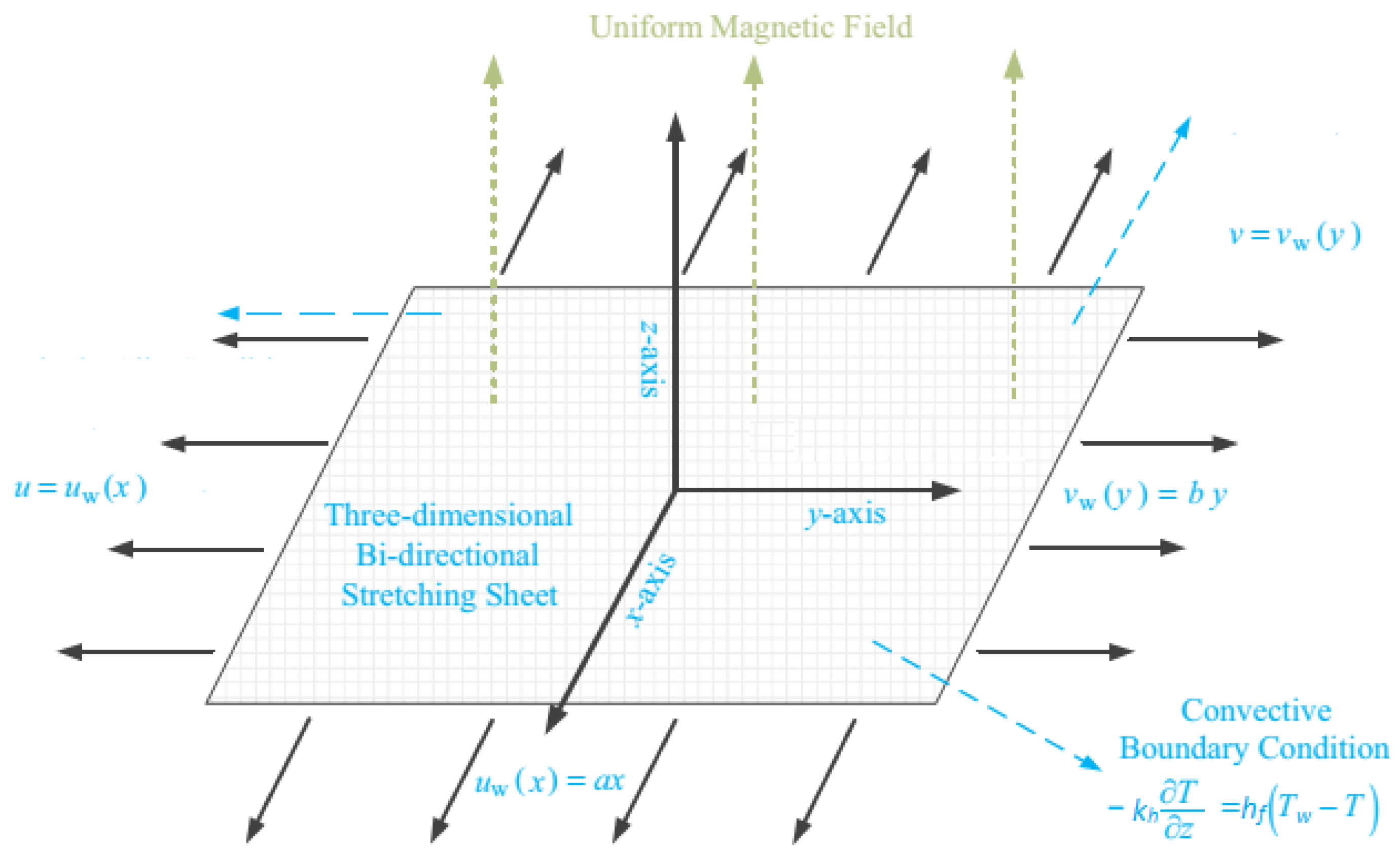
2. Mathematical Formulation

Let us presume a 3D flow of Carreau fluid in x- and y-directions with respective velocities $u=u_w\left(x\right)=cx$ and $v=v_w\left(y\right)=dy$ occupying the region $z=0$ under the influence of C–C heat flux and variable thermal conductivity past a bidirectional stretching surface as shown in Figure 1. Flow analysis is performed subject to h-h reactions with magnetohydrodynamics. Temperature at the surface $T_w$ is considered to be more than the temperature away from the surface $T_{\infty }$. A magnetic field with strength $B_o$ is introduced along the z-axis. Electric and Hall effects are ignored. Small Reynolds number’s assumption needs to omit an induced magnetic field. For two chemical species A and B, analysis is performed in the presence of h-h reactions. For homogeneous reaction, the cubic autocatalysis is epitomized by the following expression [46]:

$$A+2B\to 3B,rate=k_{c}a{b}^2.$$

(1)

However, on the catalyst surface, the first order isothermal reaction is given by:

$$A\to B,rate=k_{s}a.$$

(2)

For both the h-h reaction processes, it is assumed that temperature is constant. Governing equations that abide by the above mentioned assumptions are given below:

$$u_x+v_y+w_z=0,$$

(3)

$$\begin{array}{c}u{u}_x+v{u}_y+w{u}_z=\nu u_{zz}\left[{\beta }^{*}+\left(1-{\beta }^{*}\right){\left\{1+{\mathrm{\Gamma }}^2{\left(u_z\right)}^2\right\}}^{\frac{n-1}{2}}\right]-\frac{\sigma B_o^2}{\rho }u\\ +\nu \left(n-1\right)\left(1-{\beta }^{*}\right){\mathrm{\Gamma }}^2\left(u_{zz}\right){\left(u_z\right)}^2{\left\{1+{\mathrm{\Gamma }}^2{\left(u_z\right)}^2\right\}}^{\frac{n-3}{2}},\end{array}$$

(4)

$$\begin{array}{c}u{v}_x+v{v}_y+w{v}_z=\nu v_{zz}\left[{\beta }^{*}+\left(1-{\beta }^{*}\right){\left\{1+{\mathrm{\Gamma }}^2{\left(v_z\right)}^2\right\}}^{\frac{n-1}{2}}\right]-\frac{\sigma B_o^2}{\rho }v\\ +\nu \left(n-1\right)\left(1-{\beta }^{*}\right){\mathrm{\Gamma }}^2\left(v_{zz}\right){\left(v_z\right)}^2{\left\{1+{\mathrm{\Gamma }}^2{\left(v_z\right)}^2\right\}}^{\frac{n-3}{2}},\end{array}$$

(5)

$$\rho C_P\mathbf{V}.\nabla T=-\nabla .\mathbf{q},$$

(6)

$$u{a}_x+v{a}_y+w{a}_z=D_A{a}_{zz}-k_{c}a{b}^2,$$

(7)

$$u{b}_x+v{b}_y+w{b}_z=D_B{b}_{zz}+k_{c}a{b}^2,$$

(8)

with $\mathbf{q}$ being the heat flux satisfying the relation

$$\mathbf{q}+K_1\left({\mathbf{q}}_t+\mathbf{V}.\nabla \mathbf{q}-\mathbf{q}.\nabla \mathbf{V}+\left(\nabla .\mathbf{V}\right)\mathbf{q}\right)=-\nabla \left(\alpha T\right).$$

(9)

Using the fluid’s incompressibility condition and Christov [29], Equations (6) and (9) take the following form after omission of $\mathbf{q}$:

$$u{T}_x+v{T}_y++w{T}_z=\frac{1}{\rho C_P}{\left(\alpha T_z\right)}_z,$$

$$-K_1\left(\begin{array}{c}{u}^2{T}_{xx}+v^2{T}_{yy}+w^2{T}_{zz}+2uv{T}_{xy}\\ +2vw{T}_{yz}+2uw{T}_{xz}+\left(u{u}_x+v{u}_y+w{u}_z\right)T_x+\\ \left(u{v}_x+v{v}_y+w{v}_z\right)T_y+\left(u{w}_x+v{w}_y+w{w}_z\right)T_z\end{array}\right).$$

(10)

The supporting boundary conditions to the given model are

$$u=u_w\left(x\right)=cx,v=v_w\left(y\right)=dy,w=0,$$

$$-k_h{T}_z=h_f\left(T_w-T\right),D_A{a}_z=k_{s}a,D_B{b}_z=-k_{s}a,atz=0,$$

$$u\to 0,v\to 0,a\to a_o,b\to 0,T\to T_{\infty }asz\to \infty ,$$

(11)

considering temperature dependent thermal conductivity $ϵ=\frac{k_w-k_{\infty }}{k_{\infty }}$ as defined in [47].

Taking into account the transformations

$$\begin{array}{c}u=cx{f}^{\prime }\left(\eta \right),v=cy{g}^{\prime }\left(\eta \right),w=-\sqrt{c\nu }\left(f\left(\eta \right)+g\left(\eta \right)\right),\alpha ={\alpha }_{\infty }\left(1+ϵ\theta \right),\\ \theta \left(\eta \right)=\frac{T-T_{\infty }}{T_w-T_{\infty }},\eta =\sqrt{\frac{c}{\nu }}z,a=a_0\varphi \left(\eta \right),b=a_{0}h\left(\eta \right).\end{array}$$

(12)

The requirement of Equation (3) is met inevitably, whereas Equations (4), (5), (7), (8), (10) and (11) take the following form:

$$\left[{\beta }^{*}+\left(1-{\beta }^{*}\right){\left\{1+W{e}_1^2{\left(f^{″}\right)}^2\right\}}^{\frac{n-3}{2}}\left\{1+nW{e}_1^2{\left(f^{″}\right)}^2\right\}\right]f^{‴}+\left(f+g\right)f^{″}-{f^{\prime }}^2-M^2{f}^{\prime }=0,$$

(13)

$$\left[{\beta }^{*}+\left(1-{\beta }^{*}\right){\left\{1+W{e}_2^2{\left(g^{″}\right)}^2\right\}}^{\frac{n-3}{2}}\left\{1+nW{e}_2^2{\left(g^{″}\right)}^2\right\}\right]g^{‴}+\left(f+g\right)g^{″}-{g^{\prime }}^2-M^2{g}^{\prime }=0,$$

(14)

$$\left(1+ϵ\theta \right){\theta }^{″}+ϵ{{\theta }^{\prime }}^2+Pr\left(f+g\right){\theta }^{\prime }-Pr{\lambda }_1\left({\left(f+g\right)}^2{\theta }^{″}+\left(f+g\right)\left(f^{\prime }+g^{\prime }\right){\theta }^{\prime }\right)=0,$$

(15)

$${\varphi }^{″}+Sc\left(f+g\right){\varphi }^{\prime }-Sc{\gamma }_1\varphi h^2=0,$$

(16)

$$\zeta h^{″}+Sc\left(f+g\right)h^{\prime }+Sc{\gamma }_1\varphi h^2=0,$$

(17)

$$\begin{array}{c}f\left(0\right)=0,f^{\prime }\left(0\right)=1,g\left(0\right)=0,g^{\prime }\left(0\right)=\lambda ,\\ {\varphi }^{\prime }\left(0\right)={\gamma }_2\varphi \left(0\right),{\theta }^{\prime }\left(0\right)=-\delta \left(1-\theta \left(0\right)\right),\\ \zeta h^{\prime }\left(0\right)=-{\gamma }_2\varphi \left(0\right),f^{\prime }(\infty )\to 0,f^{″}\left(\infty \right)\to 0,g^{\prime }\left(\infty \right)\to 0,\\ g^{″}\left(\infty \right)\to 0,\theta \left(\infty \right)\to 0,\varphi \left(\infty \right)\to 1.\end{array}$$

(18)

Different parameters used in the above equations are defined as follows:

$$\begin{array}{c}{\gamma }_1=\frac{k_c{a}_0^2}{c},{\gamma }_2=\frac{k}{D_A{a}_0}\sqrt{\frac{v}{c}},Sc=\frac{\nu }{D_A},Pr=\frac{\mu C_p}{k},\lambda =\frac{d}{c},\\ W{e}_1=\sqrt{\frac{c{\mathrm{\Gamma }}^2{U}_w^2}{\nu }},W{e}_2=\sqrt{\frac{c{\mathrm{\Gamma }}^2{V}_w^2}{\nu }},{\lambda }_1=K_{1}c,\zeta =\frac{D_B}{D_A},\delta =\frac{h_f}{k}\sqrt{\frac{\nu }{c}},M^2=\frac{\sigma B_o^2}{c\rho }.\end{array}$$

(19)

The expectation as in most applications that coefficients of chemical species A and B are of equivalent magnitude lead us to make a supplementary presumption that diffusion coefficients $D_A$ and $D_B$ are equivalent i.e., $\zeta =1,$ [46]. Thus, we get:

$$\varphi \left(\eta \right)+h\left(\eta \right)=1.$$

(20)

Now, Equations (16) and (17) take the following form:

$${\varphi }^{″}+Sc\left(f+g\right){\varphi }^{\prime }-Sc{\gamma }_1\varphi {\left(1-\varphi \right)}^2=0,$$

(21)

with boundary conditions

$${\varphi }^{\prime }\left(0\right)={\gamma }_2\varphi \left(0\right),\varphi (\infty )=1.$$

(22)

The skin friction coefficient in dimensional form is

$$C_{fx}=\frac{{\tau }_{xz}}{\rho U_w^2\left(x\right)},C_{fy}=\frac{{\tau }_{yz}}{\rho u_w^2\left(y\right)}.$$

(23)

Dimensionless forms of Skin friction coefficient is

$$\begin{array}{ccc}\hfill C_{fx}{Re}_x^{1/2}& =& f^{″}\left(0\right)\left[{\beta }^{*}+\left(1-{\beta }^{*}\right){\left\{1+W{e}_1^2{\left(f^{″}\left(0\right)\right)}^2\right\}}^{\frac{n-3}{2}}\right],\hfill \end{array}$$

(24)

$$\begin{array}{ccc}\hfill C_{fy}{Re}_x^{1/2}& =& g^{″}\left(0\right)\left[{\beta }^{*}+\left(1-{\beta }^{*}\right){\left\{1+W{e}_2^2{\left(g^{″}\left(0\right)\right)}^2\right\}}^{\frac{n-3}{2}}\right].\hfill \end{array}$$

(25)

3. Numerical Solutions

The software MATLAB with built-in bvp4c function is engaged to solve the system of differential equations. It requires converting the differential equation with higher order to the first order along with their respective boundary conditions. We have considered f as $y_1$, g as $y_4$, $\theta$ as $y_7$ and $\varphi$ as $y_9$ during the conversion as

$$\begin{array}{ccc}\hfill y_1^{\prime }& =& y_2,y_2^{\prime }=y_3,\hfill \\ \hfill y_3^{\prime }& =& \frac{y_2^2+M{y}_2-\left(y_1+y_4\right)y_3}{{\beta }^{*}+\left(1-{\beta }^{*}\right){\left(1+W{e}_1^2{y}_3^2\right)}^{\frac{n-3}{2}}\left(1+nW{e}_1^2{y}_3^2\right)},\hfill \\ \hfill y_4^{\prime }& =& y_5,y_5^{\prime }=y_6,\hfill \\ \hfill y_6^{\prime }& =& \frac{y_5^2+M{y}_5-\left(y_1+y_4\right)y_6}{{\beta }^{*}+\left(1-{\beta }^{*}\right){\left(1+W{e}_2^2{y}_6^2\right)}^{\frac{n-3}{2}}\left(1+nW{e}_2^2{y}_6^2\right)},\hfill \\ \hfill y_7^{\prime }& =& y_8,\hfill \\ \hfill y_8^{\prime }& =& \frac{Pr{K}_2\left(y_1+y_4\right)\left(y_2+y_5\right)y_8-Pr\left(y_1+y_4\right)y_8}{1+ϵy_7-Pr{K}_2{\left(y_1+y_4\right)}^2},\hfill \\ \hfill y_9^{\prime }& =& y_{10},\hfill \\ \hfill y_{10}^{\prime }& =& Sc{\gamma }_1{y}_9{\left(1-y_9\right)}^2-Sc\left(y_1+y_4\right)y_{10},\hfill \end{array}$$

accompanying the conditions

$$\begin{array}{ccc}\hfill y_1\left(0\right)& =& 0,y_2\left(0\right)=1,y_4\left(0\right)=0,y_5\left(0\right)=\lambda ,y_2\left(\infty \right)=0,y_5\left(\infty \right)=0,\hfill \\ \hfill y_8\left(0\right)& =& -\delta \left(1-y_7\left(0\right)\right),y_7\left(\infty \right)=0,y_{10}\left(0\right)={\gamma }_2{y}_9\left(0\right),y_9\left(\infty \right)=1.\hfill \end{array}$$

This MATLAB built-in routine is verified by drawing

Table 1. Comparison of $-f^{″}\left(0\right)$ varied estimates of $\lambda$ when $n=3,W{e}_1=W{e}_2=0$.

$\mathit{\lambda }$	Khan et al. [11]	Present (bvp4c)
0.1	1.020264	1.020264
0.2	1.039497	1.039497
0.3	1.057956	1.057956
0.4	1.075788	1.075788
0.5	1.093095	1.093095
0.6	1.109946	1.109946
0.7	1.126397	1.126397
0.8	1.142488	1.142488
0.9	1.158253	1.158253
1.0	1.173720	1.173720

, in which the results are compared with the previously published article in a limiting case. Previously, Khan et al. [11] have used the same bvp4c technique to tackle the 3D Carreau fluid model. In Table 1, the Skin friction coefficients for varied values of $\lambda$ is calculated. It is found that all obtained values are in total alignment to [11].

In

Table 2. Comparison of $-f^{″}\left(0\right)$ and $-g^{″}\left(0\right)$ for various values of M and $\lambda$.

M	$\mathit{\lambda }=0$		$\mathit{\lambda }=0.5$		$\mathit{\lambda }=0.5$		$\mathit{\lambda }=1.0$
	$-{\mathit{f}}^{″}\left(\mathbf{0}\right)$		$-{\mathit{f}}^{″}\left(\mathbf{0}\right)$		$-{\mathit{g}}^{″}\left(\mathbf{0}\right)$		$-{\mathit{g}}^{″}\left(\mathbf{0}\right)$
	[48]	Present	[48]	Present	[48]	Present	[48]	Present
0.0	1.0042	1.0045	1.0932	1.0930	0.4653	0.4652	1.1748	1.1742
10	3.3165	3.3149	3.3420	3.3137	1.6459	1.6440	3.3667	3.3654
100	10.0498	10.0427	10.0582	10.0531	5.0208	5.0201	10.0663	10.0654

, a comparison is tabulated for various magnetic parameters and stretching ratio parameter values against the skin friction coefficient along vertical and horizontal directions. It is noted that the skin friction along the x-direction is gradually increasing for the mounting values of $\lambda$.

4. Results and Discussion

This segment is dedicated to highlight the impacts of prominent parameters on all involved profiles. In all the figures, the solid lines show the effect of shear thickening $(n>1)$ fluid while the dashed lines show the shear thinning $(n<1)$ fluid properties. Figure 2 and Figure 3 are illustrated to distinguish the impact of local Weissenberg numbers $W{e}_1$ and $W{e}_2$ on the velocity components $f^{\prime }\left(\eta \right)$ and $g^{\prime }\left(\eta \right)$ used for shear thickening and shear thinning fluids respectively. From these figures, it is noted that, for the augmented estimates of $W{e}_1$, the velocity declines in the case of shear thickening phenomena, while, for the shear thinning phenomena, the velocity increases. Physically, $W{e}_1$ denotes the proportion between the relaxation time of fluid and increment of viscosity growth of the liquid. For the shear thinning case, the fluid viscosity decreases; consequently, the velocity of the fluid increases. Moreover, for the shear thickening phenomenon, the thickness of the boundary layer escalates for higher values of $W{e}_1$. In Figure 3, we observed the contradictory behavior for the velocity component $g^{\prime }\left(\eta \right)$. Consequently, it is also found that shear thickening fluid increases the values of $W{e}_2$, which results in increasing the velocity of fluid and thickness of its related boundary layer. In Figure 4, the effect of viscosity ratio parameter ${\beta }^{*}$ on the velocity is profile $f^{\prime }\left(\eta \right)$ is discussed for the case of shear thinning and shear thickening and keeping all other parameters fixed. An inverse relation is observed, in the case of the shear thinning fluid and for shear thickening fluid velocity of the fluid augmented with escalating values of the viscosity ratio parameter. Moreover, it has been observed that the corresponding boundary layer thickness is less in the case of shear thinning fluid as compared to the shear thickening fluid. Figure 5 and Figure 6 depict declines in velocity profile against the mounting values of magnetic field strength M. A decline in velocity profile is being observed because of the fact that larger values of M enhance the Lorentz force, which increases the resistance for the fluid motion. This decrease in the thickness of the boundary layer is more vigorous for the shear thinning of fluids. Figure 7 and Figure 8 exhibit the effect of stretching ratio parameter $\lambda$ on $f^{\prime }\left(\eta \right)$ and $g^{\prime }\left(\eta \right)$ velocity profiles, respectively. In Figure 7, the mounting values of stretching ratio parameter resist the fluid flow along the x-axis and this decline is more prominent in shear thinning fluid. Figure 8 shows the opposite trend for the large values of $\lambda$ on the velocity profile, as the velocity increases for both shear thinning and thickening of fluids. Stretching ratio parameter is the ratio of velocity components along the y-axis to the x-axis. An increase in $\lambda$ implies the increment in the y-component of the velocity. The effect of Prandtl number $Pr$ on temperature field is shown in Figure 9. Temperature profile decreases for higher values of $Pr$. The Prandtl number represents the fraction of momentum diffusivity to thermal diffusivity. Thus, an increase in $Pr$ deteriorates the thermal conductivity; ultimately, it decreases the temperature distribution. The effect of thermal conductivity parameter $ϵ$ on the temperature field is being displayed in Figure 10. It is observed that an increase in values of $ϵ$ boosts the temperature distribution. It is an accepted truth that liquids with larger thermal conductivity possess higher temperature. The impact of Schmidt number $Sc$ on concentration profile is being displayed in Figure 11. The augmented values of $Sc$ number boosts the concentration profile and thickness of boundary layer for both the thinning and shear thickening fluids, respectively. The Schmidt number represents the ratio of the molecular diffusion to the viscous diffusion, and the viscous diffusion decreases upon increasing the $Sc$, which enhances the mass transfer in fluid flow. In Figure 12, the thermal relaxation time parameter ${\lambda }_1$ is portrayed against the temperature profile. It is witnessed that, for the increasing values of ${\lambda }_1,$ the temperature profile and thickness of the thermal boundary layer decrease. Figure 13 portrays the effect of Biot number $\delta$ on temperature profile. It is noticed that larger values of Biot number escalate the temperature field. A direct relation of heat transfer coefficient with Biot number implies an increase in temperature profile for increasing values of $\delta$. The strength of homogeneous and heterogeneous reactions ${\gamma }_1$ and ${\gamma }_2$ against concentration profile is shown in Figure 14 and Figure 15 as reactants expend in homogeneous reactions. Thus, a reduction in concentration profile is seen for mounting values of ${\gamma }_1$. This fact is shown in Figure 14. An opposite behavior for concentration distribution is observed in Figure 15. Escalating values of heterogeneous reactions decrease diffusion and thereby decrement in concentration is perceived for less diffused particles.

5. Conclusions

In this exploration, impacts of h-h reactions on three-dimensional Carreau fluid flow is witnessed with the presence of temperature dependent thermal conductivity and magneto-hydrodynamic past a bidirectional stretched surface. Furthermore, the impact of C–C heat flux accompanying convective boundary condition is also witnessed. A numerical method is betrothed to find the solution. The notable features of the present study are appended below:

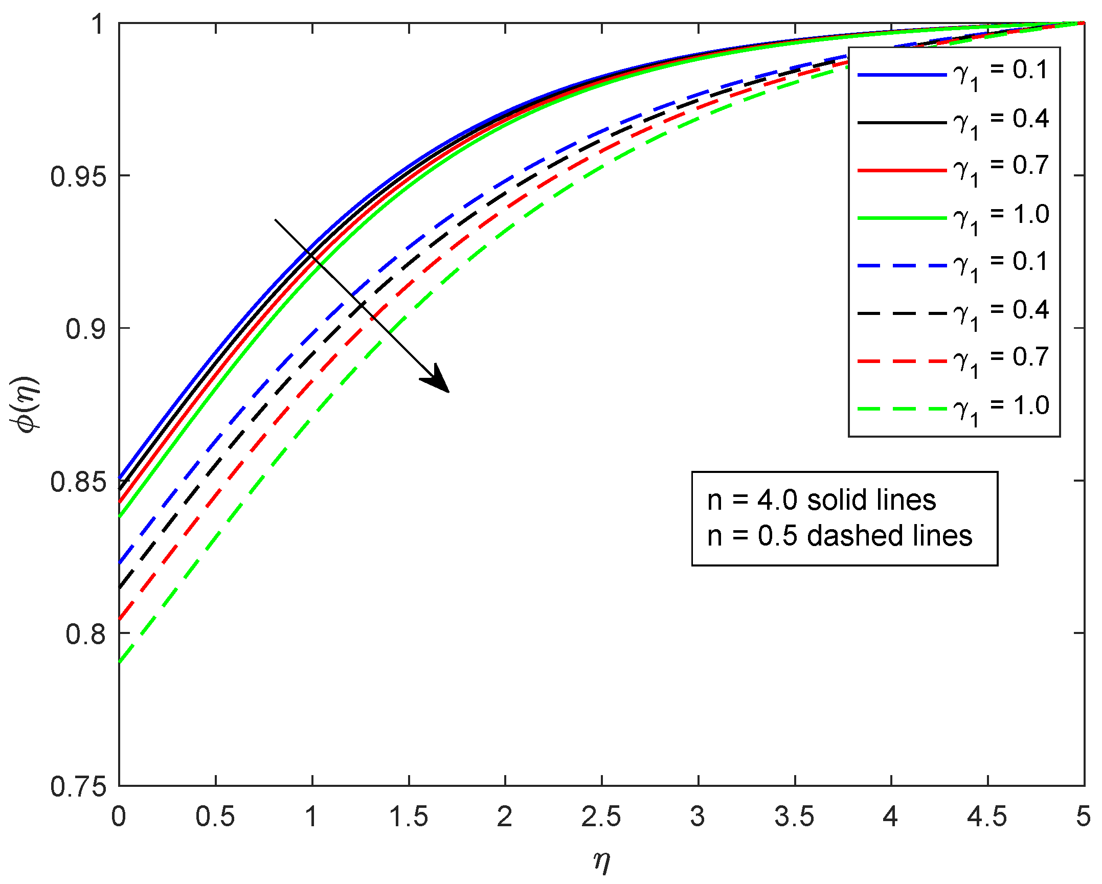
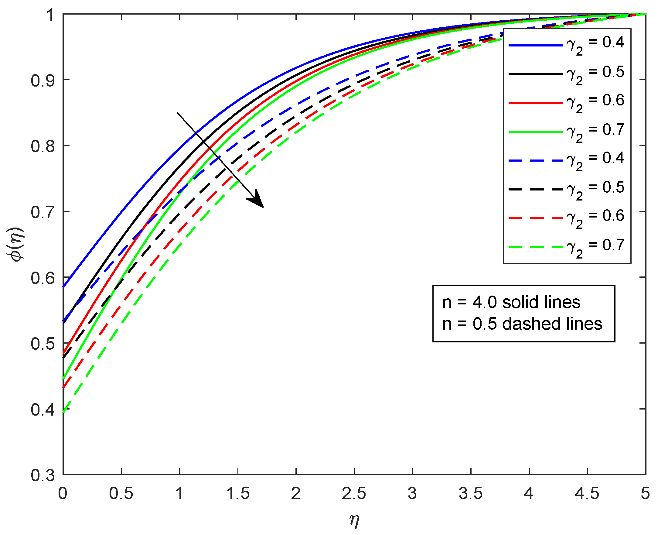
• Strength of homogeneous and heterogeneous reactions show the same decreasing trend on concentration distribution.
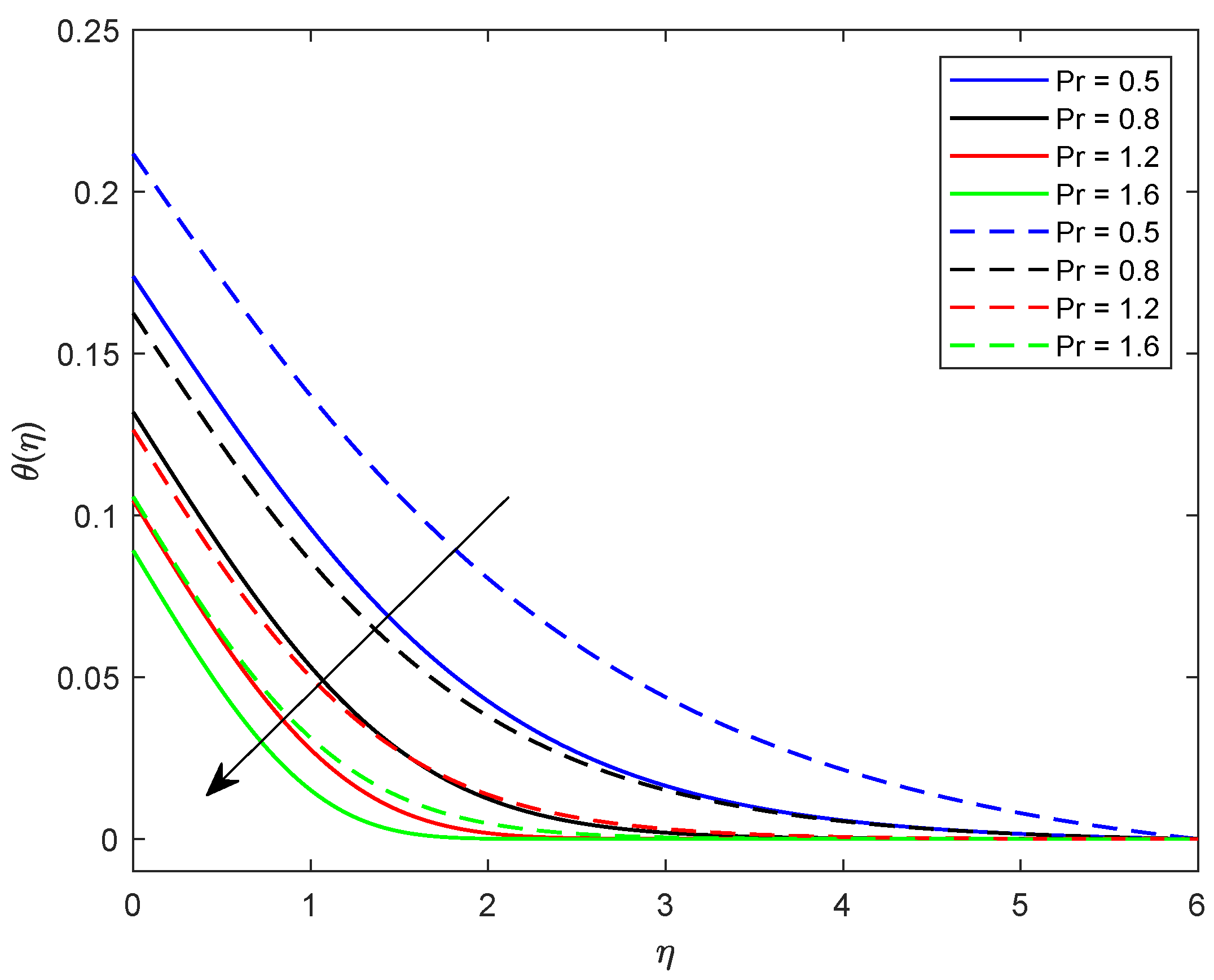
• Effects of Prandtl number and Biot number on temperature field are also conflicting.
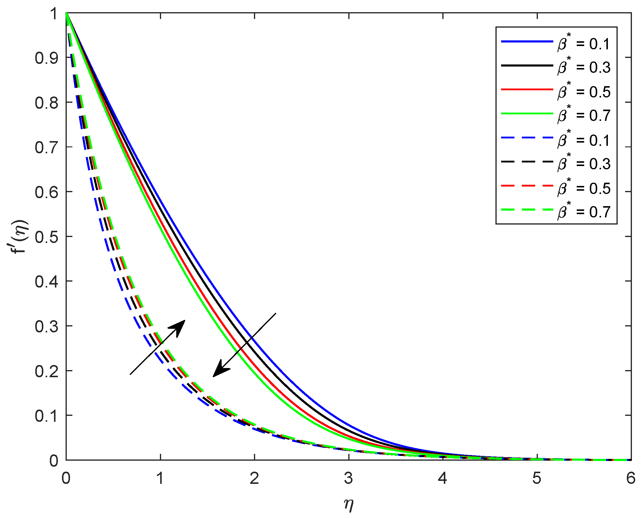
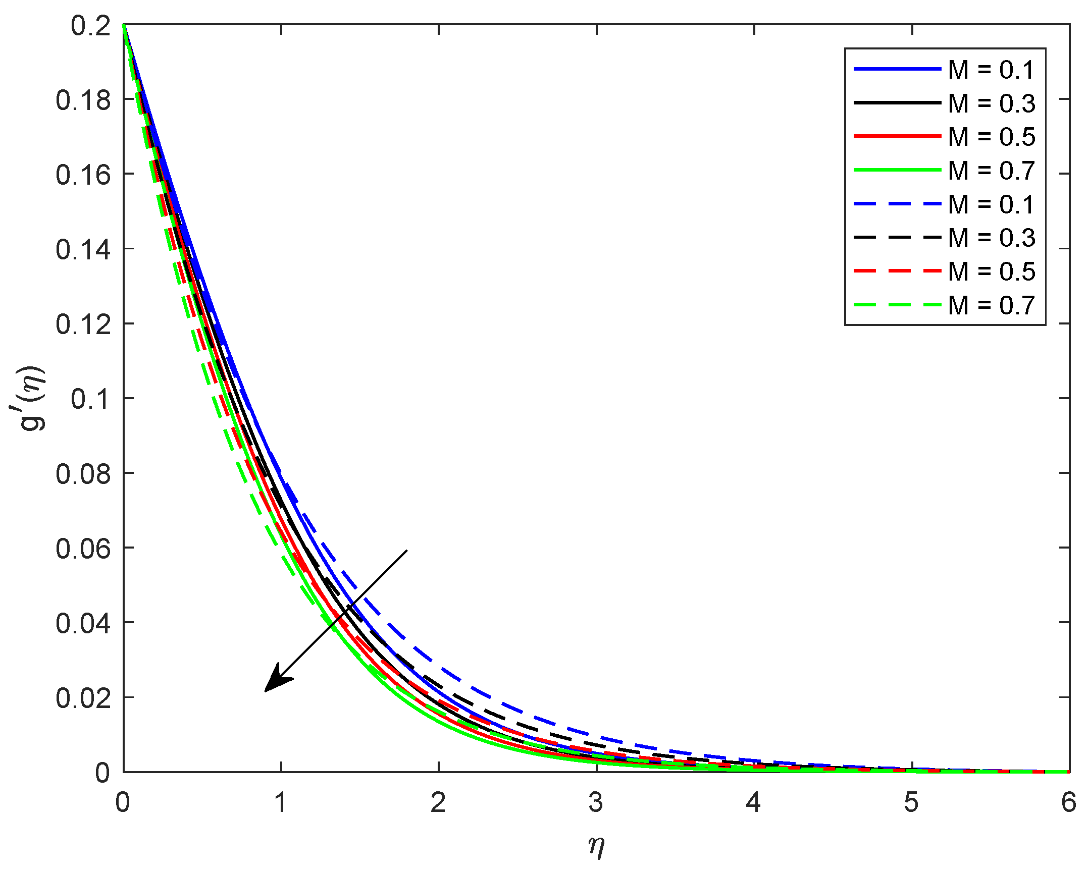
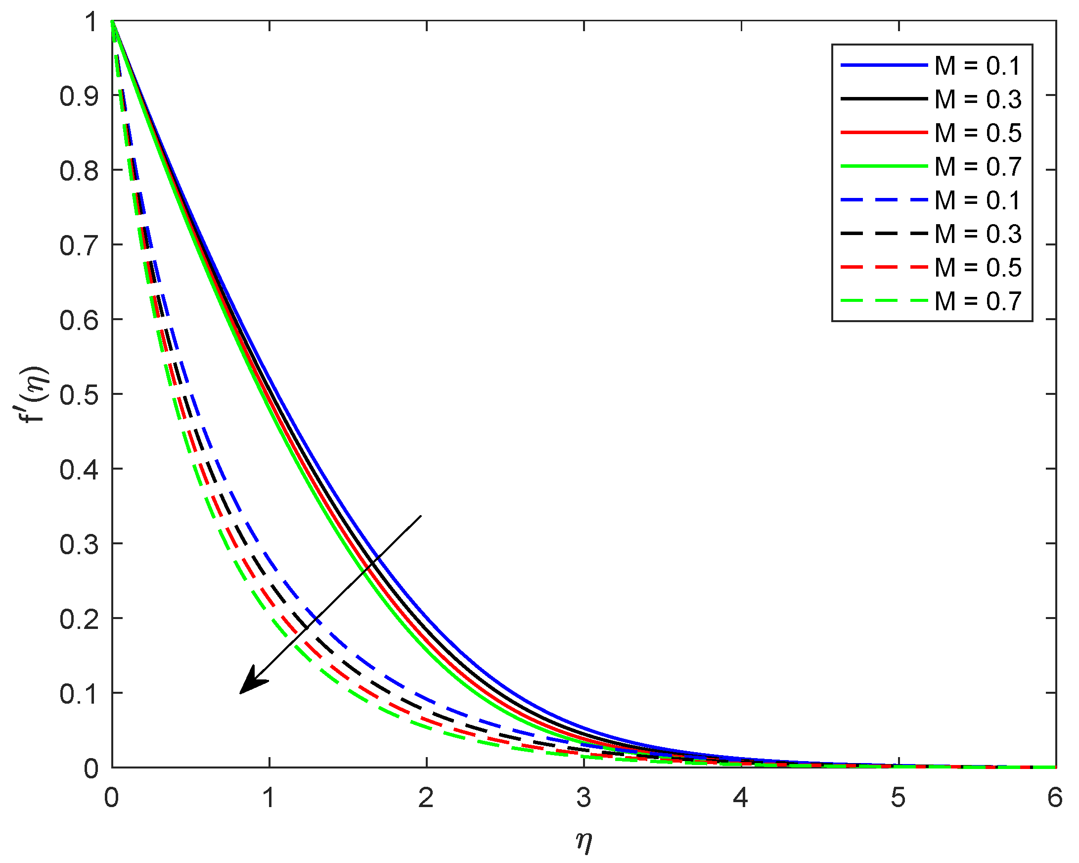
• The velocity of the fluid is in decline for a stronger magnetic effect.
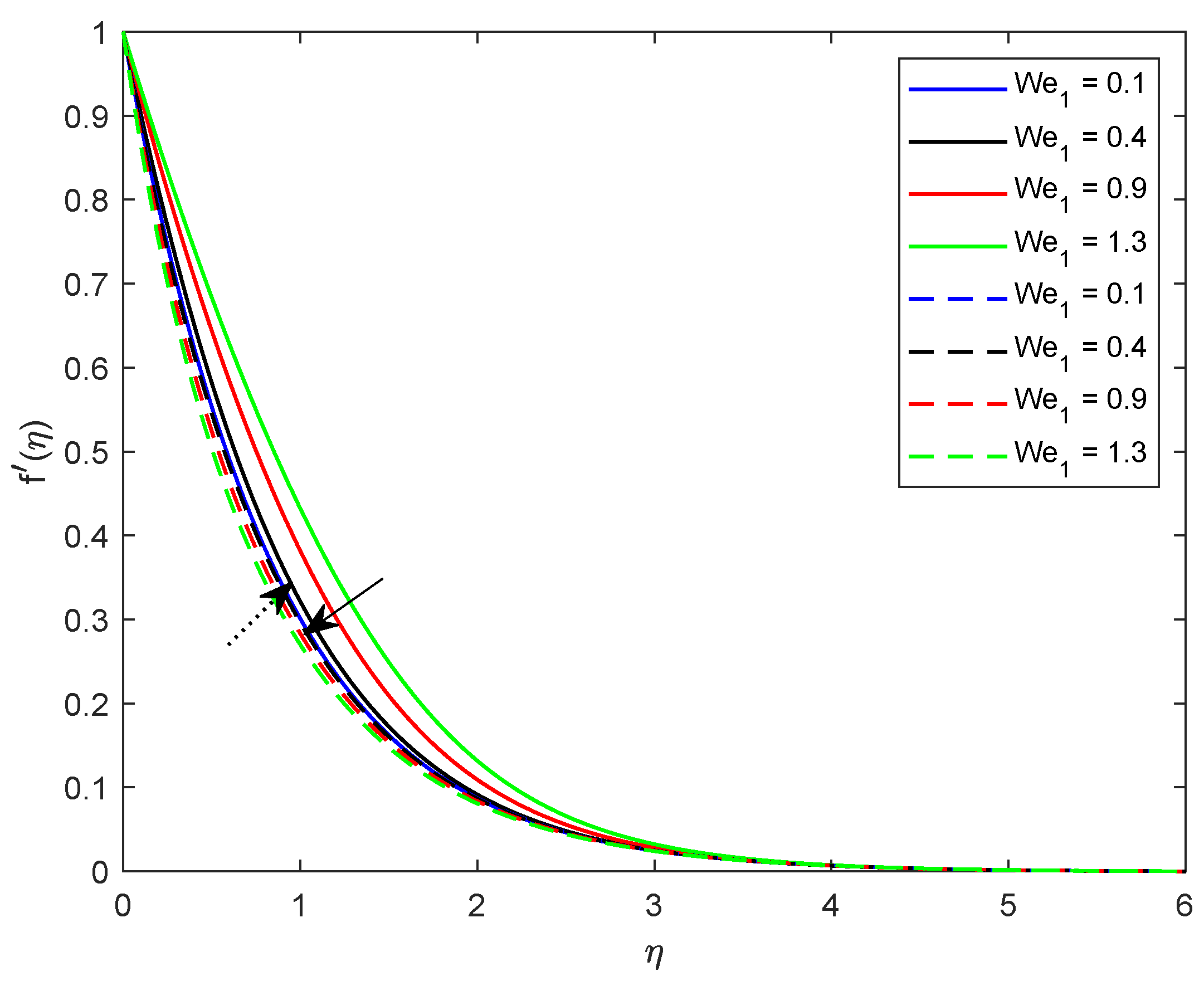
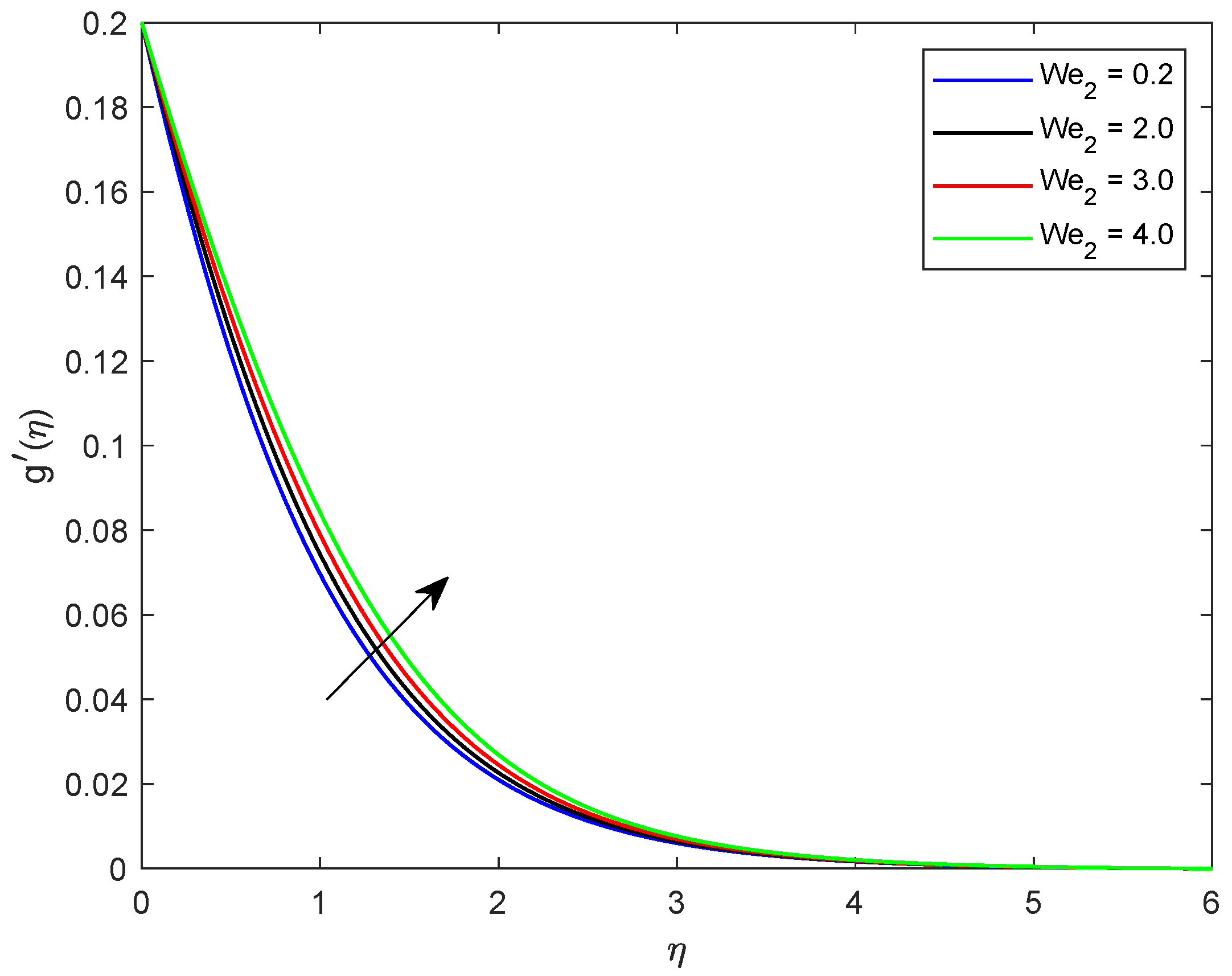
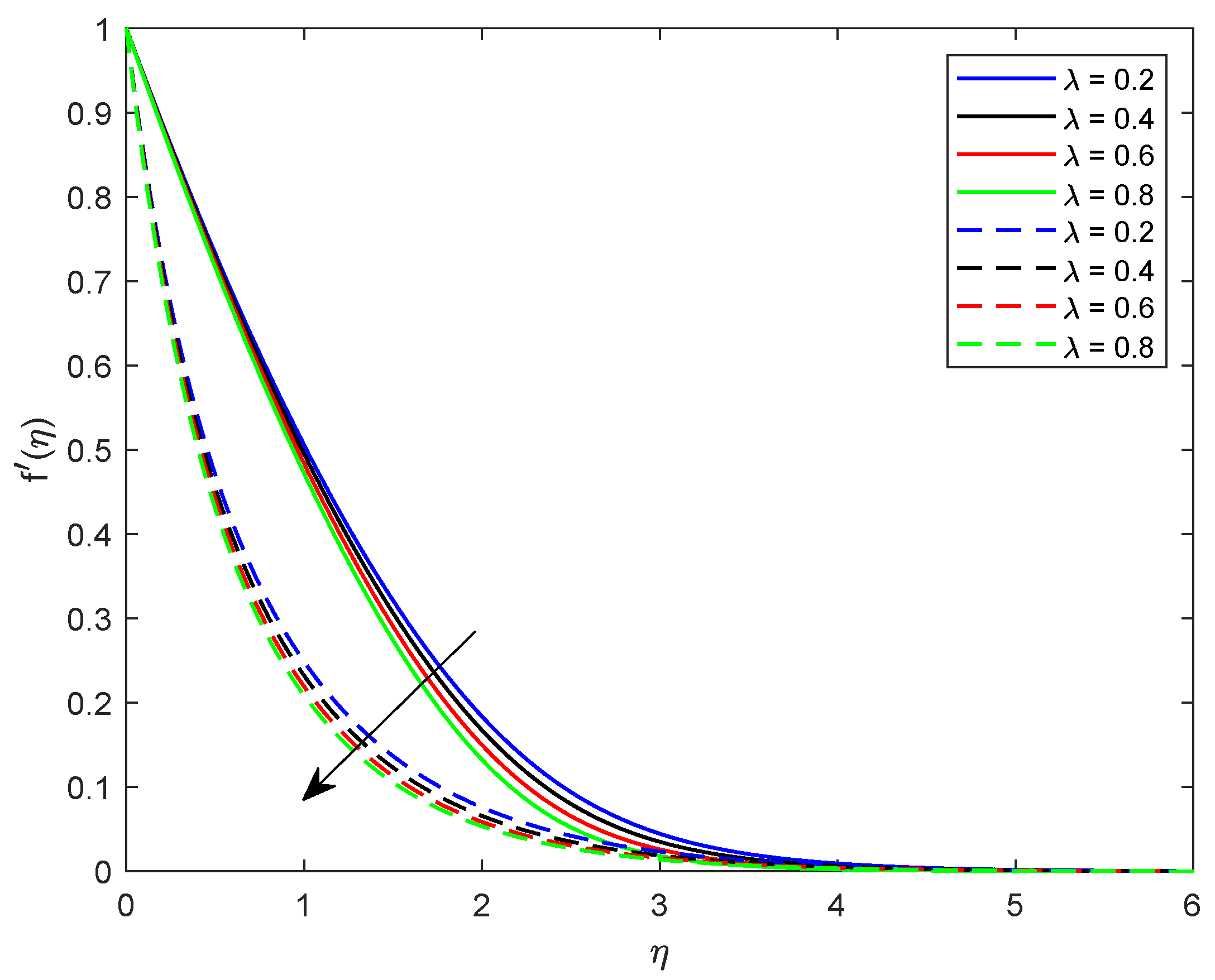
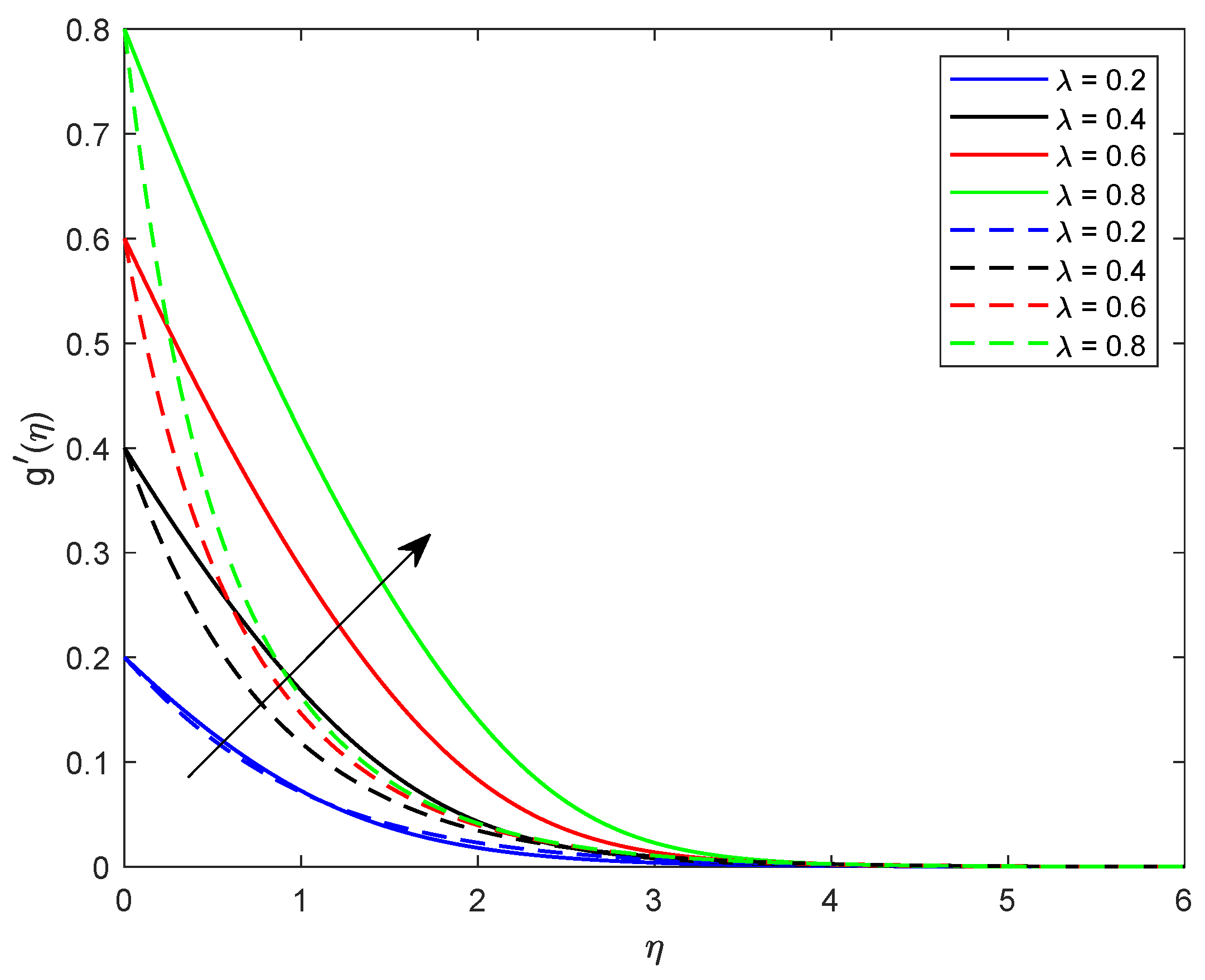
• Velocity escalates for growing estimates of ratios of stretching rate.
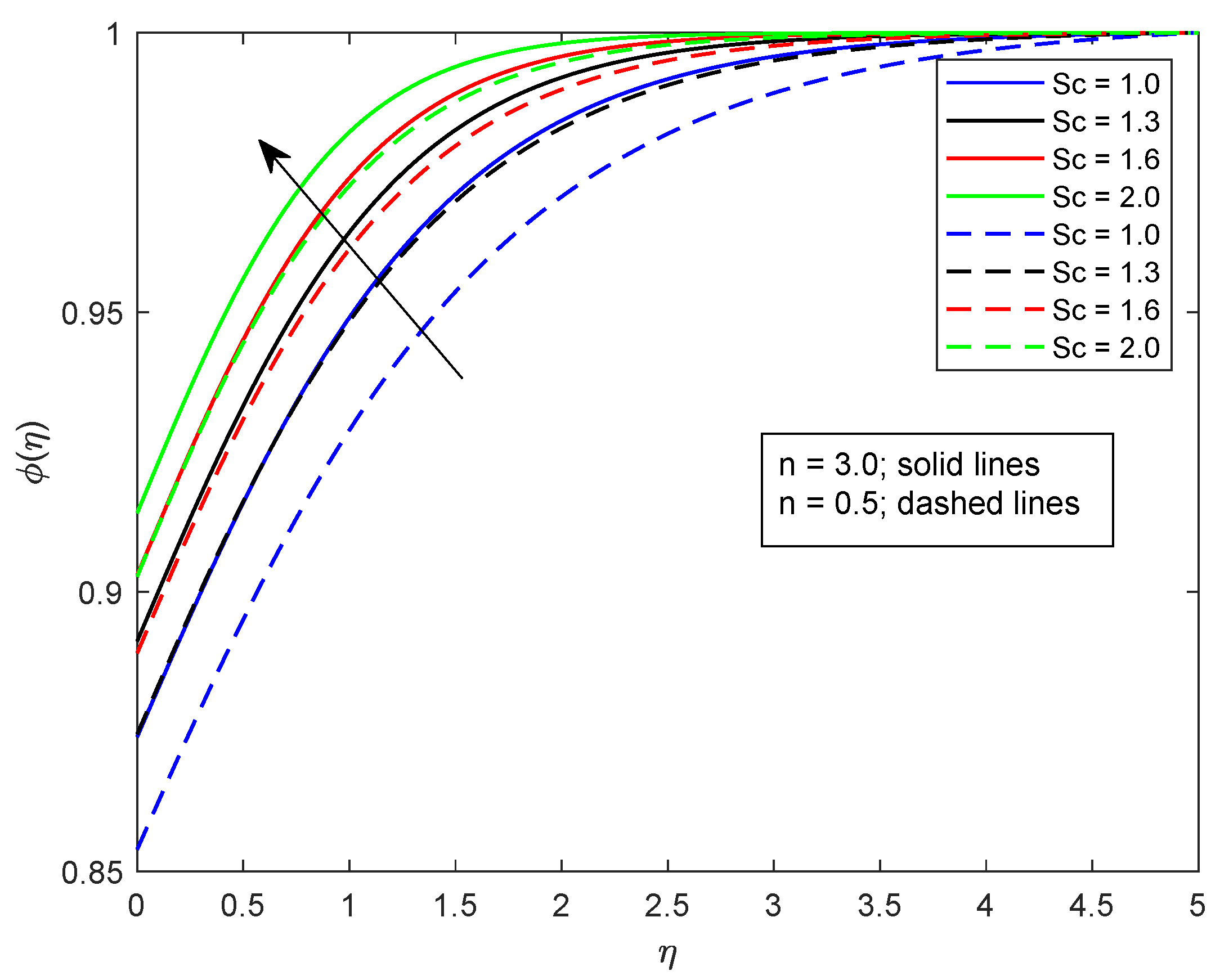
• With an increase in the value of the Schmidt number, the concentration of the fluid is enhanced.

References

1. Bird, R.; Byron, R.; Armstrong, R.C.; Hassager, O. Dynamics of Polymeric Liquids. Vol. 1: Fluid Mechanics; Wiley: London, UK, 1987. [Google Scholar]
2. Quoc, V.T.; Kim, B. Transport phenomena of water in molecular fluidic channels. Sci. Rep. 2016, 6, 33881. [Google Scholar]
3. Quoc, V.T.; Park, B.; Park, C.; Kim, B. Nano-scale liquid film sheared between strong wetting surfaces: Effects of interface region on the flow. J. Mech. Sci. Technol. 2015, 29, 1681–1688. [Google Scholar]
4. Ghorbanian, J.; Beskok, A. Scale effects in nanochannel liquid Flows. Microfluid. Nanofluid. 2016, 20, 121. [Google Scholar] [CrossRef]
5. Ghorbanian, J.; Celebi, A.T.; Beskok, A. A phenomenological continuum model for force-driven nano-channel liquid flows. J. Chem. Phys. 2016, 145, 184109. [Google Scholar] [CrossRef]
6. Carreau, P.J. Rheological equations from molecular network Theories. Trans. Soc. Rheol. 1972, 16, 99–127. [Google Scholar] [CrossRef]
7. Chhabra, R.P.; Uhlherr, P.H.T. Creeping motion of spheres through shear-thinning elastic fluids described by the Carreau viscosity equation. Rheol. Acta 1980, 19, 187–195. [Google Scholar] [CrossRef]
8. Bush, M.B.; Phan-Thien, N. Drag force on a sphere in creeping motion throug a Carreau model fluid. J. Non-Newton. Fluid Mech. 1984, 16, 303–313. [Google Scholar] [CrossRef]
9. Uddin, J.; Marston, J.O.; Thoroddsen, S.T. Squeeze flow of a Carreau fluid during sphere impact. Phys. Fluids 2012, 24, 073104. [Google Scholar] [CrossRef] [Green Version]
10. Tshehla, M.S. The flow of a Carreau fluid down an incline with a free surface. Int. J. Phys. Sci. 2011, 6, 3896–3910. [Google Scholar]
11. Khan, M.; Irfan, M.; Khan, W.A.; Alshomrani, A.S. A new modeling for 3D Carreau fluid flow considering nonlinear thermal radiation. Results Phys. 2017, 7, 2692–2704. [Google Scholar] [CrossRef]
12. Khan, M.; Ijaz, M.; Kumar, A.; Hayat, T.; Waqas, M.; Singh, R. Entropy generation in flow of Carreau nanofluid. J. Mol. Liq. 2019, 278, 677–687. [Google Scholar] [CrossRef]
13. Khan, M.; Irfan, M.; Khan, W.A. Thermophysical properties of unsteady 3D flow of magneto Carreau fluid in the presence of chemical species: A numerical approach. J. Braz. Soc. Mech. Sci. Eng. 2018, 40, 108. [Google Scholar] [CrossRef]
14. Irfan, M.; Khan, W.A.; Khan, M.; Gulzar, M. Influence of Arrhenius activation energy in chemically reactive radiative flow of 3D Carreau nanofluid with nonlinear mixed convection. J. Phys. Chem. Solids 2019, 125, 141–152. [Google Scholar] [CrossRef]
15. Vasu, B.; Ray, A.K. Numerical study of Carreau nanofluid flow past vertical plate with the Cattaneo–Christov heat flux model. Int. J. Numer. Methods Heat Fluid Flow 2019, 29, 702–723. [Google Scholar]
16. Waqas, M.; Farooq, M.; Khan, M.I.; Alsaedi, A.; Hayat, T.; Yasmeen, T. Magnetohydrodynamic (MHD) mixed convection flow of micropolar liquid due to nonlinear stretched sheet with convective condition. Int. J. Heat Mass Transf. 2016, 102, 766–772. [Google Scholar] [CrossRef]
17. Ramzan, M.; Farooq, M.; Hayat, T.; Chung, J.D. Radiative and Joule heating effects in the MHD flow of a micropolar fluid with partial slip and convective boundary condition. J. Mol. Liq. 2016, 221, 394–400. [Google Scholar] [CrossRef]
18. Besthapu, P.; Haq, R.U.; Bandari, S.; Al-Mdallal, Q.M. Mixed convection flow of thermally stratified MHD nanofluid over an exponentially stretching surface with viscous dissipation effect. J. Taiwan Inst. Chem. Eng. 2017, 71, 307–314. [Google Scholar] [CrossRef]
19. Khan, M.; Azam, M. Unsteady heat and mass transfer mechanisms in MHD Carreau nanofluid flow. J. Mol. Liq. 2017, 225, 554–562. [Google Scholar] [CrossRef]
20. Turkyilmazoglu, T. Mixed convection flow of magnetohydrodynamic micropolar fluid due to a porous heated/cooled deformable plate: Exact solutions. Int. J. Heat Mass Transf. 2017, 106, 127–134. [Google Scholar] [CrossRef]
21. Hayat, T.; Muhammad, T.; Shehzad, S.A.; Alsaedi, A. An analytical solution for magnetohydrodynamic Oldroyd-B nanofluid flow induced by a stretching sheet with heat generation/absorption. Int. J. Therm. Sci. 2017, 111, 274e288. [Google Scholar] [CrossRef]
22. Khan, M.I.; Waqas, M.; Hayat, T.; Alsaedi, A. A comparative study of Casson fluid with homogeneous-heterogeneous reactions. J. Colloid Interface Sci. 2017, 498, 85–90. [Google Scholar] [CrossRef]
23. Ramzan, M.; Bilal, M.; Chung, J.D. MHD stagnation point Cattaneo–Christov heat flux in Williamson fluid flow with homogeneous–heterogeneous reactions and convective boundary condition—A numerical approach. J. Mol. Liq. 2017, 225, 856–862. [Google Scholar] [CrossRef]
24. Ramzan, M.; Farooq, M.; Hayat, T.; Alsaedi, A.; Cao, J. MHD stagnation point flow by a permeable stretching cylinder with Soret-Dufour effects. J. Cent. South Univ. 2015, 22, 707–716. [Google Scholar] [CrossRef]
25. Su, X.; Zheng, L.; Zhang, X.; Zhang, J. MHD mixed convective heat transfer over a permeable stretching wedge with thermal radiation and ohmic heating. Chem. Eng. Sci. 2012, 78, 1–8. [Google Scholar] [CrossRef]
26. Pal, D.; Chatterjee, S. Soret and Dufour effects on MHD convective heat and mass transfer of a power-law fluid over an inclined plate with variable thermal conductivity in a porous medium. Appl. Math. Comput. 2013, 219, 7556–7574. [Google Scholar] [CrossRef]
27. Fourier, J.B.J. Théorie Analytique de la Chaleur; Chez Firmin Didot: Paris, France, 1822. [Google Scholar]
28. Cattaneo, C. Sulla conduzione del calore, Attidel Seminario Matematico e Fisico Dell. Modena Reggio Emilia 1948, 3, 83–101. [Google Scholar]
29. Christov, C.I. On frame indifferent formulation of the Maxwell–Cattaneo model of finite-speed heat conduction. Mech. Res. Commun. 2009, 36, 481–486. [Google Scholar] [CrossRef]
30. Ramzan, M.; Bilal, M.; Chung, J.D. Effects of MHD homogeneous-heterogeneous reactions on third grade fluid flow with Cattaneo–Christov heat flux. J. Mol. Liq. 2016, 223, 1284–1290. [Google Scholar] [CrossRef]
31. Hayat, T.; Khan, M.I.; Farooq, M.; Alsaedi, A.; Khan, M.I. Thermally stratified stretching flow with Cattaneo–Christov heat flux. Int. J. Heat Mass Transf. 2017, 106, 289–294. [Google Scholar] [CrossRef]
32. Sui, J.; Zheng, L.; Zhang, X. Boundary layer heat and mass transfer with Cattaneo–Christov double-diffusion in upper-convected Maxwell nanofluid past a stretching sheet with slip velocity. Int. J. Therm. Sci. 2016, 104, 461–468. [Google Scholar] [CrossRef]
33. Liu, L.; Zheng, L.; Liu, F.; Zhang, X. Heat conduction with fractional Cattaneo–Christov upper-convective derivative flux model. Int. J. Therm. Sci. 2017, 112, 421–426. [Google Scholar] [CrossRef]
34. Kumar, R.; Kumar, R.; Sheikholeslami, M.; Chamkha, A.J. Irreversibility analysis of the three-dimensional flow of carbon nanotubes due to nonlinear thermal radiation and quartic chemical reactions. J. Mol. Liq. 2019, 274, 379–392. [Google Scholar] [CrossRef]
35. Xu, H. Homogeneous–Heterogeneous Reactions of Blasius Flow in a Nanofluid. J. Heat Transf. 2019, 141, 024501. [Google Scholar] [CrossRef]
36. Sithole, H.; Mondal, H.; Magagula, V.M.; Sibanda, P.; Motsa, S. Bivariate Spectral Local Linearisation Method (BSLLM) for unsteady MHD Micropolar-nanofluids with Homogeneous–Heterogeneous chemical reactions over a stretching surface. Int. J. Appl. Comput. Math. 2019, 5, 12. [Google Scholar] [CrossRef]
37. Khan, W.A.; Ali, M.; Sultan, F.; Shahzad, M.; Khan, M.; Irfan, M. Numerical interpretation of autocatalysis chemical reaction for nonlinear radiative 3D flow of cross magnetofluid. Pramana 2019, 92, 16. [Google Scholar] [CrossRef]
38. Raees, A.; Wang, R.Z.; Xu, H. A homogeneous-heterogeneous model for mixed convection in gravity-driven film flow of nanofluids. Int. Commun. Heat Mass Transf. 2018, 95, 19–24. [Google Scholar] [CrossRef]
39. Lu, D.; Li, Z.; Ramzan, M.; Shafee, M.; Chung, J.D. Unsteady squeezing carbon nanotubes based nano-liquid flow with Cattaneo–Christov heat flux and homogeneous–heterogeneous reactions. Appl. Nanosci. 2019, 9, 169–178. [Google Scholar] [CrossRef]
40. Lu, D.; Ramzan, M.; Ahmad, S.; Chung, J.D.; Farooq, U. A numerical treatment of MHD radiative flow of Micropolar nanofluid with homogeneous-heterogeneous reactions past a nonlinear stretched surface. Sci. Rep. 2018, 8, 12431. [Google Scholar] [CrossRef]
41. Lu, D.; Ramzan, M.; Bilal, M.; Chung, J.D.; Farooq, U.; Tahir, S. On three-dimensional MHD Oldroyd-B fluid flow with nonlinear thermal radiation and homogeneous–heterogeneous reaction. J. Braz. Soc. Mech. Sci. Eng. 2018, 40, 387. [Google Scholar] [CrossRef]
42. Ramzan, M.; Bilal, M.; Chung, J.D. Influence of homogeneous-heterogeneous reactions on MHD 3D Maxwell fluid flow with Cattaneo–Christov heat flux and convective boundary condition. J. Mol. Liq. 2017, 230, 415–422. [Google Scholar] [CrossRef]
43. Nadeem, S.; Muhammad, N. Impact of stratification and Cattaneo–Christov heat flux in the flow saturated with porous medium. J. Mol. Liq. 2016, 224, 423–430. [Google Scholar] [CrossRef]
44. Hayat, T.; Rashid, M.; Alsaedi, A. Three dimensional radiative flow of magnetite-nanofluid with homogeneous-heterogeneous reactions. Results Phys. 2018, 8, 268–275. [Google Scholar] [CrossRef]
45. Merkin, J.H. A model for isothermal homogeneous–heterogeneous reactions in boundary layer flow. Math. Comput. Model. 1996, 24, 125–136. [Google Scholar] [CrossRef]
46. Chaudhary, M.A.; Merkin, J.H. A simple isothermal model for homogeneous-heterogeneous reactions in boundary layer flow: I. Equal diffusivities. Fluid Dyn. Res. 1995, 16, 311–333. [Google Scholar] [CrossRef]
47. Zargartalebi, H.; Ghalambaz, M.; Noghrehabadi, A.; Chamkha, A. Stagnation-point heat transfer of nanofluids toward stretching sheets with variable thermo-physical properties. Adv. Powder Technol. 2015, 26, 819–829. [Google Scholar] [CrossRef]
48. Ahmad, K.; Nazar, R. Magnetohydrodynamic three dimensional flow and heat transfer over a stretching surface in a viscoelastic fluid. J. Sci. Technol. 2010, 3, 1–14. [Google Scholar]
Figure 1. Geometry of the problem.
Symmetry 11 00618 g001
Figure 2. Illustration of W e 1 versus f ( η ) .
Symmetry 11 00618 g002
Figure 3. Illustration of W e 2 versus g ( η ) .
Symmetry 11 00618 g003
Figure 4. Illustration of β * versus f ( η ) .
Symmetry 11 00618 g004
Figure 5. Illustration of M versus g ( η ) .
Symmetry 11 00618 g005
Figure 6. Illustration of M versus f ( η ) .
Symmetry 11 00618 g006
Figure 7. Illustration of λ versus f ( η ) .
Symmetry 11 00618 g007
Figure 8. Influence of λ on g ( η ) .
Symmetry 11 00618 g008
Figure 9. Illustration of P r versus θ ( η ) .
Symmetry 11 00618 g009
Figure 10. Illustration of ϵ versus θ ( η ) .
Symmetry 11 00618 g010
Figure 11. Illustration of S c versus ϕ ( η ) .
Symmetry 11 00618 g011
Figure 12. Illustration of λ 1 versus θ ( η ) .
Symmetry 11 00618 g012
Figure 13. Illustration of δ versus θ ( η ) .
Symmetry 11 00618 g013
Figure 14. Illustration of γ 1 versus ϕ ( η ) .
Symmetry 11 00618 g014
Figure 15. Illustration of γ 2 versus ϕ ( η ) .
Symmetry 11 00618 g015