An Iterated Hybrid Local Search Algorithm for Pick-and-Place Sequence Optimization


1
School of Mechanical, Electronic and Control Engineering, Beijing Jiaotong University, Beijing 100044, China
2
School of Economics and Management, Beijing Jiaotong University, Beijing 100044, China
*
Author to whom correspondence should be addressed.
Symmetry 2018, 10(11), 633; https://doi.org/10.3390/sym10110633
Submission received: 14 October 2018
/
Revised: 6 November 2018
/
Accepted: 9 November 2018
/
Published: 13 November 2018
(This article belongs to the Special Issue Symmetry in Computing Theory and Application)
Abstract
:This paper shows the results of our study on the pick-and-place optimization problem. To solve this problem efficiently, an iterated hybrid local search algorithm (IHLS) which combines local search with integer programming is proposed. In the section of local search, the greedy algorithm with distance weight strategy and the convex-hull strategy is developed to determine the pick-and-place sequence; in the section of integer programming, an integer programming model is built to complete the feeder assignment problem. The experimental results show that the IHLS algorithm we proposed has high computational efficiency. Furthermore, compared with the genetic algorithm and the memetic algorithm, the IHLS is less time-consuming and more suitable in solving a large-scale problem.
1. Introduction
The Printed Circuit Board (PCB) is a vital part of electronic products such as smart phones, laptops, and monitors. It contains large amount of components and becomes more and more complicated. In a typical surface mount technology assembly line, PCBs go through a series of processes: solder or adhesive application; component pick-and-place; reflowing; cleaning; testing; and inspection [1]. The pick-and-place process is the most time-consuming procedure. In order to improve production efficiency economically, the pick-and-place sequence optimization is an economical way to reduce production times, and it is the key point to improve production efficiency.
In previous researches, pick-and-place sequence optimization problem has drawn great attentions. There are three sub-problems to be considered in pick-and-place problems: place sequence, feeder assignment and nozzle assignment [2]. Basically, the place sequence (see Section 2.1 steps (2) and (5)) can be considered as the Traveling salesman problem (TSP) or the Vehicle routing problems (VRP) [3,4]. The feeder assignment (see Section 2.1 step (6)) can be viewed as the assignment problem [5]. As to the nozzle assignment, the problem is that different components are assigned to corresponding nozzles, and the object is to minimize the number of nozzle changes. Some researchers do not take the nozzle assignment into consideration in some cases [6,7].
Because of the complexity of the problem, heuristic approaches, such as meta-heuristic approaches and multi-stage heuristics strategy are widely used, while several exact methods can be found in previous research. Meta-heuristic approaches such as genetic algorithm (GA), simulated annealing (SA), particle swarm optimization (PSO) and ant colony optimization (ACO), which play an important role in solving complex problems [8,9,10,11,12], are altered to adapt to solving the problem efficiently [13,14,15,16]. Zhu and Zhang [17] added self-variation behavior to the frog leaping algorithm, which has good accuracy. Multi-stage heuristics strategy, combines the advantages of several algorithm strategies with good performance. Lin and Huang [18] aimed at minimizing total PCB assembly time, and proposed a hybrid genetic algorithm combined with the nearest neighbor search, 2-optimization and genetic algorithm to obtain the optimal component pick-and-place sequence. Similarly, a new mechanism to minimize the assembly time for a multi-headed gantry and high-speed surface mounting technology machine by determining the component assignment to feeder slots was proposed by Han and Seo [19]. The presenting of the heuristic is based on the feeder assignment, which consists of nearest component allocation and globally updated assignment. This algorithm leads to better performance than genetic algorithm or 2-opt swap search. Luo and Liu [20] proposed a two-stage mixed-integer linear programming model and a two-stage problem-solving frame with a hybrid evolutionary algorithm (HEA). The constructive two-stage heuristics is not only determine the set of nozzle types assigned to each head and the total number of assembly cycles, but solve all the sub-problem respectively. As for exact methods, the conventional method is integer programming, and the main measure is modeling and improvement of integer programming model. In research of integer programming models, several researchers focus on the total traveling distance, while others aim at minimizing the assembly completion time. Kumar and Li [21] developed a technique based on integer programming to determine an optimal assignment of feeders as well as an optimal sequence of pickup and placements, furthermore, they obtained optimal solutions based on minimum weight matching and traveling salesman problem. Altinkemer and Kazaz et al. [22] applied an integrated approach which tackles each sub-problems as a single problem simultaneously, and they also presented an -approximation algorithm with an -error gap for the PCB problem. Ho and Ji [23] formulated several mathematical models for determining the optimal sequence of component placements and the assignment of component types to feeders simultaneously, or for determining the integrated scheduling problem for the sequential pick-and-place machine. The objective of integrated problem is to minimize the total distance traveled by the placement head. Luo and Liu [24] formulated the scheduling optimization problem as a mixed integer linear programming model. And the model was applied to the assembly sequence of placement locations and the assignment of pick-and-place heads for locations so as to minimize the assembly time.
The former researchers widely used effective approaches, such as integer programming, meta-heuristic approaches and hybrid heuristics, to obtain a best solution of pick-and-place sequence optimization problem. These approaches are mainly focused on the optimality of the algorithm results, but paid less attention on time consumption of the algorithm in solving large-scale problems. The aim of present work is to establish an effective multi-stage method with less time-consuming and obtain the optimal solution of the large-scale problem. Considering these restrictions, we propose an integrated hybrid local search (IHLS) algorithm which can meet the time requirements of actual production. Differ from conventional approach which is population based bionic algorithm, the proposed IHLS is a two-stage algorithm which combines the local search method with integer programming method. The main contributions of this paper are: (1) the convex-hull based adjustment strategy is developed to adjust the sequence; (2) a simplified integer programming model of feeder assignment is developed and integrated in the algorithm.
The rest of this paper is organized as follows. In Section 2, the machine structure and PCB assembly process are described, and a simplified mathematical model is proposed. Section 3 is devoted to the description of the IHLS algorithm which combines integer programming with local search. Computational experiments are described in Section 4, which verifies that the algorithm we proposed is superior to genetic algorithm and memetic algorithm in large-scale problems. Finally, conclusions are drawn in Section 5.
2. The Description of Pick-and-Place Sequence Optimization Problem
In this section, the basic structure of pick-and-place machine is described in sufficient detail, and then the PCB assembly processes are introduced. The following description is demonstrating the simplified pick-and-place optimization problem.
2.1. Machine Structure and PCB Assembly Process
As shown in Figure 1 PART I, the main structure of the placement machine is composed of the body frame for fixing other structures, the PCB conveyor for transmitting the PCB, the workbench for fixing and supporting the PCB, the mounting head with a moveable arm for mounting components in x and y directions, and several feeder slots for laying different type of components feeders. As for PCB, as shows in Figure 1 PART III, there is a large amount of points on PCB and each point needs to be mounted with an electrical component. As for feeder, it is a depot for electric components and each feeder only contains one type of electric components.
The assembling process of the PCB by the machine mainly involves the following steps.
- (1)
- The PCB is transmitted to the workbench by PCB conveyor.
- (2)
- The PCB is fixed on the workbench, and the coordinates of points on PCB (see Figure 1 PART III) are loaded in the work coordinate system.
- (3)
- The mounting head moves to the corresponding feeder slots according to a sequence. There are several nozzles on the mounting head, and each nozzle can only grip one component. Thus, the maximum number of components to be carried by the head is the nozzle number (see Figure 1 PART II).
- (4)
- In order to identify the type of components carried by each nozzle, the mounting head should be scanned by camera before moving to workbench, so as to find the corresponding position on PCB.
- (5)
- All the components carried by the mounting head are mounted onto PCB.
- (6)
- The mounting head after mounted moves to the corresponding feeders which are assigned feeder slots, then the head repeat step (3) to step (5) until all the points on PCB are finished. Then, PCB conveyor starts loading the next PCB.
Step (1) and step (2) are the preparing stage in PCB assembly process. Step (3) to step (5) can be defined as a pick-and-place cycle which is the key point of pick-and-place optimization problem. In order to simplify the problem, step (4) is usually ignored in the research. In general, the number of pick-and-place cycles mainly depends on the point number and the nozzle number. The next section will illustrate the simplified problem and notifications.
2.2. The Problem Simplification and Notifications
Step (1) to step (6) are PCB assembly process in real production environment. In researches, the pick-and-place sequence optimization problem is usually simplified while solving the problem. The simplification mainly involves following essential parts.
- (1)
- Each feeder only contains one component type and can only be assigned to one feeder slot.
- (2)
- Each point on PCB needs one component and is only allowed to mount once.
- (3)
- The mounting head needs to pick up components among feeders first, and then the head moves to corresponding points on PCB without scanning procedure by camera.
In addition, the problem assumes that all the nozzles on the head can grip all types of components. Therefore, the exchange of nozzles is not considered in this paper. To better demonstrate the problem, the notifications used in the model are explained as follows.
Parameters:
| The total points’ position in x direction on PCB | |
| The total points’ position in y direction on PCB | |
| The total points need component type on PCB | |
| The total number of points on PCB | |
| The number of nozzles | |
| The total number of feeder slots | |
| The total number of component types | |
| The total number of pick-and-place cycles, | |
| The first feeder slot position in x direction | |
| The first feeder slot position in y direction | |
| The fixed distance between adjacent feeder slots, because all the feeder slots have the same coordinate in y direction, the distance is the difference between two adjacent coordinates in x direction actually | |
| The Euclidean distance between point and point on PCB | |
| The Euclidean distance between point and feeder slot | |
| The number of points to be mounted in kth pick-and-place cycle, , where ; , where |
The distance between points on PCB can be calculated by formula (1).
The distance between point and feeder slot can be calculated by formula (2).
Variables:
| is the pick-and-place sequence in kth pick-and-place cycle, | |
| Whether the component type is assigned to the feeder slot , if is assigned to slot , ; otherwise, . , . |
2.3. Mathematical Model of the Problem
The aim of this paper is to minimize the total movement distance of mounting head. The object function of the mathematical model of pick-and-place problem is mainly divided into three parts. The first part is component placement distance on PCB, ; the second part is the component pick up distance among feeders, ; the third part is the movement distance of mounting head between points on PCB and feeders in feeders slots, .
The object function of the model can be described by formulas (3)–(10).
Subject to
where, formula (7) assures that each feeder slot can be assigned to one type of component feeder at most. Formula (8) assures that each type of component feeder must be assigned to one feeder slot. Formula (9) assures that all the component feeders must be assigned. Formula (10) assures that all the points on PCB must be mounted.
The value of depends on the place sequence , and the value of and also depend on variable . Similarly, affects the place sequence , which is . The model of this problem is complicated, which has motivated a lot of researchers to develop kinds of approaches to solve this problem. Generally, it is difficult to solve the problem in an integrated method. Therefore, we propose an algorithm which solves the model in two-stage. The first stage is obtaining the pick-and-place sequence while the value of is minimum. The second stage is obtaining the feeder assignment while the value of is minimum.
3. Iterated Hybrid Local Search Algorithm
The iterated hybrid local search algorithm, a two-stage based algorithm, mainly consists of local search and integer programming method. In the first stage, the local search method obtains the pick-and-place sequence while the value of is minimum. Based on the obtained , in the second stage, the integer programming aims at obtaining the value of while the value of is minimum. The measures of the local search include greedy strategy with distance weight, adjustment strategy based on convex-hull, termination criteria, and the feeder assignment problem based on the integer programming method. The details of these parts will be explained in the following section. In the algorithm, there are several parameters adopted, and they are explained below.
| The solution of pick-and-place distance in each interaction. | |
| The best solution of pick-and-place total distance in iterations. | |
| The best solution of pick-and-place sequence in iterations. | |
| The best object function value of feeder assignment model in iterations. | |
| The best solution of feeder assignment in iterations. | |
| The distance weight which is proposed based on splitting unit circle. is used to generate initial pick-and-place sequences and it can be obtained by formula (13). |
As shown in Figure 2, a circle with a radius of 1 () is divided into H parts, the circumference of circle is , therefore the arc length of each part is . Similarly, the angle of each part is , the angle between point i and 1 is which equals to . The distance from point to point 1 is in the circle. The relationship between the distance and can be expressed as an equation, . The distance can be determined. Therefore, , the ratio which equals to the distance between the point and point divide by the sum distance, including the distance between point and point 1 as well as the distance between point and point , in a unit circle. For example in Figure 2, the angle between point 3 and point 1 is , the relationship equation is , the distance from point 3 to point 1 is , while , then .
where, is the index of nozzles in mounting head.
3.1. The Greedy Strategy with Distance Weight
The pick-and-place sequence initialization is aimed at obtaining initial sequences which have better qualities. During the iterations of heuristic method, obtaining a better feasible solution contributes to the improvement of efficiency at the beginning. In this section, we propose a greedy strategy with distance weight to initialize the sequences.
After determining , the weighted distance can be represented as formula (14), if point as the ith sequence in .
where is the value of weighted distance, represents the point which is not allocated to , and represents the ith sequence in .
Formula (15) represents that the ith sequence in is the encoding of the point which has a minimum value of . The pick-and-place sequence initial pseudo code is given below.
- Step 1:
- Start calculate kth pick-and-place cycle where .
- Step 2:
- If the first iteration involves this process, and is other random encoding of points; else, (See Section 3.4) and is other random encoding of points.
- Step 3:
- In kth pick-and-place cycle, as is confirmed, calculate each by formula (14) and let while the corresponding satisfies , from to .
- Step 4:
- If , output the initial sequence ; otherwise, and repeat from step 3 to step 4.
For example, the total number of points on PCB is 6, the coordinates of points are shown in Table 1. The number of nozzles is 6, the pick-and-place sequence cycle number is 1, as shown in Figure 2. In order to initialize , can be determined, which are , , , , . As , the next sequence need to be determined based on the values of , , , and . The values of above items are , , , and . According to formula (15), , which is the minimun among . The next squence depends on the value of , , and . In this way, the sequence of can be determined. This strategy is aimed at initializing the sequence so that it is a better feasible solution, but the length of each sequence is not the minimum. So the adjusting strategy is needed to get a sequence of minimum distance.
3.2. The Adjusting Strategy Based on Convex-Hull
To adjust the sequence, each initial pick-and-place sequence can be regarded as a small size traveling salesman problem (TSP). For the traveling salesman problem, there are several classifications and extensions, such as symmetric traveling salesman problem (STSP), asymmetric traveling salesman problem (ATSP) and multiple traveling salesman problem (MTSP). Laszlo Barna Iantovics [25] proposed a novel universal metric and solved STSP by intelligent cooperative multi-agent systems. Furqan Hussain Essani [26] presented an algorithm combined colored petri nets and guaranteed a feasible solution to the MTSP with asymmetric cost matrix. Differ from above methods, the TSP in this section needs several simple measures to guarantee the efficiency of the algorithm and obtain a better feasible solution. Based on convex-hull algorithms [27], an approximate method is developed, and the details are explained below.
where represents the additional length, if line is replaced by line and line .
The pick-and-place sequence adjustment pseudo code of each cycle is given below.
- Step 1:
- Let , .
- Step 2:
- Select each item from , ; Select each pair of items from , . Calculate the value of .
- Step 3:
- Find the corresponding , where satisfies ; put into between and , remove from .
- Step 4:
- If , turn to step 7; otherwise, repeat from step 2 to step 3.
- Step 5:
- Update , let .
For example, as shown in Figure 3, , and . The dashed lines represent the additional length when the point is added to , the solid lines represent the length between two adjacent points in sequence. Each additional length of item in () and line 2–6 in () can be obtained, which are , and . The smallest value of is , and then , .
During the sequence adjustment, the additional length of each adjusting measure (step 3) is considered, and only the adjustment of minimum length will be accepted in this strategy. In other words, all cases of adjustment can be accepted based on formula (16). Therefore, the length of initial is minimum after the adjusting strategy.
3.3. Feeder Slots Selection
The feeder slots selection is based on the pick-and-place sequence . In order to improve efficiency, a new feeder assignment integer programming model is built in this section, and the model is solved by integer programming method. This model is modified based on the mathematical model (Section 2), replaced several variables, and retained the original constraints. As is determined, we generate parameters and .
| The number of links between component type and , where and . | |
| The first or last point in each pick-and-place cycle , where . |
Because is the encoding of points, represents the corresponding component type of . As is known, the corresponding component types of are , which . In the component type vector , is a link between component type and . The parameter is the total number of links between component type and , and it can be obtained by result . Initialize , then can be obtained from as formula (17).
For example, the component type vector is , the corresponding links can be obtained as following Table 2.
As for , formula (18) demonstrates the relationship between and .
In the second stage, the object function should be (formulas (5) and (6) in Section 2.1). It can be expressed as . represents the corresponding component type, when is obtained in first stage. Based on above works, replaces , and replaces . Without modifying of constraints, the new local integer programming model is described as follows:
Subject to
Binary variable represents whether the ith component type feeder is in the slot , and represents the corresponding sequence of th component type. Therefore, indicates the number of feeders between slot and . While demonstrates the total distance of the mounting head movements among feeders, it is the same as in Section 2.3. is encoded of first or last point in each sequence, while is the distance between the point and feeder slot . Therefore, represents the distance between point and the corresponding feeder type slot. demonstrates the total moving distance of mounting head between points on PCB and feeders in slots, which is the same as in Section 2.3.
The object function is to minimize the total distance of mounting head based on the pick-and-place sequence . And the constraints of this model are as same as the model in Section 2.3.
3.4. Initialization Update and Termination Criteria
In this algorithm, we obtain a feasible solution including pick-and-place sequence and feeder assignment . To improve the quality of solution, selecting based on the maximum length and resetting sequence are crucial iteration strategy. During each iteration, needs to be recorded if the value of the length is maximum, and this sequence needs to be reset first in next iteration, which is (see Section 3.1). can be generated by formula (20).
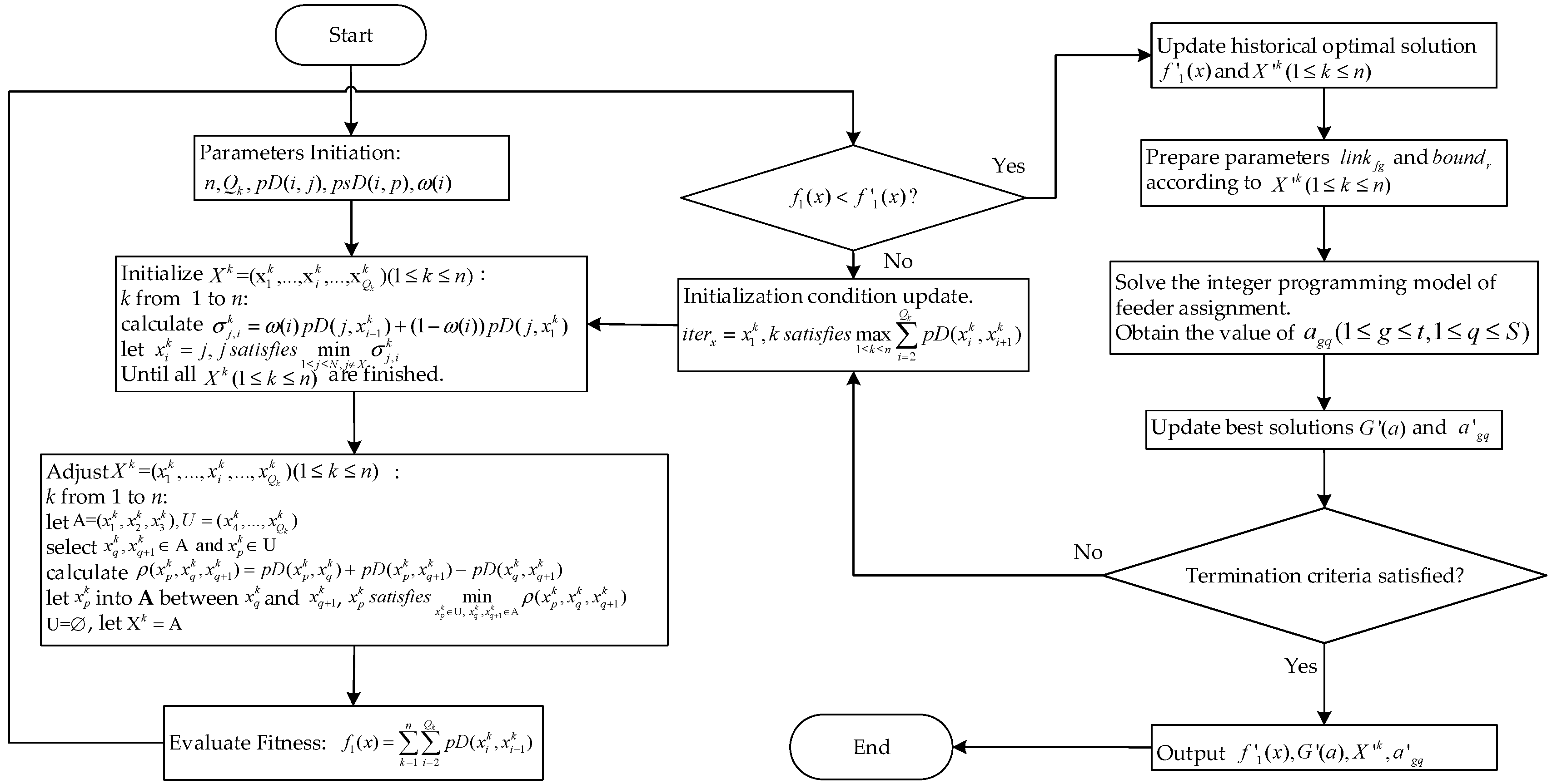
The IHLS algorithm is terminated when the number of iterations equals to the maximum number of iterations. The flowchart of the IHLS (Figure 4) and pseudo code are given below.
- Step 1:
- Initialize the parameters.
- Step 2:
- Initialize the pick-and-place sequence with according to greedy strategy, where .
- Step 3:
- Adjust the pick-and-place sequence by adjustment strategy, where .
- Step 4:
- Calculate the fitness value .
- Step 5:
- If the best solution , turn to step 6; otherwise, repeat from step 3 to step 5.
- Step 6:
- Update the record best solution , let and .
- Step 7:
- According to , relevant parameters ( and ) are prepared and input to feeder assignment model.
- Step 8:
- Update the best solutions and , let and .
- Step 9:
- If termination criteria was satisfied, turn to step 10; otherwise, repeat from step 3 to step 8.
- Step 10:
- Output the best solutions.
4. Experimental Results and Analysis
In order to verify the effectiveness of IHLS algorithm, three other test algorithms are selected for comparison. The three baseline algorithms are genetic algorithm (GA), memetic algorithm and integer programming method. The algorithms are implemented in MATLAB and run with the 2.8 GHz computer with 16 GB RAM. The integer programming models are solved by Yalmip with Cplex1263.
4.1. Comparison with Exact Algorithm
As for integer programming, because integer programming method can only solve very small-scale problems, the place sequence integer programming model and several small instances except instance 4 are generated based on the research of Ho and Ji [2].
The IHLS is executed on very small-scale instances and the results are obtained by integer programming method, Cplex. Three small-scale instances with 6 feeder slots are given in Table 3. The results show that IHLS is near to the optima as the average gap is 6.29%. While the instance 4 (the nozzle number of instance 4 is 1) shows that the integer programming method cannot solve the problem with a larger scale.
4.2. Comparison of the Heuristics in Different Size Instances and Analysis
In this experiment, the performance of the algorithm is tested on 9 PCB instances. These 9 PCB instances are generated based on industrial data.
(1) Set the model parameters
The model parameters, such as , , , , and , are based on the test instances, and other parameters, such as , , , , and , are based the pick-and-place machine parameters. The parameters are introduced in Table 4.
The total number of components () ranges from 82 to 300 and the component type (t) ranges from 3 to 9. The solving complexity of instances mainly depend on the number of components. With the increasing of , the difference between algorithms performance can be more and more significant.
(2) Comparison with the heuristics
In the GA algorithm, the chromosome structure is decimal code, and each chromosome includes PCB placement sequence part and feeder assignment part. The chromosome structure can be found in Kulak, Yilmaz and Günther [13]. The population size is 2000, the crossover rate is 90%, and the mutation rate is 10%. As for memetic algorithm, based on Carlos’ research [28], the memetic algorithm used GA frame in population-based search, and the greedy strategy is used in local search part. The parameters of the memetic algorithm are the same as GA’s. The three algorithms, IHLS, GA and memetic algorithm, solve these instances based on the mathematical model in Section 2. The optimization results of each instance are the average values of 5 independent runs. The solutions are presented in Table 5. , and represent the total distance of GA, IHLS and memetic algorithm respectively. , and represent the CPU times of each algorithm.
(3) Experimental results analysis
There are different iteration strategies in three algorithms. The three algorithms obtain the optimal solution when the iteration achieves the maximum iteration number. But the solutions are different among the three algorithms. As shown in the second, forth, sixth and eighth column in Table 5, from instance 1 to instance 4 except instance 2, the minimum distance value obtained by memetic algorithm can be found. As for GA and IHLS, the two algorithms’ value of distance is larger than memetic algorithm’s. From instance 5 to instance 9, the distance of IHLS is the minimum, and memetic algorithm’s value of distance is close to that of IHLS algorithm. However, as for GA, the distance is much larger than IHLS’s and memetic algorithm’s.
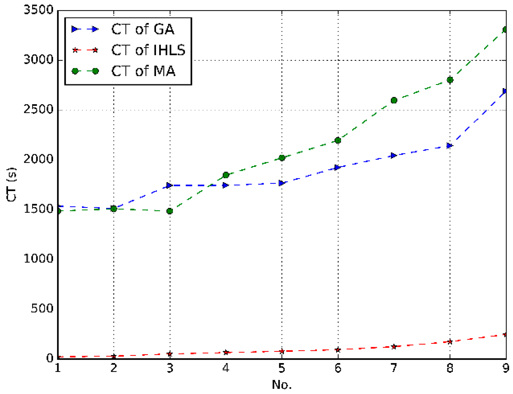
Considering the CPU times of each algorithm in Figure 5, IHLS is the most efficient one among the three algorithms. As shown in Figure 5, the swarm based algorithms, GA and memetic algorithm, are more time-consuming. With the increasing of instance size, the CPU time of memetic algorithm is getting larger, and memetic algorithm become the most time-consuming one.
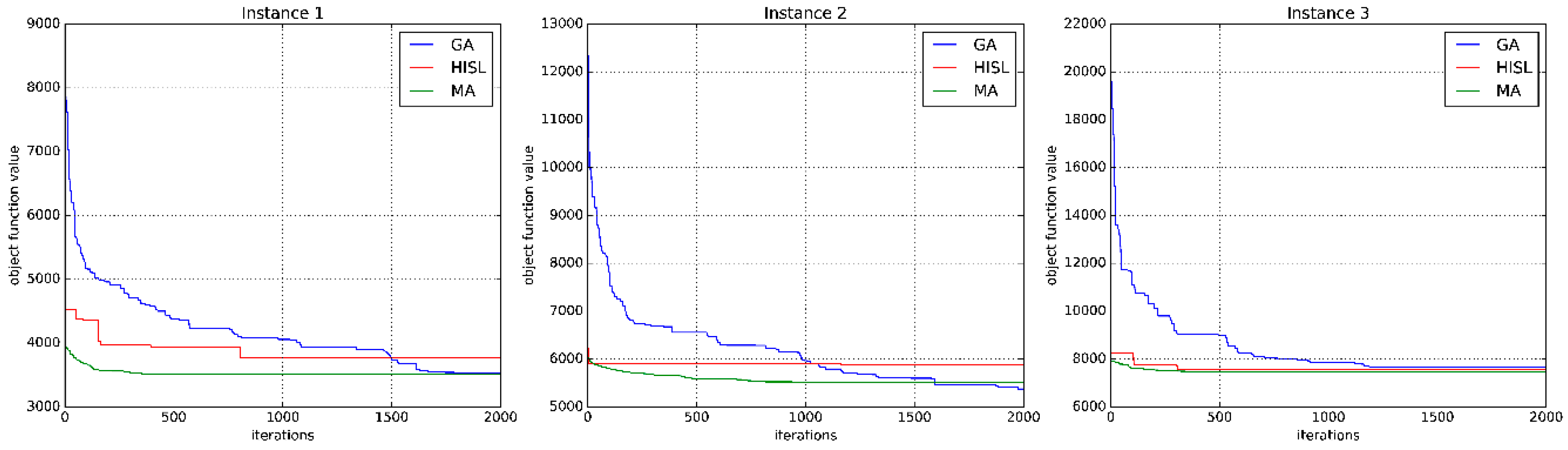
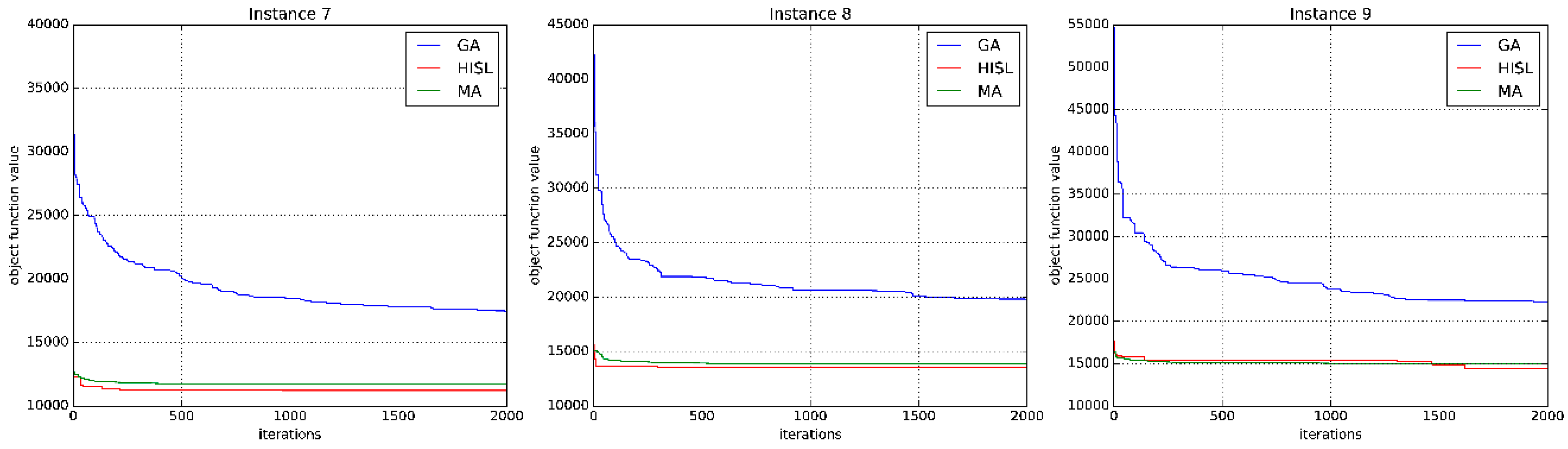
In respect of optimality, IHLS algorithm has an advantage in large-scale instances, while the solution of IHLS is slightly inadequate in small one. In respect of CPU times, IHLS algorithm has a great advantage in both small-scale and large-scale instances. To show the convergence of different heuristics, the stopping criteria is set as 2000 iterations. The convergence plot comparisons of the three algorithms are shown in Figure 6 and Figure 7. Figure 6 shows the convergence plot in solving instance 1, 2 and 3 which are small-size data, while Figure 7 shows the convergence plot in solving instance 7, 8 and 9 which are large-size data. More analysis details will be explained in the following.
To measure IHLS performance, a relative quality measure , where is the best among the solutions obtained by the three algorithms and is IHLS. The closer to 0 the measure value is, the better the according algorithm will be.
As shown in Figure 6, from instance 1 to instance 3, the number of points < 150, there is a flaw in IHLS’ solutions. GA obtained minimum object function value which is the best feasible solution in instance 2, memetic algorithm obtained the best feasible solution in instance 1 and instance 3. In Figure 6 (instance 1), the best solution is 3511 mm, the feasible solution of IHLS is 3766 mm, . Similarly, the measure value is 8.68% in Figure 6 (instance 2). While the measure value in Figure 6 (instance 3), which becomes smaller. Although IHLS lacks good performance in Figure 6, the difference between the IHLS’ object function and the best solution is less than 700. As shown in Figure 7, from instance 7 to instance 9, the number of points , IHLS’s solution is the best among three heuristics. Obviously, the measure value is in Figure 7. In Figure 7, memetic algorithm also has a good performance, but the quality of solution is slightly worse than that of IHLS. The difference between memetic algorithm’s and IHLS’ solution values are 507, 240 and 157 in instance 7, 8 and 9 respectively, while the difference of GA are more than 3000. Figure 6 and Figure 7 show that IHLS lacks good performance in solving small-scale problem, while with the increasing of points number, it demonstrates that IHLS has a better performance in solving large-scale problem.
From instance 1 to 9, both IHLS and memetic algorithm achieve a better convergence value in the first iteration, while the GA’s first convergence value is worse. The solutions of IHLS and memetic algorithm converges relatively rapidly. In addition, IHLS is more suitable for real-time application in operation workshop because of its higher computational efficiency. Considering the time-consuming and optimality, IHLS is superior to memetic algorithms.
5. Conclusions
In this paper, we deal with the pick-and-place optimization problem efficiently by a new algorithm (IHLS) combining local search with integer programming. In the section of local search, the greedy with distance weight strategy and the convex-hull strategy are developed to determine the pick-and-place sequence; in the section of integer programming, an integer programming model is built to solve the feeder assignment. The experimental result shows that the IHLS we proposed has a higher computational efficiency. The IHLS is less time-consuming and more suitable in solving large scale problems. In our future work, in order to improve the accuracy of IHLS in small size data, some other solving techniques could be integrated and the mathematical model should be improved.
Author Contributions
Conceptualization, J.G.; Methodology, J.G. and X.Z.; Software, J.G.; Validation, X.Z.; Writing—Original Draft Preparation, J.G. and A.L.; Writing—Review & Editing, Q.M.; Supervision, X.Z.; Project Administration, R.Z.
Funding
This research was funded by the key program of National Natural Science Foundation of China grant number 71532002.
Acknowledgments
In this section you can acknowledge any support given which is not covered by the author contribution or funding sections. This may include administrative and technical support, or donations in kind (e.g., materials used for experiments).
Conflicts of Interest
The authors declare no conflict of interest.
References
- Li, D.; Yoon, S.W. PCB assembly optimization in a single gantry high-speed rotary-head collect-and-place machine. Int. J. Adv. Manuf. Technol. 2017, 88, 2819–2834. [Google Scholar] [CrossRef]
- Ho, W.; Ji, P.; Wu, Y. A heuristic approach for component scheduling on a high speed PCB assembly machine. Prod. Plan. Control 2007, 18, 655–665. [Google Scholar] [CrossRef]
- Or, I. Precedence constrained TSP arising in printed circuit board assembly. Int. J. Prod. Res. 2004, 42, 67–78. [Google Scholar] [CrossRef]
- Grunow, M.; Schleusener, M.; Yilmaz, I.O. Operations planning for collect-and-place machines in PCB assembly. Comput. Ind. Eng. 2004, 47, 409–429. [Google Scholar] [CrossRef]
- Sun, D.S.; Lee, T.E.; Kim, K.H. Component allocation and feeder arrangement for a dual-gantry multi-head surface mounting placement tool. Int. J. Prod. Econ. 2005, 95, 245–264. [Google Scholar] [CrossRef]
- Wang, C. A dynamic point specification approach to sequencing robot moves for PCB assembly. Int. J. Comput. Integr. Manuf. 1995, 8, 448–456. [Google Scholar] [CrossRef]
- Ancu, M. The optimization of printed circuit board manufacturing by improving the drilling process productivity. Comput. Ind. Eng. 2008, 55, 279–294. [Google Scholar] [CrossRef]
- Shah, H.; Tairan, N.; Garg, H.; Ghazali, R. A Quick Gbest Guided Artificial Bee Colony Algorithm for Stock Market Prices Prediction. Symmetry 2018, 10, 292. [Google Scholar] [CrossRef]
- Połap, D.; Wo’zniak, M. Polar Bear Optimization Algorithm: Meta-Heuristic with Fast Population Movement and Dynamic Birth and Death Mechanism. Symmetry 2017, 9, 203. [Google Scholar] [CrossRef]
- Duan, K.; Fong, S.; Siu, S.W.I.; Song, W.; Guan, S.S.-U. Adaptive Incremental Genetic Algorithm for Task Scheduling in Cloud Environments. Symmetry 2018, 10, 168. [Google Scholar] [CrossRef]
- Hassanat, A.B.; Prasath, V.B.S.; Abbadi, M.A.; Abu-Qdari, S.A.; Faris, H. An Improved Genetic Algorithm with a New Initialization Mechanism Based on Regression Techniques. Information 2018, 9, 167. [Google Scholar] [CrossRef]
- Zhao, H.; Gao, W.; Deng, W.; Sun, M. Study on an Adaptive Co-Evolutionary ACO Algorithm for Complex Optimization Problems. Symmetry 2018, 10, 104. [Google Scholar] [CrossRef]
- Kulak, O.; Yilmaz, I.O.; Günther, H.O. PCB assembly scheduling for collect-and-place machines using genetic algorithms. Int. J. Prod. Res. 2007, 45, 3949–3969. [Google Scholar] [CrossRef]
- Chyu, C.C.; Chang, W.S. A genetic-based algorithm for the operational sequence of a high speed chip placement machine. Int. J. Adv. Manuf. Technol. 2008, 36, 918–926. [Google Scholar] [CrossRef]
- Alkaya, A.F.; Duman, E. Combining and solving sequence dependent traveling salesman and quadratic assignment problems in PCB assembly. Discret. Appl. Math. 2015, 192, 2–16. [Google Scholar] [CrossRef]
- Chen, Y.M.; Lin, C.T. A particle swarm optimization approach to optimize component placement in printed circuit board assembly. Int. J. Adv. Manuf. Technol. 2007, 35, 610–620. [Google Scholar] [CrossRef]
- Zhu, G.Y.; Zhang, W.B. An improved Shuffled Frog-leaping Algorithm to optimize component pick-and-place sequencing optimization problem. Expert Syst. Appl. 2014, 41, 6818–6829. [Google Scholar] [CrossRef]
- Lin, H.Y.; Lin, C.J.; Huang, M.L. Optimization of printed circuit board component placement using an efficient hybrid genetic algorithm. Appl. Intell. 2016, 45, 1–16. [Google Scholar] [CrossRef]
- Han, J.; Seo, Y. Mechanism to minimise the assembly time with feeder assignment for a multi-headed gantry and high-speed SMT machine. Int. J. Prod. Res. 2016, 55, 2930–2949. [Google Scholar] [CrossRef]
- Luo, J.; Liu, J.; Hu, Y. An MILP model and a hybrid evolutionary algorithm for integrated operation optimisation of multi-head surface mounting machines in PCB assembly. Int. J. Prod. Res. 2016, 55, 145–160. [Google Scholar] [CrossRef]
- Kumar, R.; Li, H. Integer programming approach to printed circuit board assembly time optimization. IEEE Trans. Compon. Packag. Manuf. Technol. Part B 1995, 18, 720–727. [Google Scholar] [CrossRef] [Green Version]
- Altinkemer, K.; Kazaz, B.; Köksalan, M. Optimization of printed circuit board manufacturing: Integrated modeling and algorithms. Eur. J. Oper. Res. 2007, 124, 409–421. [Google Scholar] [CrossRef]
- Ho, W.; Ji, P. An integrated scheduling problem of PCB components on sequential pick-and-place machines: Mathematical models and heuristic solutions. Expert Syst. Appl. 2009, 36, 7002–7010. [Google Scholar] [CrossRef]
- Luo, J.; Liu, J. An MILP model and clustering heuristics for LED assembly optimisation on high-speed hybrid pick-and-place machines. Int. J. Prod. Res. 2014, 52, 1016–1031. [Google Scholar] [CrossRef]
- Iantovics, L.B.; Dehmer, M.; Emmert-Streib, F. MetrIntSimil—An Accurate and Robust Metric for Comparison of Similarity in Intelligence of Any Number of Cooperative Multiagent Systems. Symmetry 2018, 10, 48. [Google Scholar] [CrossRef]
- Essani, F.H.; Haider, S. An Algorithm for Mapping the Asymmetric Multiple Traveling Salesman Problem onto Colored Petri Nets. Algorithms 2018, 11, 143. [Google Scholar] [CrossRef]
- Deineko, G.; Woeginger, J. The convex-hull-and-k-line travelling salesman problem. Inf. Process. Lett. 1996, 59, 295–301. [Google Scholar] [CrossRef]
- Cotta, C.; Fernàndez, J. Memetic Algorithms in Planning, Scheduling, and Timetabling. In Evolutionary Scheduling; Springer: Berlin/Heidelberg, Germany, 2007; pp. 1–30. [Google Scholar]
Figure 1.
The main structure of pick-and-place machine.

Figure 2.
The distance weights confirming process.

Figure 3.
The example of adjustment strategy.

Figure 4.
Flowchart of the IHLS algorithm.

Figure 5.
The CPU time of each test algorithm

Figure 6.
The convergent curves in small-size data.

Figure 7.
The convergent curves in large-size data.

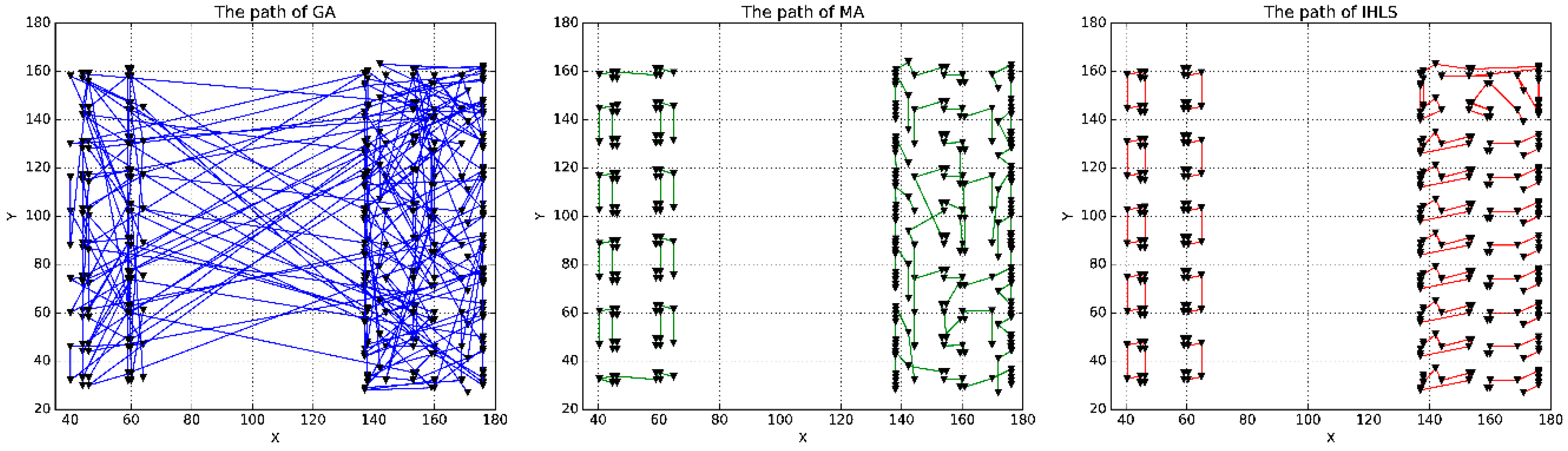
Figure 8.
The path comparison of Instance 9.


Table 1.
The example of greedy strategy with distance weight.
| No. | ||
|---|---|---|
| 1 | 16 | 2 |
| 18 | 2 | |
| 19 | 12 | |
| 17 | 14 | |
| 5 | 11 | 8 |
| 6 | 15 | 4 |
Table 2.
The corresponding .
| 0 | 0 | 0 | 1 | |
| 1 | 0 | 0 | 0 | |
| 0 | 0 | 0 | 0 | |
| 1 | 1 | 0 | 0 |
Table 3.
Comparison of the IHLS results with the optimal solutions.
| (PN, TN) | No. | Object Function Value (mm) | CUP Times | |||
|---|---|---|---|---|---|---|
| (6, 5) | 1 | 280.12 | 263.37 | 6.45 | 0.35 | 0.27 |
| (8, 6) | 2 | 409.41 | 383.71 | 6.78 | 0.98 | 0.83 |
| (10, 6) | 3 | 598.34 | 566.02 | 5.65 | 2.21 | 2.09 |
| (82, 3) | 4 | 3766 | Unsolved | - | 22.3 | - |
Table 4.
The size of instances.
| No. | N | t | H | n | S | (sx, sy) | ||
|---|---|---|---|---|---|---|---|---|
| 1 | 82 | 3 | 10 | 9 | 60 | (−120, −72) | 12 | (10, 10, …, 3) |
| 2 | 100 | 4 | 10 | 10 | 60 | (−120, −72) | 12 | (10, 10, …, 10) |
| 3 | 145 | 5 | 10 | 15 | 60 | (−120, −72) | 12 | (10, 10, …, 5) |
| 4 | 163 | 4 | 10 | 17 | 60 | (−120, −72) | 12 | (10, 10, …, 3) |
| 5 | 184 | 5 | 10 | 19 | 60 | (−120, −72) | 12 | (10, 10, …, 4) |
| 6 | 200 | 5 | 10 | 20 | 60 | (−120, −72) | 12 | (10, 10, …, 10) |
| 7 | 240 | 6 | 10 | 24 | 60 | (−120, −72) | 12 | (10, 10, …, 10) |
| 8 | 264 | 7 | 10 | 27 | 60 | (−120, −72) | 12 | (10, 10, …, 4) |
| 9 | 300 | 9 | 10 | 30 | 60 | (−120, −72) | 12 | (10, 10, …, 10) |
Table 5.
Experimental results of different size data.
| No. | GA | IHLS | Memetic Algorithm | |||||
|---|---|---|---|---|---|---|---|---|
| 1 | 3511 | 22.3 | 3542 | 1534.0 | 3766 | 22.3 | 3511 | 1485.7 |
| 2 | 5509 | 29.5 | 5377 | 1512.4 | 5844 | 29.5 | 5509 | 1508.2 |
| 3 | 7473 | 52.4 | 7655 | 1743.5 | 7740 | 52.4 | 7473 | 1485.0 |
| 4 | 8166 | 65.0 | 8352 | 1744.0 | 8479 | 65.0 | 8166 | 1846.8 |
| 5 | 8813 | 78.4 | 10,439 | 1766.8 | 8813 | 78.4 | 9430 | 2020.5 |
| 6 | 9882 | 93.4 | 11,541 | 1923.4 | 9882 | 93.4 | 10,249 | 2195.0 |
| 7 | 11,218 | 124.2 | 14,745 | 2043.8 | 11,218 | 124.2 | 11,725 | 2596.0 |
| 8 | 13,591 | 174.2 | 17,610 | 2142.0 | 13,591 | 174.2 | 13,837 | 2802.0 |
| 9 | 14,854 | 247.0 | 20,745 | 2689.4 | 14,854 | 247.0 | 15,007 | 3310.7 |
Table 6.
Results of IHLS in instance 9.
| Corresponding Feeder Type | Corresponding Feeder Coordinates | |||
|---|---|---|---|---|
| 1 | 100004652 | (192, −72) | ||
| 2 | 100004697 | (144, −72) | ||
| 3 | 100004795 | (156, −72) | ||
| 4 | 100004883 | (180, −72) | ||
| 5 | 100005022 | (16, −72) | ||
| 6 | 100006424 | (−96, −72) | ||
| 7 | 100008025 | (132, −72) | ||
| 8 | 100030843 | (168, −72) | ||
| 9 | 100031371 | (48, −72) | ||
| 10 | ||||
| 11 | ||||
| 12 | ||||
| 13 | ||||
| 14 | ||||
| 15 | ||||
| 16 | ||||
| 17 | ||||
| 18 | ||||
| 19 | ||||
| 20 | ||||
| 21 | ||||
| 22 | ||||
| 23 | ||||
| 24 | ||||
| 25 | ||||
| 26 | ||||
| 27 | ||||
| 28 | ||||
| 29 | ||||
| 30 |
© 2018 by the authors. Licensee MDPI, Basel, Switzerland. This article is an open access article distributed under the terms and conditions of the Creative Commons Attribution (CC BY) license (http://creativecommons.org/licenses/by/4.0/).
Share and Cite
MDPI and ACS Style
Gao, J.; Zhu, X.; Liu, A.; Meng, Q.; Zhang, R. An Iterated Hybrid Local Search Algorithm for Pick-and-Place Sequence Optimization. Symmetry 2018, 10, 633. https://doi.org/10.3390/sym10110633
AMA Style
Gao J, Zhu X, Liu A, Meng Q, Zhang R. An Iterated Hybrid Local Search Algorithm for Pick-and-Place Sequence Optimization. Symmetry. 2018; 10(11):633. https://doi.org/10.3390/sym10110633
Chicago/Turabian StyleGao, Jinsheng, Xiaomin Zhu, Anbang Liu, Qingyang Meng, and Runtong Zhang. 2018. "An Iterated Hybrid Local Search Algorithm for Pick-and-Place Sequence Optimization" Symmetry 10, no. 11: 633. https://doi.org/10.3390/sym10110633
Note that from the first issue of 2016, this journal uses article numbers instead of page numbers. See further details here.