Weak Fault Detection for Gearboxes Using Majorization–Minimization and Asymmetric Convex Penalty Regularization

Abstract

It is a primary challenge in the fault diagnosis community of the gearbox to extract the weak fault features under heavy background noise and nonstationary conditions. For this purpose, a novel weak fault detection approach based on majorization–minimization (MM) and asymmetric convex penalty regularization (ACPR) is proposed in this paper. The proposed objective cost function (OCF) consisting of a signal-fidelity term, and two parameterized penalty terms (i.e., one is an asymmetric nonconvex penalty regularization term, and another is a symmetric nonconvex penalty regularization term).To begin with, the asymmetric and symmetric penalty functions are established on the basis of an L1-norm model, then, according to the splitting idea, the majorizer of the symmetric function and the majorizer of the asymmetric function are respectively calculated via the MM algorithm. Finally, the MM is re-introduced to solve the proposed OCF. As examples, the effectiveness and reliability of the proposed method is verified through simulated data and gearbox experimental real data. Meanwhile, a comparison with the state of-the-art methods is illustrated, including nonconvex penalty regularization (NCPR) and L1-norm fused lasso optimization (LFLO) techniques, the results indicate that the gear chipping characteristic frequency 13.22 Hz and its harmonic (2f, 3f, 4f and 5f) can be identified clearly, which highlights the superiority of the proposed approach.

1. Introduction

Gearboxes are widely used in transmission systems with rotating machinery, due to its advantages, such as a high transmission ratio and large load capacity, which plays an important role in modern industrial applications. Unexpected bearing failure caused by a harsh working environment and intricate running conditions may result in catastrophic incidents, significant economic losses, and even human casualties. Thus, timely and precise condition-based monitoring (CBM) and health assessments of rotating machines are of great significance in practice, performed online or offline, to avoid a mechanical breakdown, especially in the early stages of failure [1,2,3].

The vibration signal generated by localized faults is a typical non-linear and non-stationary signal; thus, fault feature extraction based on vibration signal has become the mainstream technique in the fault diagnosis field. However, the observed vibration signals are usually corrupted by severe background noise and interference components. For the purpose of detecting fault from rotating machines, over the past decades, numerous diagnostic techniques have been developed. For example, some methods are used via signal transforms, such as wavelet/wavelet packet transform [4,5,6], short-time Fourier transform [7,8], or tunable Q-factor wavelet transform (TQWT) [9,10]. Some methods are used via signal adaptive decomposition, such as empirical mode decomposition (EMD) [11,12], local mean decomposition (LMD) [13,14], and variational mode decomposition (VMD) [15,16]; in addition, some methods are used by intelligent supervised learning techniques, such as artificial neural network (ANN) [17,18], deep learning (DL) [19,20], just to mention a few. These methods have achieved successful applications in fault diagnosis of rotating machinery to some extent.

Compared to the above conventional fault feature extraction approaches, most recently, sparse coding techniques (SCT) or sparse representation (SR) as a new fault detection method was introduced for fault feature extraction and condition monitoring [21,22]. By applying the SR approach, the observed vibration signals can be represented as a linear combination of a few sparse bases (e.g., wavelet base) or sparse atoms generated by an over-complete dictionary (OCD), so the instantaneous fault impulses can be substituted by a few sparse coefficients. Zhou et al. [23] proposed shift-invariant dictionary learning (SIDL) and a hidden Markov model (HMM) to address bearing fault diagnosis and identify fault types. Further, Yang et al. [24] and Feng et al. [25] proposed a shift-invariant K-singular value decomposition (SI-K-SVD) method combined with a sparse representation algorithm to extract the fault impulse of wind turbine generator bearing and planetary gearbox fault, respectively. Qin [26] developed the model-based impulsive wavelet basis and Fourier basis for the weak repetitive transient feature extraction of a rolling bearing. The adaptive impulse dictionary, double-dictionary matching pursuit (DDMP), and step-impulse dictionary were introduced for detecting the physical defect size of the inner and outer race of a rolling bearing in [27,28,29]. Ding et al. [30] employed the time-frequency (TF) dictionary and orthogonal matching pursuit (OMP) to extract the fault feature information of single row cylindrical roller bearings based on acoustic signals. Li et al. [31] introduced a novel dictionary learning method called the impulse-step impact dictionary, based on a nonconvex optimization approach; the results demonstrate the method’s superiority in weak fault feature extraction via accelerated lifetime testing experiment, compared with OMP, L1-norm convex penalty regularization, and the spectral Kurtogram (SK) method.

Although the above SR and its extension, combined with the redundant dictionary, have achieved satisfactory applications in fault diagnosis, those algorithms have some common drawbacks:

(1)

Unique dictionaries’ atoms and optimal wavelet basis cannot simultaneously match the natural structure of every real vibration signal well;

(2)

A large number of observed signals should be collected to form a training dictionary before diagnosis, which is always infeasible in practical applications;

(3)

Computational complexity and time-consuming problems occur simultaneously in dictionary training, such as with the K-SVD training and SI-K-SVD dictionaries training [31].

In an attempt to overcome the above shortcomings of an over-complete dictionary (OCD) and estimate the fault characteristics more accurately, the family of low-rank matrix approximation (LRMA) methods were introduced in recent years, Thus the reconstruction problem of dictionary atoms is translated into an optimization or inverse regularization problem. In [32], Ding et al. propose an algorithm that combines alternating the direction method of multipliers (ADMM) and the majorization–minimization (MM) method to compute a low-rank matrix optimization model. In [33] and [34], He et al. develop nonconvex penalty regularization and a sparsity-based group-sparse signal denoising (OGS) approach to extract the single and compound features of outer and inner race defects. In [35], Zhang et al. proposed a novel convex penalty regularization method called Kurtosis-based weighted sparse decomposition (Kur-WSD) on the basis of the L1-norm method to detect the inner fault of an alternating current motor. In [36], Du et al. propose a rigorously weighted low-rank sparse detection framework to explore the physical/internal mechanisms of bearing faults and implement fault diagnosis of a wind turbine.

Unfortunately, the above low-rank matrix approximation approach still suffers from the following challenges, which have restricted its application development:

(1)

Generally, the penalty functions that are established in a low-rank matrix approximation (LRMA) model are symmetric functions, e.g., the absolute value function (AVF); the common drawback is that this penalty function is non-differentiable at the zero point, which can lead to some numerical issues, such as a local optimum and early termination of algorithm.

(2)

In a conventional low-rank matrix approximation (LRMA) method, the convex regularizer, such as the L1-norm, usually underestimates the sparse signal when the absolute value function (AVF) is used as a sparsity regularizer; the nonconvex regularizer suffers from several issues, such as a strict convexity problem of objective cost function (OCF), a non-convergence problem, etc. Additionally, both the convex and nonconvex regularizers shrink all the coefficients equally and remove too much energy from the useful signal, resulting in the estimation of the fault signal becoming more challenging.

(3)

When the useful fault characteristics signals are very weak but additive noise extremely strong, the conventional LRMA method cannot estimate low-dimensional feature distribution accurately.

Aiming at the issue of estimating the weak fault signal from its noisy observations, and enlightened by the LRMA method, a novel detection approach based on asymmetric convex penalty regularization (ACPR) and majorization–minimization (MM) is proposed in this paper, using the weak chipping fault of a gearbox as a research object. The proposed ACPR method neither relies on the reconstruction of dictionary atoms, nor requires a large number of sample data to form a certain training dictionary; meanwhile, the numerical issues, such as being non-differentiable at zero point, are addressed by introducing the asymmetric convex penalty function. In the modeling solution process, MM is implemented to solve a relatively complicated sparsity-based optimization problem. Finally, the proposed method is validated via the weak fault feature of the simulation and the gearbox dataset collected in the lab experiment; the results of fault frequency and its harmonics indicate that the ACPR method is superior to the other LRMA methods, such as nonconvex penalty regularization (NCPR) and L1-norm fused lasso optimization (LFLO) techniques.

The layout of this work is organized as follows. Section 2 introduces the MM algorithm. Section 3 introduces the algorithm and theoretical derivation of asymmetric convex penalty regularization (ACPR). The simulation evaluation of the proposed method is presented in Section 4. In Section 5, the practical diagnosis results and the discussion of the gearbox using the proposed approach with other LRMA methods are presented. Conclusions are drawn in Section 6.

2. Majorization–Minimization Algorithm

Before the derivation of the proposed algorithm, a review to the majorization–minimization (MM) algorithm is given. Usually, the MM algorithm is used to reduce the computational complexity—in other words, for a minimization problem that is too complex to solve directly, the MM method can simplify it into a series of simpler problems by constructing the majorization functions [37,38,39].

Suppose F(u) is the minimization problem, which is too complex to solve directly. The MM algorithm constructs a simple function G(u, u^k), G(u, u^k), which is called the majorization function of F(u) at the k-th iteration point u^k. More specifically, consider the minimization problem

$$u^{\mathrm{opt}}=\arg \underset{u}{\min }F(u)$$

(1)

By using the MM method, the above problem can be described by the following iteration:

$$u^{(k+1)}=\arg \underset{u}{\min }G(u,u^{(k)})$$

(2)

where k is the iteration number and G(u, u^k) is a continuously differentiable function, satisfying

$$\begin{array}{l}G(u,v)\ge F(u),\mathrm{for}\mathrm{all}u,v,\\ G(u,u)=F(u)\end{array}$$

(3)

Note that the majorizer G(u, v) reaches F(u) for u = v. According to Equations (2) and (3), we have

$$F(u^{k+1})\le G(u^{k+1},u^k)\le G(u^k,u^k)=F(u^k)$$

(4)

This iteration briefly describes the MM approach for minimizing a minimization problem function. The MM algorithm consists of two processes: the construction of the majorization function and the optimization of the majorization function. The main steps of the MM algorithm can be summarized as follows:

(1)

Initialize u⁰ and k = 0;

(2)

Construct a majorization function G(u, u^k);

(3)

Operate the iteration $u^{(k+1)}=\arg \underset{u}{\min }G(u,u^{(k)})$;

(4)

If the stopping criterion is satisfied, then output $u^{\mathrm{opt}}$; otherwise, k = k + 1, and go to step (2);

(5)

Output $u^{\mathrm{opt}}$.

3. Asymmetric Convex Penalty Regularization Algorithm

3.1. Sparse Representation and Filter Banks

Generally, the noisy noisy vibration signal y of rotating machinery, such as a rolling bearing, contains three parts: the fault transient impulses x, the systematic natural vibration signal f, and the additive noise w, i.e.,

$$y=x+f+w$$

(5)

The core work of the fault diagnosis is to extract the fault transient impulses x from the noisy observation y. Assuming that fault transient component impulses and the systematic natural vibration signal are estimated, we have

$$\stackrel{\wedge }{x}\approx x,\stackrel{\wedge }{f}\approx f$$

(6)

Assuming that the estimation of fault transient impulses x is obtained as $\stackrel{\wedge }{x}$, we can estimate signal f as follows:

$$\stackrel{\wedge }{f}=\mathit{L}\mathit{P}\mathit{F}(y-\stackrel{\wedge }{x})$$

(7)

where LPF is a specified low-pass filter. Substituting Equation (7) into $\stackrel{\wedge }{f}\approx f$, we have

$$\mathit{L}\mathit{P}\mathit{F}(y-\stackrel{\wedge }{x})\approx f$$

(8)

Substituting $y=x+f+w$ into $\mathit{L}\mathit{P}\mathit{F}(y-\stackrel{\wedge }{x})\approx f$, we have

$$\begin{array}{l}y\approx x+\mathit{L}\mathit{P}\mathit{F}(y-\stackrel{\wedge }{x})+w\\ \Rightarrow \mathit{L}\mathit{P}\mathit{F}(y-\stackrel{\wedge }{x})\approx y-x-w\end{array}$$

(9)

Substituting $\stackrel{\wedge }{x}\approx x$ into $\mathit{L}\mathit{P}\mathit{F}(y-\stackrel{\wedge }{x})\approx y-x-w$, we have

$$\mathit{L}\mathit{P}\mathit{F}(y-\stackrel{\wedge }{x})\approx y-\stackrel{\wedge }{x}-w\iff (\mathit{I}-\mathit{L}\mathit{P}\mathit{F})(y-\stackrel{\wedge }{x})\approx w$$

(10)

Defining $\mathit{H}\mathit{P}\mathit{F}=\mathit{I}-\mathit{L}\mathit{P}\mathit{F}=H$, thus, we get

$$\mathit{H}\mathit{P}\mathit{F}(y-\stackrel{\wedge }{x})\approx w\Rightarrow \mathit{H}(y-\stackrel{\wedge }{x})\approx w$$

(11)

On the other hand, it should be noted that Equation (5) belongs to a highly underdetermined equation, i.e., an ill-posed or N-P hard problem [40,41,42], for which there are infinite sets of solutions because the number of unknowns is greater than the number of equations. Usually, convex optimization approaches are commonly used to estimate a transient component from the noisy signal; based on the aforementioned work, the estimation of x can be formulated as the constrained optimization problem, i.e.,

$$\stackrel{\wedge }{x}=\arg \underset{x}{\min }\{\frac{1}{2}{\Vert \mathit{H}(y-x)\Vert }_2^2+\lambda {\Vert \mathit{D}x\Vert }_1\}$$

(12)

where H is a specified high-pass filter (i.e., the HPF in Equation (11)), λ is a regularization parameter, and D is a matrix defined as $\mathit{D}=\left[\begin{array}{cccc}-1,1& & & \\ & \cdots & & \\ & & \cdots & \\ & & & -1,1\end{array}\right]$, which controls the sparsity of the approximating value of x. If x is a sparse signal, i.e., most of the amplitude values in x tend to zero, then the problem in Equation (12) can also be solved by the L1-norm fused lasso optimization (LFLO) algorithm, i.e.,

$$\stackrel{\wedge }{x}=\arg \underset{x}{\min }\{\frac{1}{2}{\Vert \mathit{H}(y-x)\Vert }_2^2+{\lambda }_0{\Vert x\Vert }_1+{\lambda }_1{\Vert \mathit{D}x\Vert }_1\}$$

(13)

where λ₀ and λ₁ are regularization parameters. The solution of the LFLO algorithm can be given by a soft-threshold function [43]. In that case, we have

$$x=\mathrm{soft}(\mathrm{tvd}(y,{\lambda }_2),{\lambda }_1)$$

(14)

where function $\mathrm{tvd}(\cdot ,\cdot )$ is the total variation de-noising (TVD) algorithm [44,45,46], and the soft-threshold function is defined as follows

$$\mathrm{soft}(x,\lambda )=\{\begin{array}{ll}x-\lambda \frac{x}{\left|x\right|},\hspace{0.17em}& \left|x\right|>\lambda \\ 0,& \left|x\right|\le \lambda \end{array}$$

(15)

In addition, the high-pass filter H described above could be formulated as follows [45,46,47]:

$$\mathit{H}={\mathit{A}}^{-1}\mathit{B}$$

(16)

where A and B are Toeplitz matrices.

3.2. Asymmetric Convex Penalty Regularization Model

Compared with optimization algorithms Equations (12) and (13), in order to estimate the fault transient impulses x precisely, this work introduces a novel penalty regularization method, i.e., an asymmetric and symmetric nonconvex penalty regularization model:

$$\begin{array}{l}\stackrel{\wedge }{x}=\arg \underset{x}{\min }\{F(x)=\frac{1}{2}{\Vert \mathit{H}(y-x)\Vert }_2^2+{\lambda }_0{\displaystyle \sum _{n=0}^{N-1}{\theta }_{\epsilon }(x_n;r)}\\ +{\displaystyle \sum _{i=1}^M{\lambda }_i}{\displaystyle \sum _{n=0}^{N-1}\varphi ({[{\mathit{D}}_{i}x]}_n)}>\}\end{array}$$

(17)

where F(x) is the proposed objective cost function (OCF), the penalty function ${\theta }_{\epsilon }(x_n;r)$ is a asymmetric and differentiable function, and $\varphi ({[{\mathit{D}}_{i}x]}_n)$ is a symmetric and differentiable function, if the term M = 2, the matrix D₁ is defined as ${\mathit{D}}_1=\left[\begin{array}{cccc}-1,1& & & \\ & \cdots & & \\ & & \cdots & \\ & & & -1,1\end{array}\right]$, and the matrix D₂ is defined as ${\mathit{D}}_2=\left[\begin{array}{cccccc}-1,& 2,& -1& & & \\ & -1,& 2,& -1& & \\ & & & \cdots & & \\ & & & -1,& 2,& -1\end{array}\right]$. The innovations of the novel compound regularizer model are as follows:

(I)

The M-term compound regularizers estimate the fault transient impulses;

(II)

The compound regularizers model consists of symmetric and asymmetric penalty functions, wherein the symmetric penalty function is a differentiable function, compared with the nondifferentiable function $\Vert x_i\Vert$ at i = 0.

(III)

The MM algorithm is introduced for the solution of the proposed compound regularization method.

Based on this, therefore, the core tasks of the proposed algorithm are (1) how to construct a symmetric and differentiable penalty function; (2) how to construct an asymmetric and differentiable penalty function; and (3) how to solve the proposed method based on the MM algorithm and the estimation x, and make diagnosis results more accurately than the traditional LFLO and nonconvex penalty regularization approaches.

For the first task, traditional LFLO regularization approach uses the absolute value function (AVF) ${\varphi }_A(x)=\Vert x\Vert$ as the penalty function; however, the common drawback of ${\varphi }_A(x)=\Vert x\Vert$ is that this function is non-differentiable at zero point, which can cause some numerical problems. To address this issue, some non-linear approximation functions of ${\varphi }_A(x)=\Vert x\Vert$ are proposed, i.e.,

$${\varphi }_B(x)=\sqrt{{\left|x\right|}^2+\epsilon }$$

(18)

Or

$${\varphi }_c(x)=\left|x\right|-\epsilon \log (\left|x\right|+\epsilon )$$

(19)

Note that when $\epsilon =0$, then the ${\varphi }_B(x)$ and ${\varphi }_c(x)$ degrade into the AVF ${\varphi }_A(x)$, and while the $\epsilon >0$, the ${\varphi }_B(x)$ and ${\varphi }_c(x)$ are differentiable at the zero point. The functions ${\varphi }_A(x)$, ${\varphi }_B(x)$, ${\varphi }_c(x)$, and their first-order derivatives are listed in

Table 1. Symmetric penalty functions and their derivatives.

Functions	$\mathit{\varphi }\mathbf{(}\mathit{x}\mathbf{)}$	${\mathit{\varphi }}^{\mathbf{\prime }}\mathbf{(}\mathit{x}\mathbf{)}$
${\varphi }_A(x)$	$\Vert x\Vert$	Signal(x)
${\varphi }_B(x)$	$\sqrt{{\left|x\right|}^2+\epsilon }$	$x/\sqrt{{\left|x\right|}^2+\epsilon }$
${\varphi }_c(x)$	$\left|x\right|-\epsilon \log (\left|x\right|+\epsilon )$	$x/(\left|x\right|+\epsilon )$

.

In order for the non-linear approximation functions to maintain the reliable sparsity-inducting behavior of the original LFLO algorithm, the parameter $\epsilon$ should be set to an adequately small positive value. For example, the parameters $\epsilon ={10}^{-5}$ and $\epsilon ={10}^{-6}$ are small enough that numerical issues can be avoided, and their impact on the sparsity promoting can also be ignored.

For the second task, inspired by the AVF ${\varphi }_A(x)=\Vert x\Vert$, and in contrast to the symmetric and differentiable penalty function ${\varphi }_B(x)$ and ${\varphi }_c(x)$, here a segmented function is proposed as follows:

$${\theta }_{\epsilon }(x)=\{\begin{array}{ll}x,& x>\epsilon \\ f(x),& \Vert x\Vert \le \epsilon \\ -rx,& x<\epsilon \end{array}$$

(20)

where $r>0$ is a positive constant. Therefore, the main problem of Equation (20) will transforms into a task about how to construct the intermediate function $f(x),-\epsilon \le x\le \epsilon$. To address this issue, we seek a majorizer as the approximation function of $f(x),-\epsilon \le x\le \epsilon$; here, in order to eliminate the issue that the penalty function is non-differentiable at zero point, a simple quadratic equation (QE) is introduced accordingly,

$$g(x,v)=a{x}^2+bx+c$$

(21)

According to the theory of the majorization–minimization (MM), we have,

$$\begin{array}{l}g(v,v)=\theta (v,r),g^{\prime }(v,v)={\theta }^{\prime }(v,r)\\ g(s,v)=\theta (s,r),g^{\prime }(s,v)={\theta }^{\prime }(s,r)\end{array}$$

(22)

The parameters a, b, c and s are all function of v, and solving for them gives

$$a=\frac{1+r}{4\left|v\right|},b=\frac{1-r}{2},c=\frac{(1+r)\left|v\right|}{4},s=-v$$

(23)

Substituting Equation (23) into $g(x,v)=a{x}^2+bx+c$, we have

$$g(x,v)=\frac{1+r}{4\left|v\right|}{x}^2+\frac{1-r}{2}x+\frac{(1+r)\left|v\right|}{4}$$

(24)

Similarly, the numerical issue of Equation (24) will appear if the parameter v approaches zero. To address this issue, the sufficiently small positive value $\epsilon$ is used instead of $\left|v\right|$; thus, the segmented function Equation (20) can be rewritten as,

$${\theta }_{\epsilon }(x)=\{\begin{array}{ll}x,& x>\epsilon \\ \frac{1+r}{4\epsilon }{x}^2+\frac{1-r}{2}x+\frac{(1+r)\epsilon }{4},\hspace{0.17em}& \Vert x\Vert \le \epsilon \\ -rx,& x<\epsilon \end{array}$$

(25)

Hence, the new function ${\theta }_{\epsilon }(x)$ is a continuously differentiable function.

The third task will be solved and derived in Section 3.3 using the MM algorithm.

3.3. The Solution of the Proposed Model Based on the Majorization–Minimization Algorithm

In this paper, the majorization–minimization (MM) algorithm is implemented to derive an iterative solution procedure for the proposed approach [47]. The function G(x, v) is chosen as the majorizer of F(x). Specifically, the iterative solution procedure can be could be divided into three phases:

(a)

The majorizer of the symmetric and differentiable function $\varphi ({[{\mathit{D}}_{i}x]}_n)$ based on the MM algorithm.

(b)

The majorizer of the asymmetric and differentiable function ${\theta }_{\epsilon }(x_n;r)$ based on the MM algorithm.

(c)

The majorizer of the objective cost function F(x) based on the MM algorithm.

For problem (a), we first seek the majorizer $g(x,v)$ for $\varphi (x)$, i.e.,

$$\begin{array}{l}g(v,v)=\varphi (v),\mathrm{for}\mathrm{all}x,v\\ g(x,v)\ge \varphi (x)\end{array}$$

(26)

Since $\varphi (x)$ is symmetric function, we set $g(x,v)$ to be an even second-order polynomial, i.e.,

$$g(x,v)=m{x}^2+b$$

(27)

Thus, according to Equation (26), as well as $g(v,v)=\varphi (v)$ and $g^{\prime }(v,v)={\varphi }^{\prime }(v)$, we have

$$m{x}^2+b=\varphi (v)\mathrm{and}2mv={\varphi }^{\prime }(v)$$

(28)

The parameters m and b can be computed as

$$m=\frac{{\varphi }^{\prime }(v)}{2v}\mathrm{and}b=\varphi (v)-\frac{v}{2}{\varphi }^{\prime }(v)$$

(29)

Substituting Equation (29) into Equation (27), we have

$$g(x,v)=\frac{{\varphi }^{\prime }(v)}{2v}{x}^2+\varphi (v)-\frac{v}{2}{\varphi }^{\prime }(v)$$

(30)

In summation, we obtain

$$\begin{array}{l}{\displaystyle \sum _{n}g(x_n,v_n)}={\displaystyle \sum _n[\frac{{\varphi }^{\prime }(v_n)}{2v_n}{x}_n{}^2+\varphi (v_n)-\frac{v_n}{2}{\varphi }^{\prime }(v_n)]}\\ =\frac{1}{2}{x}^T\frac{{\varphi }^{\prime }(v_n)}{v_n}x+{\displaystyle \sum _n[\varphi (v_n)-\frac{v_n}{2}{\varphi }^{\prime }(v_n)]}\\ =\frac{1}{2}{x}^T{[\mathbf{\Lambda }(v)]}_{n}x+c(v)\\ \ge {\displaystyle \sum _{n=0}^{N-1}\varphi (x_n)}\end{array}$$

(31)

where ${[\mathbf{\Lambda }(v)]}_n=\frac{{\varphi }^{\prime }(v_n)}{v_n}$ is diagonal matrix and $c_i({\mathit{D}}_{i}v)={\displaystyle \sum _n[\varphi ({[{\mathit{D}}_{i}v]}_n)-\frac{{[{\mathit{D}}_{i}v]}_n}{2}{\varphi }^{\prime }({[{\mathit{D}}_{i}v]}_n)]}$. Therefore, based on Equation (31), we obtain

$$\begin{array}{l}{\displaystyle \sum _{i=0}^M{\lambda }_i}{\displaystyle \sum _{n=0}^{N-1}g({[{\mathit{D}}_{i}x]}_n,{[{\mathit{D}}_{i}v]}_n)}\\ ={\displaystyle \sum _{i=0}^M[\frac{{\lambda }_i}{2}{({\mathit{D}}_{i}x)}^T[\frac{{\varphi }^{\prime }({\mathit{D}}_{i}v)}{{\mathit{D}}_{i}v}]({\mathit{D}}_{i}x)+{\displaystyle \sum _n[\varphi ({[{\mathit{D}}_{i}v]}_n)-\frac{{[{\mathit{D}}_{i}v]}_n}{2}{\varphi }^{\prime }({[{\mathit{D}}_{i}v]}_n)}]]}\\ ={\displaystyle \sum _{i=0}^M[\frac{{\lambda }_i}{2}{({\mathit{D}}_{i}x)}^T[\mathbf{\Lambda }({\mathit{D}}_{i}v)]({\mathit{D}}_{i}x)+c_i({\mathit{D}}_{i}v)]}\\ \ge {\displaystyle \sum _{i=0}^M{\lambda }_i}{\displaystyle \sum _{n=0}^{N-1}\varphi ({[{\mathit{D}}_{i}x]}_n)}\end{array}$$

(32)

where ${[\mathbf{\Lambda }({\mathit{D}}_{i}v)]}_n=\frac{{\varphi }^{\prime }({[{\mathit{D}}_{i}v]}_n)}{{[{\mathit{D}}_{i}v]}_n}$ is a diagonal matrix and $c({\mathit{D}}_{i}v)={\displaystyle \sum _n[\varphi ({[{\mathit{D}}_{i}v]}_n)-\frac{{[{\mathit{D}}_{i}v]}_n}{2}{\varphi }^{\prime }({[{\mathit{D}}_{i}v]}_n)]}$.

For problem (b), we assume that $g_0(x,v)$ is the majorizer of the asymmetric and differentiable function ${\theta }_{\epsilon }(x_n;r)$; since $f(x)=\frac{1+r}{4\epsilon }{x}^2+\frac{1-r}{2}x+\frac{(1+r)\epsilon }{4},\Vert x\Vert \le \epsilon$, we have

$$\{\begin{array}{ll}{g}_0(x,v)=\frac{1+r}{4v}{x}^2+\frac{1-r}{2}x+\frac{(1+r)v}{4}\ge f(x),& v>\epsilon \\ g_0(x,v)=-\frac{1+r}{4v}{x}^2+\frac{1-r}{2}x-\frac{(1+r)v}{4}\ge f(x),& v<-\epsilon \end{array}$$

(33)

when $v<-\epsilon$, then

$$\begin{array}{l}{g}_0(x,v)-f(x)=(\frac{1+r}{4v}-\frac{1+r}{4\epsilon })x^2+(v-\epsilon )\frac{1+r}{4}\\ =\frac{(1+r)(v-\epsilon )(v\epsilon -x^2)}{4v\epsilon }>0\end{array}$$

(34)

when $v<\epsilon$, then

$$\begin{array}{l}{g}_0(x,v)-f(x)=(-\frac{1+r}{4v}-\frac{1+r}{4\epsilon })x^2-(v+\epsilon )\frac{1+r}{4}\\ =-\frac{(1+r)(v+\epsilon )(v\epsilon +x^2)}{4v\epsilon }>0\end{array}$$

(35)

Therefore, the majorizer of the asymmetric and differentiable function ${\theta }_{\epsilon }(x_n;r)$ is obtained:

$$\{\begin{array}{ll}{g}_0(x,v)=\frac{1+r}{4\left|v\right|}{x}^2+\frac{1+r}{2}x+\left|v\right|\frac{1+r}{4},& \left|v\right|>\epsilon \\ g_0(x,v)=\frac{1+r}{4\epsilon }{x}^2+\frac{1+r}{2}x+\epsilon \frac{1+r}{4},\hspace{0.17em}& \left|v\right|\le \epsilon \end{array}$$

(36)

In summation, we obtain

$$\begin{array}{l}{\displaystyle \sum _{n=0}^{N-1}{g}_0(x_n,v_n)}=x^T[\mathbf{\Gamma }(v)]x+b^{T}x+c(v)\\ \ge {\displaystyle \sum _{n=0}^{N-1}{\theta }_{\epsilon }(x_n,r)}\end{array}$$

(37)

where $\mathbf{\Gamma }(v)$ is a diagonal matrix, i.e., ${[\mathbf{\Gamma }(v)]}_n=(1+r)/4\left|v_n\right|,\left|v_n\right|\ge \epsilon$ and ${[\mathbf{\Gamma }(v)]}_n=(1+r)/4\epsilon ,\left|v_n\right|\le \epsilon$, and ${[b]}_n=(1-r)/2$.

For problem (c), based on Equations (32) and (37), the majorizer of F(x) based on the MM algorithm is given by

$$\begin{array}{l}G(x,v)=\frac{1}{2}{\Vert H(y-x)\Vert }_2^2+{\lambda }_0{x}^T[\mathbf{\Gamma }(v)]x+{\lambda }_0{b}^{T}x\\ +{\displaystyle \sum _{i=1}^M\left[\frac{{\lambda }_i}{2}{({\mathit{D}}_{i}x)}^T[\mathbf{\Lambda }({\mathit{D}}_{i}v)]({\mathit{D}}_{i}x)\right]}+c(v)\end{array}$$

(38)

Minimizing G(x, v) with respect to x yields

$$x=H^{T}H+2{\lambda }_0\mathbf{\Gamma }(v)+{\displaystyle \sum _{i=1}^M{\lambda }_i{\mathit{D}}_i^T{[\mathbf{\Lambda }({\mathit{D}}_{i}v){\mathit{D}}_i]}^{-1}(H^{T}Hy-{\lambda }_{0}b)}$$

(39)

Here, substituting H = BA⁻¹ into Equation (39), we have

$$\begin{array}{l}x=\mathit{A}{\{{\mathit{B}}^T\mathit{B}+{\mathit{A}}^T(2{\lambda }_0\mathbf{\Gamma }(v)+{\displaystyle \sum _{i=1}^M{\lambda }_i{\mathit{D}}_i^T[\mathbf{\Lambda }({\mathit{D}}_{i}v)]{\mathit{D}}_i})\mathit{A}\}}^{-1}\times ({\mathit{B}}^T\mathit{B}{\mathit{A}}^{-1}y-{\lambda }_0{\mathit{A}}^{T}b)\\ =\mathit{A}{({\mathit{B}}^T\mathit{B}+{\mathit{A}}^T\mathit{M}\mathit{A})}^{-1}({\mathit{B}}^T\mathit{B}{\mathit{A}}^{-1}y-{\lambda }_0{\mathit{A}}^{T}b)\\ =\mathit{A}{\mathit{Q}}^{-1}({\mathit{B}}^T\mathit{B}{\mathit{A}}^{-1}y-{\lambda }_0{\mathit{A}}^{T}b)\end{array}$$

(40)

where matrix $\mathit{M}=2{\lambda }_0\mathbf{\Gamma }(v)+{\displaystyle \sum _{i=1}^M{\lambda }_i{\mathit{D}}_i^T[\mathbf{\Lambda }({\mathit{D}}_{i}v)]{\mathit{D}}_i}$ and matrix $\mathit{Q}={\mathit{B}}^T\mathit{B}+{\mathit{A}}^T\mathit{M}\mathit{A}$.

Finally, by using the above formulas, the fault transient impulses x can be obtained by the following iterations:

$${\mathit{M}}^{(k)}=2{\lambda }_0\mathbf{\Gamma }(x^{(k)})+{\displaystyle \sum _{i=1}^M{\lambda }_i{\mathit{D}}_i^T[\mathbf{\Lambda }({\mathit{D}}_i{x}^{(k)})]{\mathit{D}}_i}$$

(41)

$${\mathit{Q}}^{(k)}={\mathit{B}}^T\mathit{B}+{\mathit{A}}^T{\mathit{M}}^{(k)}\mathit{A}$$

(42)

$$x^{(k+1)}=\mathit{A}{[{\mathit{Q}}^{(k)}]}^{-1}({\mathit{B}}^T\mathit{B}{\mathit{A}}^{-1}y-{\lambda }_0{\mathit{A}}^{T}b)$$

(43)

In conclusion, the complete steps of the proposed algorithm are summarized as follows:

(1)

Input: signal y, r ≥ 1, matrix A, matrix B, ${\lambda }_i,i=0,1,\dots ,M$, k = 0;

(2)

$\mathit{E}={\mathit{B}}^T\mathit{B}{\mathit{A}}^{-1}y-{\lambda }_0{\mathit{A}}^{T}b$

(3)

Initialize x = y;

(4)

Repeat the following iterations:

$${[\mathbf{\Gamma }(v)]}_n=(1+r)/4\left|v_n\right|,\left|v_n\right|\ge \epsilon$$

$${[\mathbf{\Gamma }(v)]}_n=(1+r)/4\epsilon ,\left|v_n\right|\le \epsilon ;$$

$${[\mathbf{\Lambda }({\mathit{D}}_{i}v)]}_n=\frac{{\varphi }^{\prime }({[{\mathit{D}}_{i}v]}_n)}{{[{\mathit{D}}_{i}v]}_n},\hspace{1em}i=0,1,2,\dots ,M;$$

$${\mathit{M}}^{(k)}=2{\lambda }_0\mathbf{\Gamma }(x^{(k)})+{\displaystyle \sum _{i=1}^M{\lambda }_i{\mathit{D}}_i^T[\mathbf{\Lambda }({\mathit{D}}_i{x}^{(k)})]{\mathit{D}}_i};$$

$${\mathit{Q}}^{(k)}={\mathit{B}}^T\mathit{B}+{\mathit{A}}^T{\mathit{M}}^{(k)}\mathit{A};$$

$$x^{(k+1)}=\mathit{A}{[{\mathit{Q}}^{(k)}]}^{-1}\mathit{E};$$

(5)

If the stopping criterion is satisfied, then output signal x—otherwise, k = k + 1, and go to step (4).

(6)

Output: signal x.

3.4. Parameter Selection

In this section, when M = 2, the regularization parameters ${\lambda }_i$ are set as:

$$\begin{array}{l}{\lambda }_0={\beta }_0\sigma \\ {\lambda }_1={\beta }_1\sigma =\gamma (1-{\beta }_0)\sigma \\ {\lambda }_2={\beta }_0\sigma \end{array}$$

(44)

where σ is the standard deviation (SD) of the additive noise, β₀ and β₁ are the constants, so as to maximize the signal-to-noise (SNR); here, parameters β₀ and γ are typically set up to be constant value, i.e., β₀ = [0.5, 1], γ = [7.5, 8]. In practice, the SD of the background noise in Equation (44) can be computed using both the fault signal and healthy data under same operating environment. Moreover, when the healthy data is not available or is unknown, the standard deviation of the background noise can still be estimated by the following formula:

$$\stackrel{\wedge }{\sigma }=MAD(y)/0.6745$$

(45)

which is a traditional estimator of the noise level that used for wavelet denoising [48], where MAD(y) represents the median absolute deviation (MAD) of signal y, i.e.,

$$MAD(y)=\mathrm{median}(\left|y_i-\mathrm{median}(y)\right|),i=1,2,\dots ,N$$

(46)

4. Numerical Simulation

A simulation experiment was utilized to investigate the effectiveness of the proposed approach for extracting fault characteristic frequencies. Generally, the localized gear fault signal consists of three typical parts: periodic impulses caused by the localized fault, natural modulated signals due to systematic components, and additive background noise. Take the gearbox structure as an under-damped second-order nonlinear mass-spring-damper (UD-SO-NMSD) system, and its synthetic response function can be described by following formula:

$$\{\begin{array}{l}x(t)=x_1(t_0)+x_2(t)+x_3(t)\\ x_1(t_0)=A_0\exp (-a\times 2\pi f_n{t}_0)\times \sin (2\pi f_n\times \sqrt{1-a^2}{t}_0)\\ x_2(t)=A_1\sin (2\pi f_{1}t)\times \cos (2\pi f_{2}t)\\ x_3(t)=\mathrm{sigma}\times \mathrm{randn}(1,N)\end{array}$$

(47)

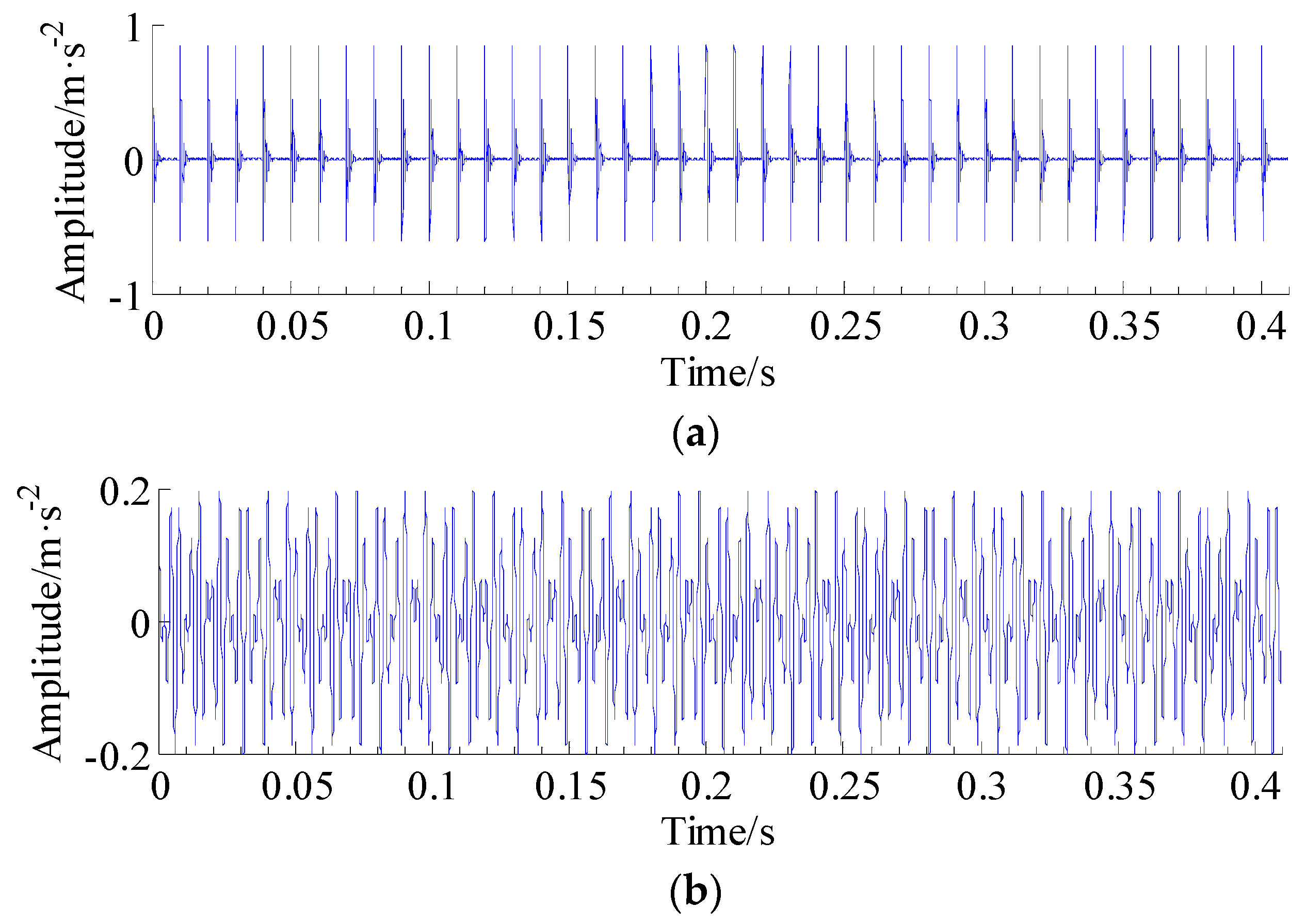
where A₀ = 1 m/s² is the intensity of the fault impulse impact, A₁ = 0.1 m/s² is the intensity of the systematic vibration signal, and the damping ratio is a = 0.1; in addition, f_n = 2000 Hz represents the natural frequency of excited structure, the length of vibration signal is N = 8192, the rotating frequencies are f₁ = 280 Hz and f₂ = 400 Hz, and the sampling frequency f_s = 20 KHz. Additionally, in this simulated case, the additive white noise x₃(t) with SDs sigma = 0.5, sigma = 0.7, and sigma = 0.9 are respectively added to the simulated signal, in order to test the noise tolerance of the proposed ACPR method. Therefore, it can be calculated that the gear fault frequency is 100 Hz (because the repetition interval T = 0.01, the sampling point of a single period is NT = round(fs*T), and the sampling time series is t₀ = (0:NT-1)/fs; therefore, the resonant frequency is 100 Hz). Figure 1a,b depict the obtained periodical impulse of the gear fault and natural modulated signal, respectively.

As a benchmark approach for gearbox fault detection, the Hilbert envelope spectrum has been effectively applied to fault diagnosis of rotating machinery, such as gears and rolling bearings. In this section, comparisons are made between the raw envelope spectrum method and envelope spectrums based on the proposed ACPR, on nonconvex penalty regularization (NCPR), and on the LFLO method, by analyzing simulated signals. In order to compare the diagnosis effect of the ACPR, NCPR, and LFLO methods, the evaluating parameters below are considered in

Table 2. Parameter settings of the proposed asymmetric convex penalty regularization (ACPR) method for gear fault detection.

Regularization Parameter λ0	Regularization Parameter λ1	Regularization Parameter λ2	M-Term	Iteration Times
λ0 = 0.35	λ1 =1.125	λ2 = 0.35	2	50

. Here, according to Equation (44), we will take the constant parameters to be β₀ = 0.7 and γ = 7.5. The parameters of the proposed ACPR can be obtained as follows: the standard deviation σ = 0.5, regularization term parameters λ₀ = 0.7 × 0.5 = 0.35, λ₁ = 7.5 × (1 − 0.7) × 0.5 = 1.125, and λ₂ = 0.7 × 0.5 = 0.35.

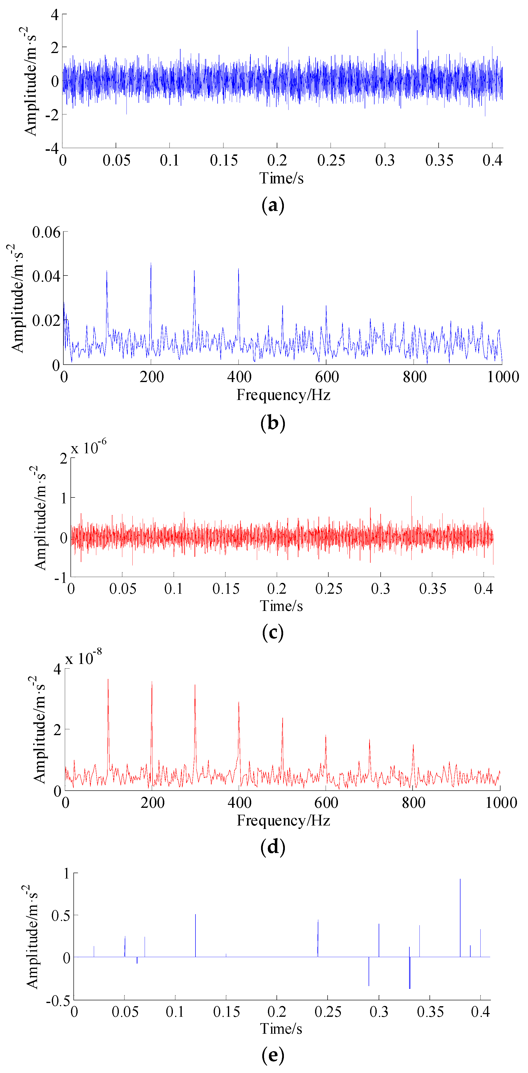
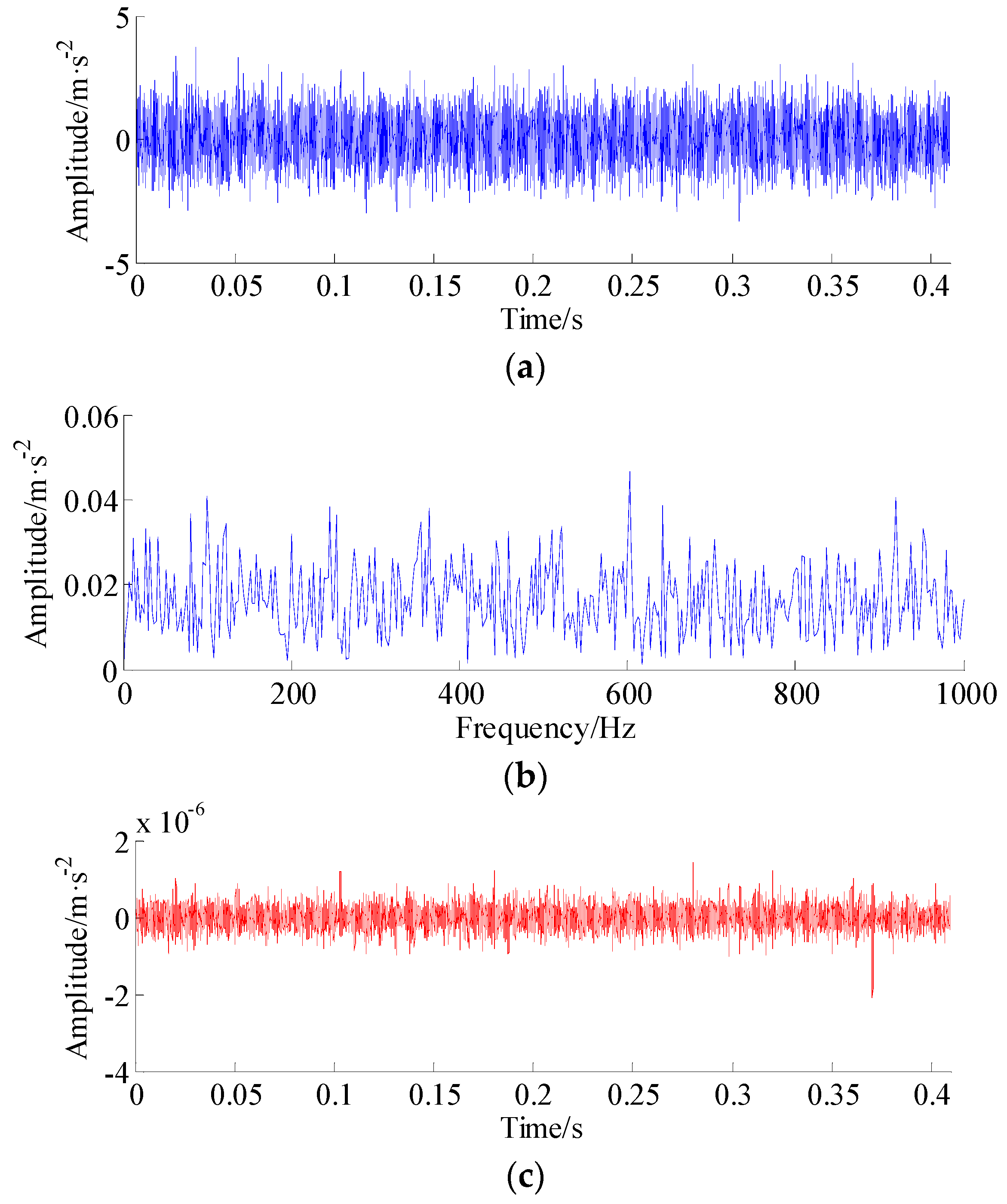
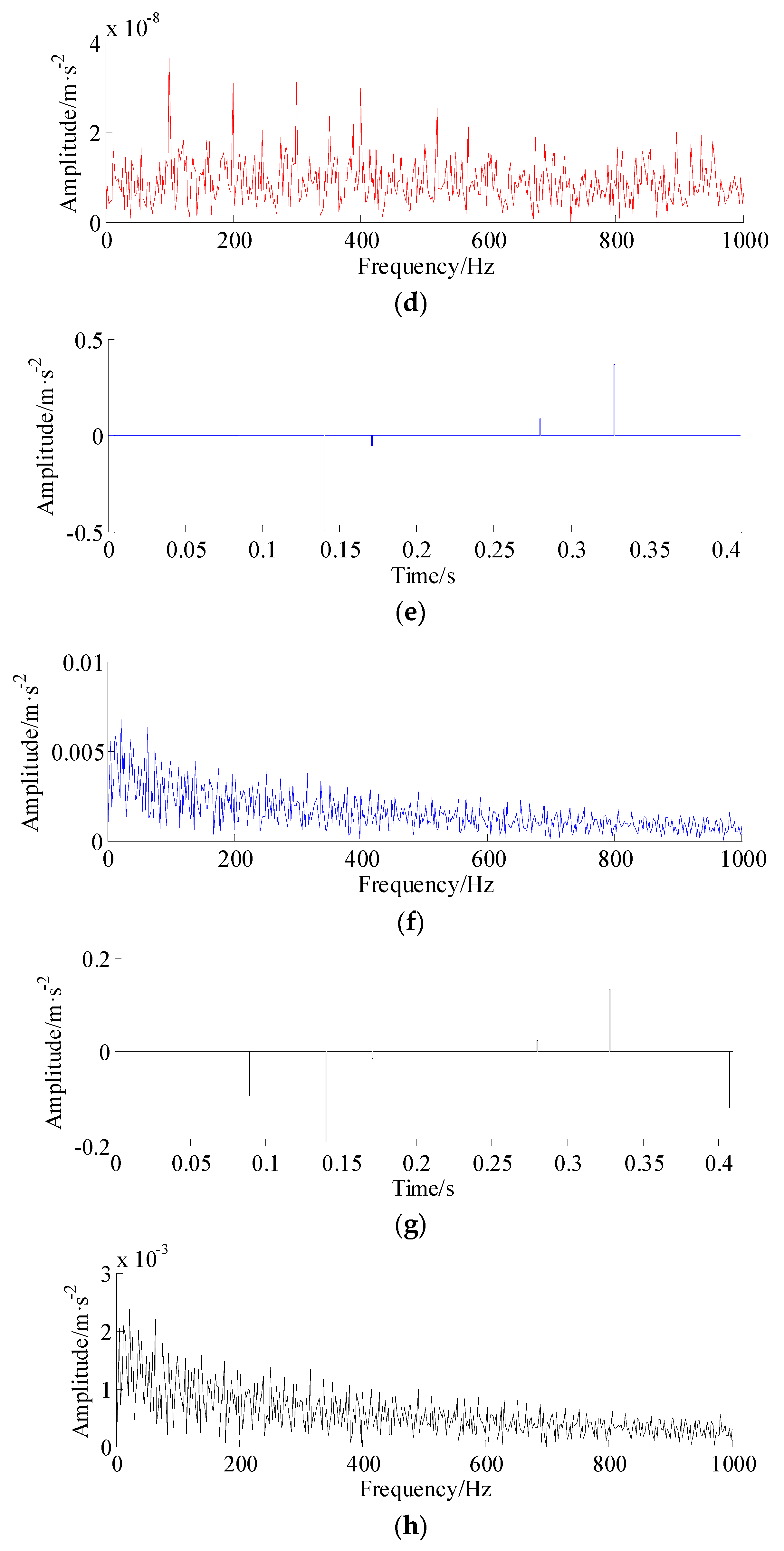
The simulated synthetic signal under noise a standard deviation sigma of 0.5, obtained from Equation (47), is shown in Figure 2a. From Figure 2a, it can be seen that the periodic impulses are completely buried in background noise. The Hilbert envelope spectrum of the raw synthetic signal is illustrated in Figure 2b, in which the fault frequencies 100 Hz and 200 Hz can be recognized from the envelope spectrum; however, those frequencies are clouded by the interference components. The resulting fault signal extracted through ACPR and its envelope spectrums are depicted in Figure 2c,d, revealing frequency information related to faults. Meanwhile, the resulting impulses components extracted through NCPR and LFLO and their envelope spectrums are exhibited in Figure 2e–h, respectively. As observed, in the case of SD = 0.5, all these results proved that the above three approaches can provide excellent performance in extracting the fault information, in contrast to the results from direct envelope spectrum analysis.

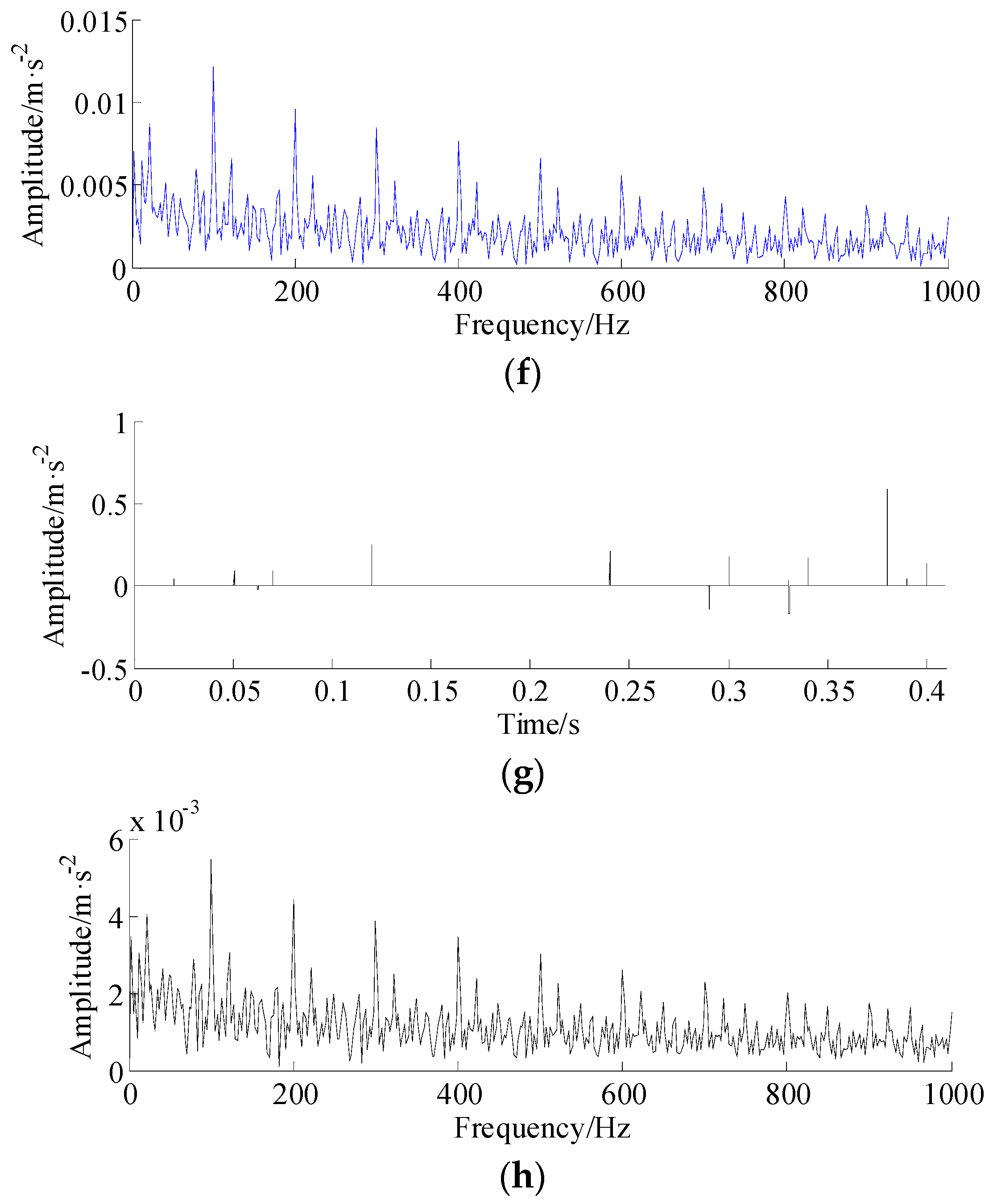
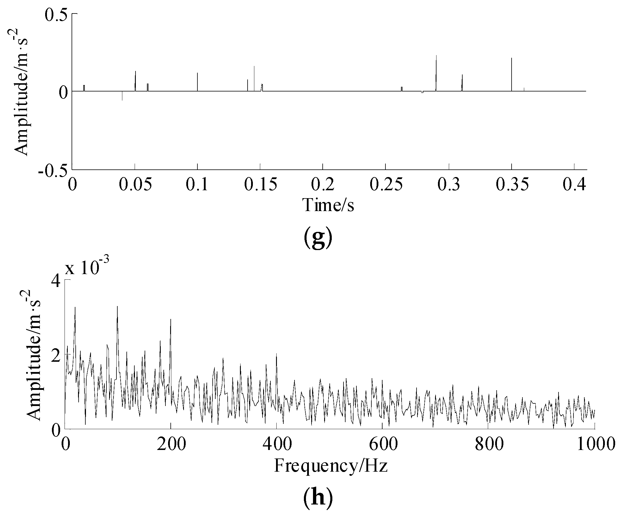
Next, with the purpose of testifying to the noise tolerance performance of the proposed ACPR, the vibration signals with different standard deviations (i.e., 0.7 and 0.9) are simulated and compared. The NCPR and LFLO methods are also used to process the simulated heavy noisy vibration signals, for comparison. The extraction results with different methods are illustrated in Figure 3 and Figure 4, respectively. As shown in Figure 3e,g and Figure 4e,g, most of noise harmonic interferences are removed; meanwhile, the energy of the useful fault periodic impulses is also reduced dramatically. It can be seen that, with the standard deviations (SD) of sigma increasing, the characteristic frequencies and their harmonic components cannot be accurately and clearly extracted by the NCPR and LFLO methods. Hence, the NCPR and LFLO methods are no longer effective for such a signal. Thankfully, the proposed ACPR is an appealing solution for the problem. It can be concluded that for the extraction results shown in Figure 3b–d and Figure 4b–d, the ACPR method is superior to the NCPR and LFLO methods in terms of increasing noise.

Table 3. The running time of the proposed algorithm and benchmarking methods.

Noise Standard Deviation	ACPR Algorithm	NCPR Algorithm	LFLO Algorithm
sigma = 0.5	0.288113 s	0.05391 s	0.000486 s
sigma = 0.7	0.283184 s	0.073986	0.000743 s
sigma = 0.9	0.308288 s	0.052860 s	0.000524 s

shows the running time of the proposed ACPR algorithm and other benchmarking methods. In this work, the simulation and experimental data were carried out by MATLAB, on a computer with Windows 10, quad-core processors at 2.9 GHz CPU, and 16 GB RAM.

In conclusion, when applied to the noisy signals, the proposed ACPR is more stable with regards to noise perturbation than the other two methods, at least when the noise standard deviation equals 0.7 and 0.9.

5. Experimental Validation

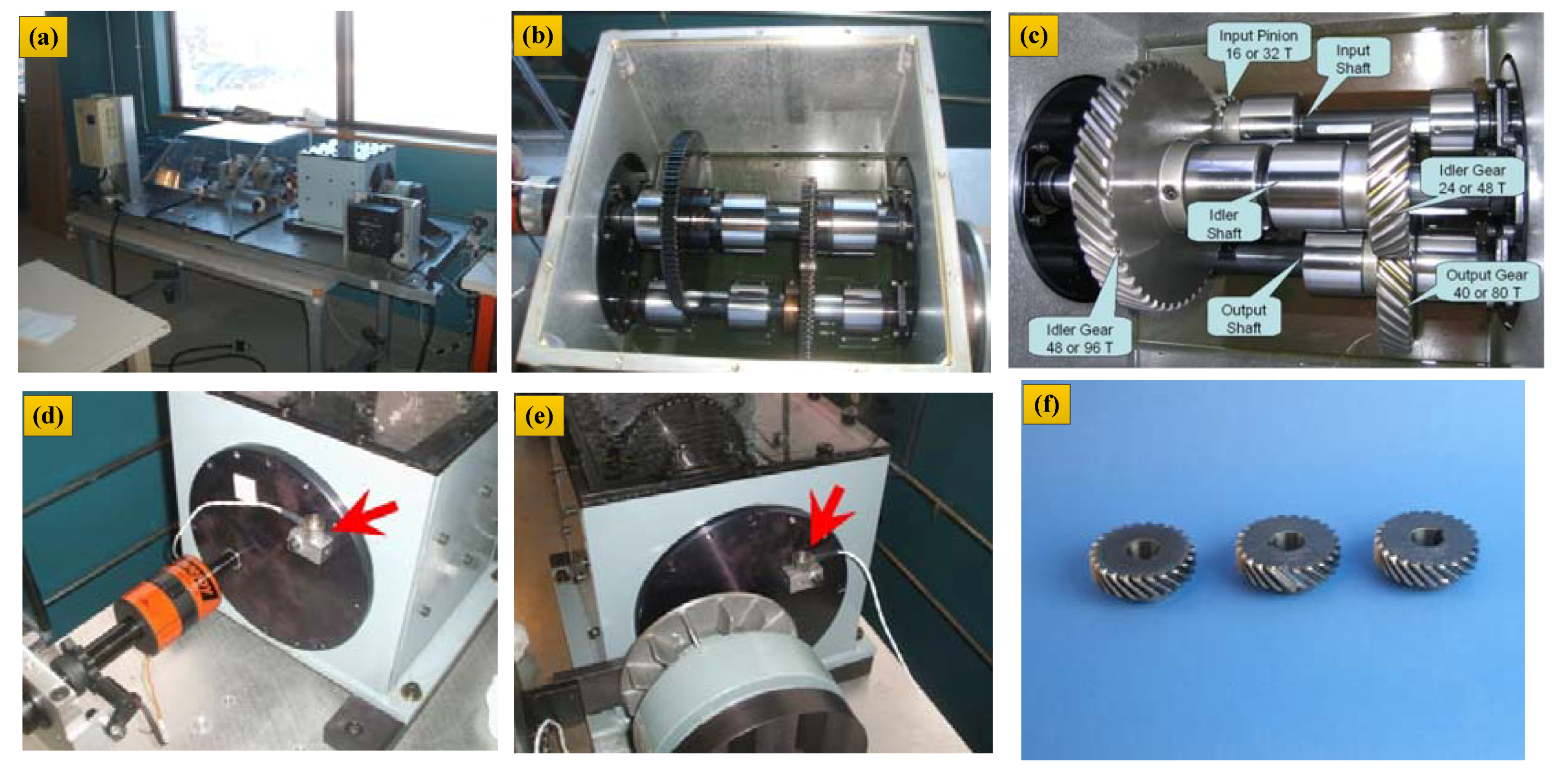
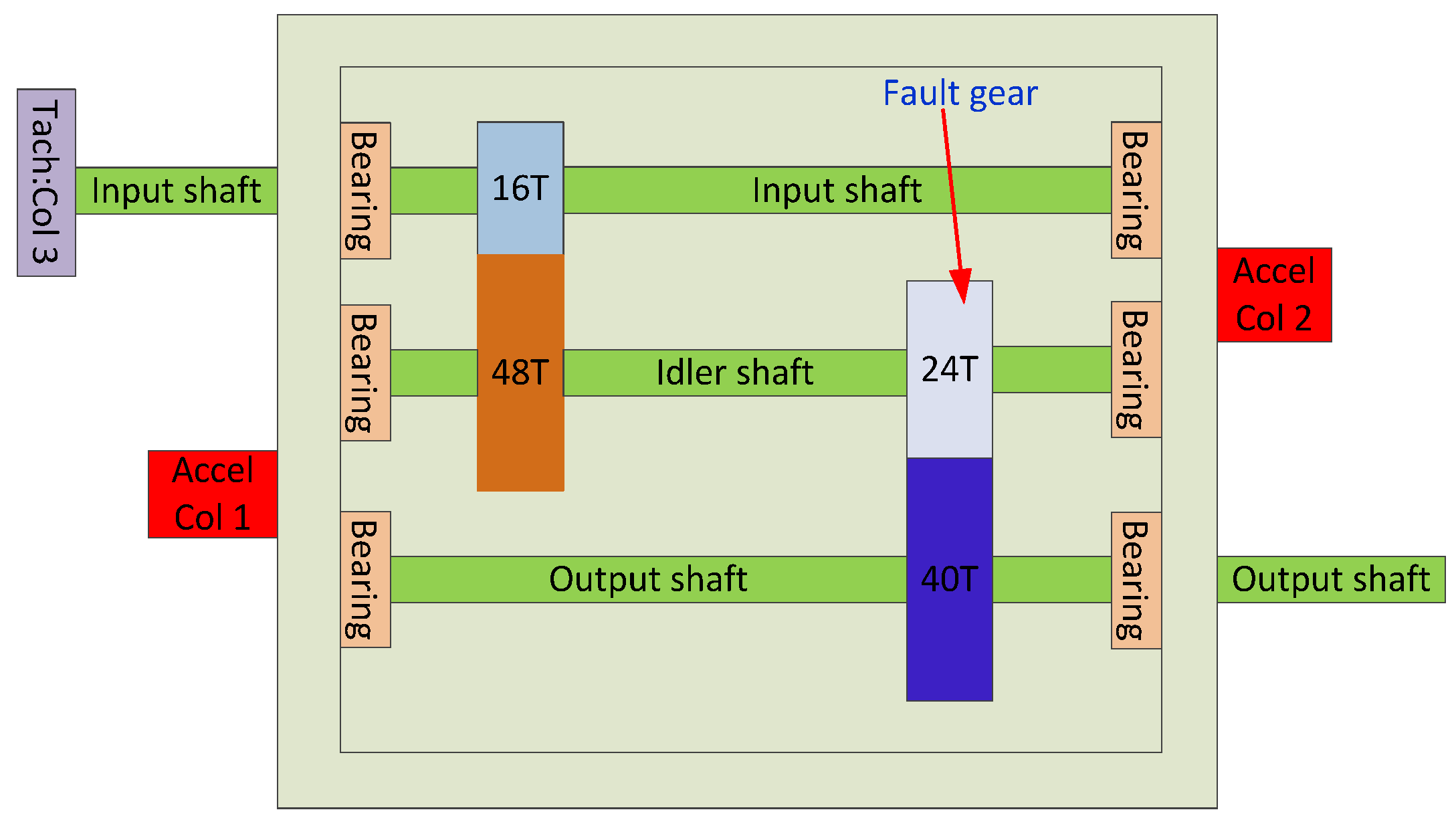
The experimental vibration data were collected via a two-class standard cylinder spur gear reducer [49,50]. The gearbox consists of an input shaft, an idler shaft, and an output shaft. The physical experimental rig and schematic diagram of the gearbox are shown in Figure 5 and Figure 6, respectively. There are 16 and 40 teeth of helical gear in the input and output shafts, respectively, and the two gears on the idler shaft have 48 teeth and 24 teeth. The first- and second-stage reduction gear ratios are 1.5 and 1.667, respectively. In this experiment, two triaxial accelerometers with three channels were mounted to the housing with magnetic bases, near the idler shaft (see Figure 5d,e), and the acquisition system was Endevco with 10 mv/g. An artificial fault (chipping failure with a small area) was produced on the tooth of a helical gear (i.e., 24 teeth in the idler shaft), and the vibration signal was picked up from the bearing pedestal with a sample frequency of 66.667 kHz. The shaft rotational speed was 2400 rpm (i.e., 40 Hz) with a low load, the sampling time was set to 4 seconds, and the characteristic defect frequency was 13.33 Hz (40 Hz × 16/48 = 13.33 Hz). It should be pointed out that the collected signals were not pre-filtered, and hence contains many interference factors and heavy background noise, which render more challenges for the implementation of weak fault detection.

More details about the experimental description and experiment parameters can be found at the website [49].

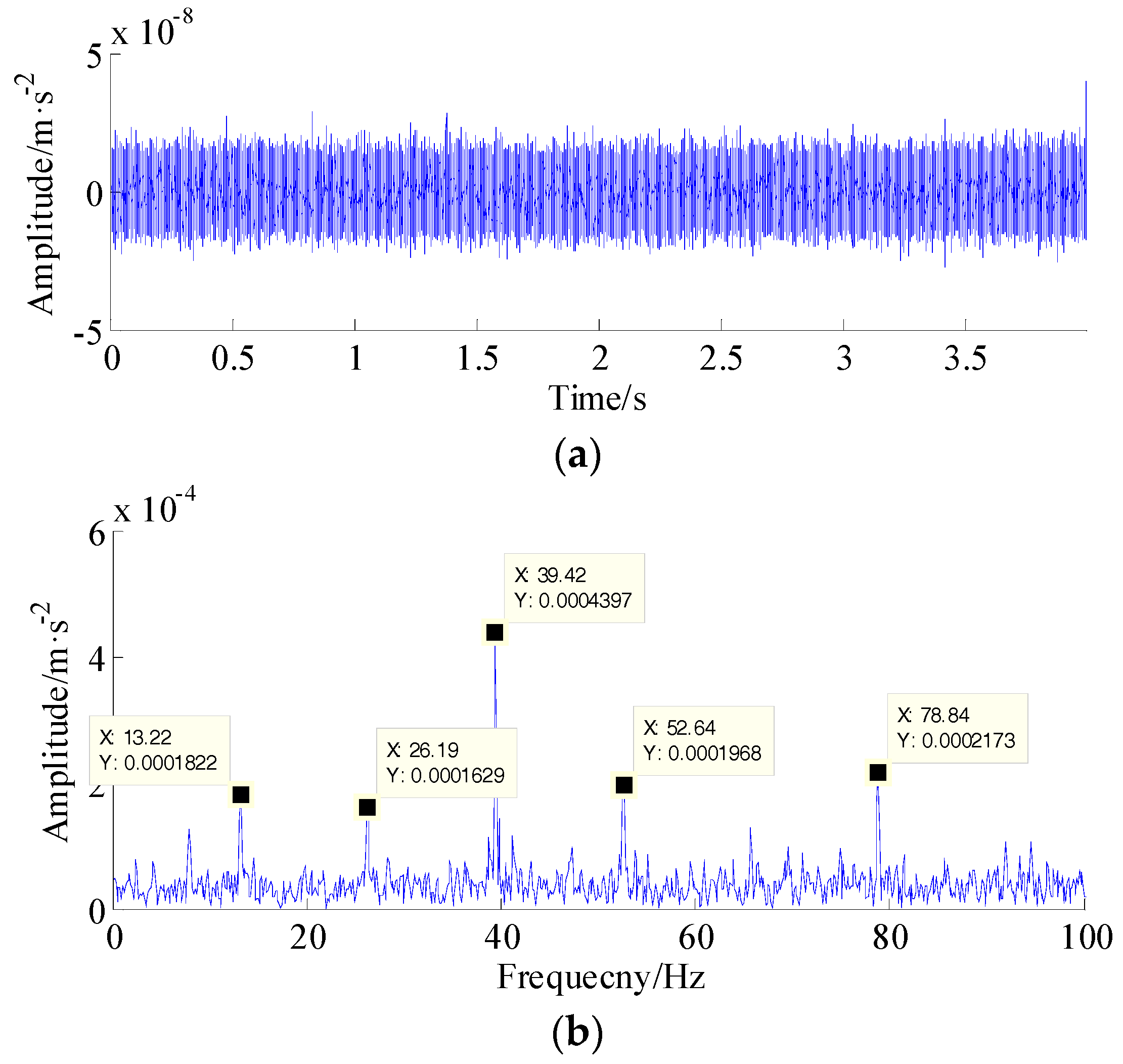
The raw vibration signal, (here in order to get a more complex vibration signal, a Gaussian white noise with amplitude sigma = 0.04 was added to the original signals) with a length of 4 s, is shown in Figure 7a, in which the periodic impulsive symptoms cannot be unraveled due to high level of noise and harmonic interference. Furthermore, no sign of the gear fault is revealed by its Hilbert envelope demodulation shown in Figure 7b—that is, the weak gear chipping characteristic frequency is completely submerged in the strong noise interference. Thus, an advanced signal processing method for weak fault detection should be developed.

The proposed ACPR method was adopted to process the raw vibration signal for the detected feature information. Since the standard deviation(SD)of the background noise was unknown, it could be calculated by the equation $\stackrel{\wedge }{\sigma }=MAD(y)/0.6745=0.0409$. Therefore, the related parameter specification for the ACPR approach is summarized in

Table 4. Parameter settings of the proposed ACPR method for gear fault detection.

Regularization Parameter λ0	Regularization Parameter λ1	Regularization Parameter λ2	M-Term	Iteration Times
λ0 = 0.02863	λ1 = 0.09203	λ2 = 0.02863	2	50

. Figure 8 depicts the extracted fault signal and its envelope spectrum. Compared with the original envelope spectrum shown in Figure 7b, it can be clearly seen that the gear chipping characteristic frequency was 13.22 Hz (close to the theoretical fault frequency of gear chipping, which was 13.33 Hz), and its higher orders (2f, 3f, 4f, and 5f) were obvious and had a satisfying distribution pattern. Therefore, it can be concluded that a localized fault exists on the helical gear with 24 teeth in the idler shaft.

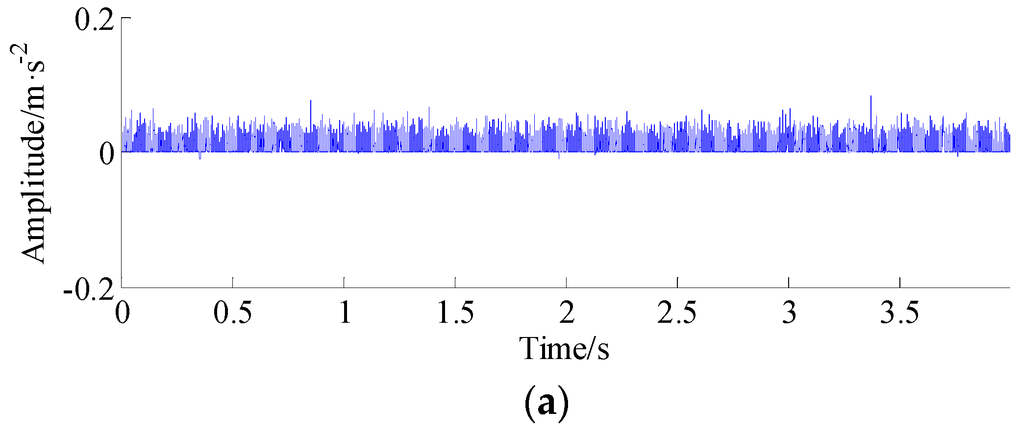
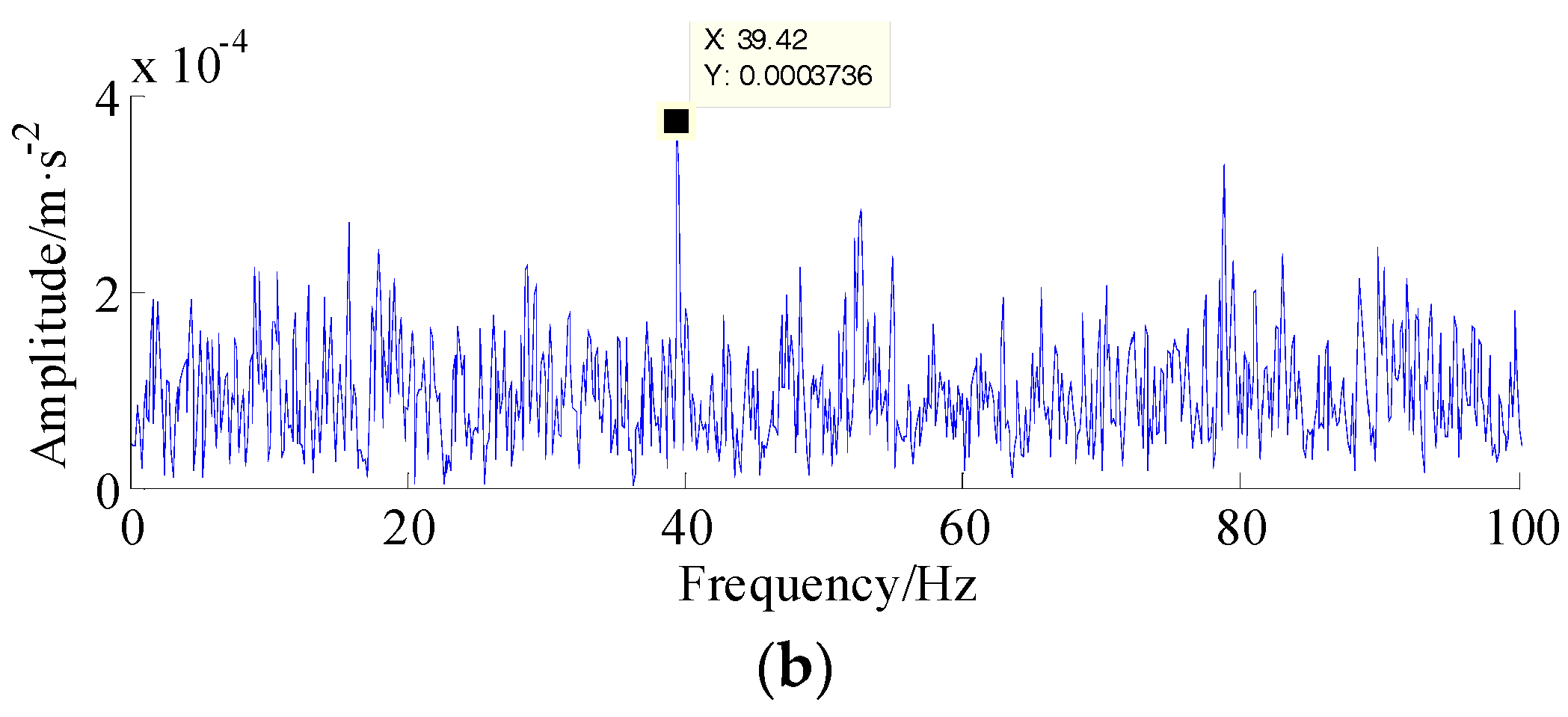
For the sake of comparing the diagnosis results obtained by the NCPR and LFLO methods, the parameters like regularization coefficients and penalty parameters were also calculated. The parameters of the algorithm are also given in Table 4. The detected fault components and related spectrum by the NCPR and LFLO methods are demonstrated in Figure 9 and Figure 10. From Figure 9 and Figure 10, however, only one higher order line (39.42 Hz) associated with the gear chipping fault can be observed, so the fundamental frequency of failure of 13.33 Hz cannot be reliably identified. This may because of the fact that the gear chipping fault, in this case, was quite weak and was submerged by strong noise. Therefore, it can be verified that the proposed ACPR method has an excellent performance with regards to recognizing the fault information of weak gearbox failure, in comparison with the NCPR and LFLO methods.

6. Conclusions

Aiming at the issue of estimating the sparse low-rank matrix (i.e., the weak fault signal) from its noise observation, this paper proposes a novel weak fault feature extraction approach for a gearbox, combining majorization–minimization (MM) and asymmetric convex penalty regularization (ACPR) algorithms. In this work, the observed noisy signal was modeled as the sum of the fault’s transient impulses, the systematic natural vibration signal, and the additive noise; thus, the ill-posed problem of sparse representation was translated into a regularization inverse problem. The proposed objective function better estimates sparse low-rank matrices (SLRM) than the nonconvex and convex methods, which utilize the sum of the signal-fidelity term and the two parameterized penalty terms.

In terms of an algorithm solution, the asymmetric penalty function was established on the basis of the L1-norm model and simple quadratic equation forms, and a symmetric penalty function was established on the basis of the L1-norm model, respectively. Then, the majorizers of the symmetric and asymmetric functions were calculated via the majorization–minimization (MM) algorithm. Afterward, the efficient iterative algorithm was derived by the MM algorithm. Meanwhile, we show how to set the model parameters of the proposed objective cost function (OCF), in order to ensure that the objective function is strictly convex. Finally, the effectiveness of the proposed ACPR method is demonstrated by the simulation signal and practical gearbox fault data, compared with two state-of-art methods, especially for the measured signal with heavy background noise. specifically, the gear chipping characteristic frequency 13.22 Hz and its harmonic (2f, 3f, 4f and 5f) can be detected obviously. The diagnosis results show that the fault frequency and its harmonics could be detected clearly by the proposed method.

The proposed approach has great potential for online or offline detection for gearboxes, especially in the early stages of failure or when the background noise is heavy and uncorrelated interference is very strong. The proposed ACPR approach uses symmetric and asymmetric penalty functions to promote the positivity of the estimated fault signal; however, it should be noted that the periodic transient characteristics of fault impulses cannot be revealed by the current proposed methodology. Hence, future work will focus on formulating an improved algorithm to address this issue, which makes periodic transient impulses as similar to the signal’s physical structure as possible.

For the applicability of the proposed algorithm, this algorithm might be applied to other rotating machinery, such as a rolling bearing or rotor, and even mechanical processing (e.g., turning chatter, milling chatter, tool wear etc.).

References

- Jing, L.Y.; Zhao, M.; Li, P.; Xu, X.Q. A convolutional neural network based feature learning and fault diagnosis method for the condition monitoring of gearbox. Measurement 2017, 111, 1–10. [Google Scholar] [CrossRef]
- Li, Y.B.; Li, G.Y.; Yang, Y.T.; Liang, X.H.; Xu, M.Q. A fault diagnosis scheme for planetary gearboxes using adaptive multi-scale morphology filter and modified hierarchical permutation entropy. Mech. Syst. Signal Process. 2018, 105, 319–337. [Google Scholar] [CrossRef]
- Kia, S.H.; Henao, H.; Capolino, G.A. Fault index statistical study for gear fault detection using stator current space vector analysis. IEEE Trans. Ind. Appl. 2016, 52, 781–4788. [Google Scholar] [CrossRef]
- Teng, W.; Ding, X.; Zhang, X.L.; Liu, Y.B.; Ma, Z.Y. Multi-fault detection and failure analysis of wind turbine gearbox using complex wavelet transform. Renew. Energy 2016, 93, 591–598. [Google Scholar] [CrossRef]
- Hemmati, F.; Orfali, W.; Gadala, M.S. Roller bearing acoustic signature extraction by wavelet packet transform, applications in fault detection and size estimation. Appl. Acoust. 2016, 104, 101–118. [Google Scholar] [CrossRef]
- Qu, J.X.; Zhang, Z.S.; Gong, T. A novel intelligent method for mechanical fault diagnosis based on dual-tree complex wavelet packet transform and multiple classifier fusion. Neurocomputing 2016, 171, 837–853. [Google Scholar] [CrossRef]
- Wang, L.H.; Zhao, X.P.; Wu, J.X.; Xie, Y.Y.; Zhang, Y.H. Motor fault diagnosis based on short-time Fourier transform and convolutional neural network. Chin. J. Mech. Eng. 2017, 30, 1357–1368. [Google Scholar] [CrossRef]
- Bouchikhi, E.H.E.; Choqueuse, V.; Benbouzid, M.E.H. Current frequency spectral subtraction and its contribution to induction machines bearings condition monitoring. IEEE Trans. Energy Convers. 2013, 28, 135–144. [Google Scholar] [CrossRef] [Green Version]
- Wang, H.C.; Chen, J.; Dong, G.M. Feature extraction of rolling bearing’s early weak fault based on EEMD and tunable Q-factor wavelet transform. Mech. Syst. Signal Process. 2014, 48, 103–119. [Google Scholar] [CrossRef]
- Li, Q.; Liang, S.Y. Bearing incipient fault diagnosis based upon maximal spectral kurtosis TQWT and group sparsity total variation de-noising approach. J. Vibroeng. 2018, 20, 1409–1425. [Google Scholar] [CrossRef]
- Li, R.Y.; He, D. Rotational machine health monitoring and fault detection using EMD-based acoustic emission feature quantification. IEEE Trans. Instrum. Meas. 2012, 61, 990–1001. [Google Scholar] [CrossRef]
- Yuan, J.; Ji, F.; Gao, Y.; Zhu, J.; Wei, C.J.; Zhou, Y. Integrated ensemble noise-reconstructed empirical mode decomposition for mechanical fault detection. Mech. Syst. Signal Process. 2018, 104, 323–346. [Google Scholar] [CrossRef]
- Wang, L.; Liu, Z.W.; Miao, Q.; Zhang, X. Time-frequency analysis based on ensemble local mean decomposition and fast kurtogram for rotating machinery fault diagnosis. Mech. Syst. Signal Process. 2018, 103, 60–75. [Google Scholar] [CrossRef]
- Li, Q.; Liang, S.Y.; Song, W.Q. Revision of bearing fault characteristic spectrum using LMD and interpolation correction algorithm. Procedia CIRP 2016, 56, 182–187. [Google Scholar] [CrossRef]
- Li, Z.X.; Jiang, Y.; Guo, Q.; Hu, C.; Peng, Z.X. Multi-dimensional variational mode decomposition for bearing-crack detection in wind turbines with large driving-speed variations. Renew. Energy 2018, 116, 55–73. [Google Scholar] [CrossRef]
- Li, Q.; Ji, X.; Liang, S.Y. Incipient fault feature extraction for rotating machinery based on improved AR-minimum entropy deconvolution combined with variational mode decomposition approach. Entropy 2017, 19, 7. [Google Scholar] [CrossRef]
- Zhang, R.; Tao, H.Y.; Wu, L.F.; Guan, Y. Transfer learning with neural networks for bearing fault diagnosis in changing working conditions. IEEE Access 2017, 5, 14347–14357. [Google Scholar] [CrossRef]
- Masud, A.A.; Albarracín, R.; Rey, J.A.A.; Sukki, F.M.; Illias, H.A.; Bani, N.A.; Munir, A.B. Artificial Neural Network Application for Partial Discharge Recognition: Survey and Future Directions. Energies 2016, 9, 574. [Google Scholar] [CrossRef]
- He, M.; He, D. Deep learning based approach for bearing fault diagnosis. IEEE Trans. Ind. Appl. 2017, 53, 3057–3065. [Google Scholar] [CrossRef]
- Jia, F.; Lei, Y.G.; Guo, L.; Lin, J.; Xing, S.B. A neural network constructed by deep learning technique and its application to intelligent fault diagnosis of machines. Neurocomputing 2018, 272, 619–628. [Google Scholar] [CrossRef]
- Li, Q.; Liang, S.Y. Multiple faults detection for rotating machinery based on Bi-component sparse low-rank matrix separation approach. IEEE Access 2018, 6, 20242–20254. [Google Scholar] [CrossRef]
- Tang, H.F.; Chen, J.; Dong, G.M. Sparse representation based latent components analysis for machinery weak fault detection. Mech. Syst. Signal Process. 2014, 46, 373–388. [Google Scholar] [CrossRef]
- Zhou, H.T.; Chen, J.; Dong, G.M.; Wang, R. Detection and diagnosis of bearing faults using shift-invariant dictionary learning and hidden Markov model. Mech. Syst. Signal Process. 2016, 72–73, 65–79. [Google Scholar] [CrossRef]
- Yang, B.Y.; Liu, R.N.; Chen, X.F. Fault diagnosis for a wind turbine generator bearing via sparse representation and shift-invariant K-SVD. IEEE Trans. Ind. Inform. 2017, 13, 1321–1331. [Google Scholar] [CrossRef]
- Feng, Z.P.; Liang, M. Complex signal analysis for planetary gearbox fault diagnosis via shift invariant dictionary learning. Measurement 2016, 90, 382–395. [Google Scholar] [CrossRef]
- Qin, Y. A new family of model-based impulsive wavelets and their sparse representation for rolling bearing fault diagnosis. IEEE Trans. Ind. Electron. 2018, 65, 2716–2726. [Google Scholar] [CrossRef]
- Cui, L.L.; Wang, J.; Lee, S. Matching pursuit of an adaptive impulse dictionary for bearing fault diagnosis. J. Sound Vib. 2014, 333, 2840–2862. [Google Scholar] [CrossRef]
- Cui, L.L.; Gong, X.Y.; Zhang, J.Y.; Wang, H.Q. Double-dictionary matching pursuit for fault extent evaluation of rolling bearing based on the Lempel-Ziv complexity. J. Sound Vib. 2016, 385, 372–388. [Google Scholar] [CrossRef]
- Cui, L.L.; Wu, N.; Ma, C.Q.; Wang, H.Q. Quantitative fault analysis of roller bearings based on a novel matching pursuit method with a new step-impulse dictionary. Mech. Syst. Signal Process. 2016, 68–69, 34–43. [Google Scholar] [CrossRef]
- Ding, X.X.; He, Q.B. Time-frequency manifold sparse reconstruction: A novel method for bearing fault feature extraction. Mech. Syst. Signal Process. 2016, 80, 392–413. [Google Scholar] [CrossRef]
- Li, Q.; Liang, S.Y. Incipient fault diagnosis of rolling bearings based on impulse-step impact dictionary and re-weighted minimizing nonconvex penalty Lq regular technique. Entropy 2017, 19, 8. [Google Scholar] [CrossRef]
- Ding, Y.; He, W.P.; Chen, B.Q.; Zi, Y.Y.; Selesnick, I.W. Detection of faults in rotating machinery using periodic time-frequency sparsity. J. Sound Vib. 2016, 382, 357–378. [Google Scholar] [CrossRef] [Green Version]
- He, W.P.; Ding, Y.; Zi, Y.Y.; Selesnick, I.W. Sparsity-based algorithm for detecting faults in rotating machines. Mech. Syst. Signal Process. 2016, 72–73, 46–64. [Google Scholar] [CrossRef]
- He, W.P.; Ding, Y.; Zi, Y.Y.; Selesnick, I.W. Repetitive transients extraction algorithm for detecting bearing faults. Mech. Syst. Signal Process. 2017, 84, 227–244. [Google Scholar] [CrossRef] [Green Version]
- Zhang, H.; Chen, X.F.; Du, Z.H.; Li, X.; Yan, R.Q. Nonlocal sparse model with adaptive structural clustering for feature extraction of aero-engine bearings. J. Sound Vib. 2016, 368, 223–248. [Google Scholar] [CrossRef]
- Du, Z.H.; Chen, X.F.; Zhang, H.; Yang, B.Y.; Zhai, Z.; Yan, R.Q. Weighted low-rank sparse model via nuclear norm minimization for bearing fault detection. J. Sound Vib. 2017, 400, 270–287. [Google Scholar] [CrossRef]
- Mourad, N.; Reilly, J.P.; Kirubarajan, T. Majorization minimization for blind source separation of sparse sources. Signal Process. 2017, 131, 120–133. [Google Scholar] [CrossRef]
- Qiu, T.Y.; Palomar, D.P. Undersampled sparse phase retrieval via majorization minimization. IEEE trans. Signal Process. 2017, 65, 5957–5969. [Google Scholar] [CrossRef]
- Ndoye, M.; Anderson, J.M.M.; Greene, D.J. An MM-based algorithm for ℓ1-regularized least-squares estimation with an application to ground penetrating radar image reconstruction. IEEE Trans. Image Process. 2016, 25, 2206–2221. [Google Scholar] [CrossRef] [PubMed]
- Donoho, D.L.; Elad, M.; Temlyakov, V.N. Stable recovery of sparse overcomplete representations in the presence of noise. IEEE Trans. Inform. Theory 2006, 52, 6–18. [Google Scholar] [CrossRef] [Green Version]
- Donoho, D.L. Compressed sensing. IEEE Trans. Inform. Theory 2006, 52, 1289–1306. [Google Scholar] [CrossRef]
- Donoho, D.L.; Tsaig, Y. Fast solution of ℓ1-norm minimization problems when the solution may be sparse. IEEE Trans. Inform. Theory 2008, 54, 4789–4812. [Google Scholar] [CrossRef]
- Donoho, D.L. De-noising by soft-thresholding. IEEE Trans. Inf. Theory 1995, 41, 613–627. [Google Scholar] [CrossRef] [Green Version]
- Selesnick, I.W. Total variation denoising via the Moreau envelope. IEEE Signal Process. Lett. 2017, 24, 216–220. [Google Scholar] [CrossRef]
- Selesnick, I.W.; Parekh, A.; Bayram, I. Convex 1-D total variation denoising with non-convex regularization. IEEE Signal Process. Lett. 2015, 22, 141–144. [Google Scholar] [CrossRef]
- Selesnick, I.W.; Graber, H.L.; Pfeil, D.S.; Barbour, R.L. Simultaneous low-pass filtering and total variation denoising. IEEE Trans. Signal Process. 2014, 62, 1109–1124. [Google Scholar] [CrossRef]
- Ning, X.R.; Selesnick, I.W.; Duval, L. Chromatogram baseline estimation and denoising using sparsity (BEADS). Chemom. Intell. Lab. 2014, 139, 156–167. [Google Scholar] [CrossRef]
- Donoho, D.L.; Johnstone, I.M. Ideal spatial adaptation by wavelet shrinkage. Biometrika 1993, 81, 425–455. [Google Scholar] [CrossRef]
- Annual Conference of the Prognostics and Health Management Society 2009. Available online: https://www.phmsociety.org/events/conference/phm/09 (accessed on 5 June 2018).
- Atat, H.A.; Siegel, D.; Lee, J. A systematic methodology for gearbox health assessment and fault classification. Int. J. Progn. Health Manag. 2011, 2, 1. [Google Scholar]
Figure 1.
Simulated synthetic signal. (a) Faulty periodical transient impulses of a gearbox; and (b) the systematic natural modulated signal.
Figure 2.
A simulated synthetic signal, its detected impulses, and its envelope spectrum, using the proposed non-convex penalty regularization and L1-norm fused lasso optimization (LFLO) method, when noise standard deviation is 0.5. (a) Simulated synthetic signal; (b) envelope spectrum of the simulated synthetic signal; (c) detected impulses using the proposed ACPR method; (d) envelope spectrum of detected impulses using proposed ACPR method; (e) detected impulses using the nonconvex penalty regularization (NCPR) method; (f) envelope spectrum of detected impulses using the NCPR method; (g) detected impulses using the LFLO method; (h) envelope spectrum of detected impulses using the LFLO method.
Figure 3.
A simulated synthetic signal, its detected impulses, and its envelope spectrum, using the proposed non-convex penalty regularization and LFLO methods, when noise standard deviation sigma is 0.7. (a) Simulated synthetic signal; (b) envelope spectrum of simulated synthetic signal; (c) detected impulses using the proposed ACPR method; (d) envelope spectrum of detected impulses using the proposed ACPR method; (e) detected impulses using the NCPR method; (f) envelope spectrum of detected impulses using the NCPR method; (g) detected impulses using the LFLO method; and (h) envelope spectrum of detected impulses using the LFLO method.
Figure 4.
The simulated synthetic signal, its detected impulses, and its envelope spectrum, using the proposed non-convex penalty regularization and LFLO methods, when the noise standard deviation sigma is 0.9. (a) Simulated synthetic signal; (b) envelope spectrum of the simulated synthetic signal; (c) detected impulses using the proposed ACPR method; (d) envelope spectrum of detected impulses using the proposed ACPR method; (e) detected impulses using the NCPR method; (f) envelope spectrum of detected impulses using the NCPR method; (g) detected impulses using the LFLO method; and (h) envelope spectrum of detected impulses using the LFLO method.
Figure 5.
Experimental setup for the gearbox multiple faults. (a) Overview of the experimental apparatus; (b) the internal structure the gearbox; (c) the internal structure of the gear meshing; (d) the installation location of input shaft accelerometer; (e) the installation location of the output shaft accelerometer; and (f) the gears with failure [49,50].
Figure 7.
The raw vibration signal and its Hilbert envelope spectrum. (a) The raw vibration signal and (b) the Hilbert envelope spectrum of that raw vibration signal.
Figure 8.
The fault information extracted through the proposed approach. (a) The time-domain waveform of the extracted fault signal and (b) the envelope spectrum of the extracted fault signal.
Figure 9.
The fault information extracted through the NCPR approach. (a) The time-domain waveform of extracted fault signal and (b) the envelope spectrum of the extracted fault signal.
Figure 10.
The fault information extracted through the LFLO approach. (a) The time-domain waveform of the extracted fault signal and (b) the envelope spectrum of the extracted fault signal.