Article

A Hybrid Fuzzy Inference System Based on Dispersion Model for Quantitative Environmental Health Impact Assessment of Urban Transportation Planning

by
Behnam Tashayo
1,*,
Abbas Alimohammadi
1,2 and
Mohammad Sharif
1
1
Department of Geospatial Information Systems, Faculty of Geodesy and Geomatics Engineering, K. N. Toosi University of Technology, Tehran 19967 15433, Iran
2
Center of Excellence in Geospatial Information Technology, Faculty of Geodesy and Geomatics Engineering, K. N. Toosi University of Technology, Tehran 19967 15433, Iran
*
Author to whom correspondence should be addressed.
Sustainability 2017, 9(1), 134; https://doi.org/10.3390/su9010134
Submission received: 27 November 2016 / Revised: 3 January 2017 / Accepted: 13 January 2017 / Published: 18 January 2017

Abstract

:
Characterizing the spatial variation of traffic-related air pollution has been and is a long-standing challenge in quantitative environmental health impact assessment of urban transportation planning. Advanced approaches are required for modeling complex relationships among traffic, air pollution, and adverse health outcomes by considering uncertainties in the available data. A new hybrid fuzzy model is developed and implemented through hierarchical fuzzy inference system (HFIS). This model is integrated with a dispersion model in order to model the effect of transportation system on the PM2.5 concentration. An improved health metric is developed as well based on a HFIS to model the impact of traffic-related PM2.5 on health. Two solutions are applied to improve the performance of both the models: the topologies of HFISs are selected according to the problem and used variables, membership functions, and rule set are determined through learning in a simultaneous manner. The capabilities of this proposed approach is examined by assessing the impacts of three traffic scenarios involved in air pollution in the city of Isfahan, Iran, and the model accuracy compared to the results of available models from literature. The advantages here are modeling the spatial variation of PM2.5 with high resolution, appropriate processing requirements, and considering the interaction between emissions and meteorological processes. These models are capable of using the available qualitative and uncertain data. These models are of appropriate accuracy, and can provide better understanding of the phenomena in addition to assess the impact of each parameter for the planners.

1. Introduction

Over the last two decades, the use of health impact assessment for incorporating the issue of health in planning and decision-making, has been and is on an increase [1]. According to WHO, health impact assessment is a method to assess the health impacts of policies, plans, and projects in diverse economic sectors, through quantitative and qualitative techniques. The policy, plan, or project is briefly named a scenario hereafter, most of which affect the health through their effect on environmental health indices. The impact assessment (IA) methods that evaluate the impact of a scenario on environmental indices, followed by, the impact of changes in environmental indices on health, are known as the environmental health impact assessment (EHIA) [2]. Due to the widespread effects of transportation on health, the major focus of EHIA is on transportation [3,4]. Most of these EHIA assess the air quality impacts, mainly due to the availability of models, essential information, and the extent of air quality impacts on health [5]. An efficient EHIA must be capable of compute the impacts of various scenarios and prioritize them [6]. Development of such capabilities requires quantitative methods [7,8,9]. The quantitative methods typically determine the impact by estimating the number of occurred or avoided cases as a result of change in pollutant concentration.
In general, quantitative EHIA for air quality consists of two stages: (1) determining the pollutant concentration (e.g., PM2.5); and (2) computing the impact of human exposure to pollution. Ideally, quantitative EHIA could be achieved by monitoring the population exposed to air population, which in fact is impossible due to cost and time restrictions especially at urban scale [10]. The initial studies concerning the effect of air pollution on health are run through urban monitoring stations to estimate the concentration of pollutants [11]. These stations only estimate large-scale spatial variations. During the past decade, some studies have proven significant and small-scale pollutants variability in urban regions [12]. The differences of some pollutants concentrations (e.g., PM2.5) in intra city are similar to that of the inter cities [13]. Consequently, quantitative assessment of exposure requires the modeling of pollutant concentration with appropriate spatial resolution [14,15]. Dispersion and land use regression (LUR) models are applied to improve the spatial resolution of pollutant concentration [10,16,17].
In general, to develop regression models, the data derived from air pollution monitoring stations are applied. Due to inefficient number of monitoring stations, located in certain places in a given city, occurrence of substantial errors in regression models in regions where the urban pattern is different from the location of urban monitoring stations is inevitable [18,19]. The LUR models fail to model small-scale pollutant variability due to interactions between emission sources and meteorological processes [20,21]. These limitations make the regression models unable to determine the true contribution of transportation on air pollution [22]. By comparing the dispersion models to the regression models, the first has greater spatial and temporal resolutions. Dispersion models make it possible to assess the impact of a particular source of pollution on air pollution, and health thereof in an efficient manner. According to Brauer et al. (2008) and Michanowicz (2015), dispersion models require numerous high-density data including temporally and spatially separated emissions data and intensive computation, which has led to their rare adoption in epidemiological and impact assessment studies [23,24]. Unlike dispersion models regression models, require fewer inputs and computation [25], therefore, they are widely used in epidemiological and impact assessment studies.
To overcome the drawbacks and take advantage of different modeling methods, especially for environmental health impact assessments, the integration of these models has become more common [24,26,27]. Most of the available studies apply dispersion model output as dependent variable in order to develop the landuse regression model [28,29,30]. Adopting dispersion models for generating regression models can improve the spatial and temporal resolutions and increase the accuracy by incorporating source-meteorology interaction information [12,20,26]. Despite the advances made in modeling pollutants concentrations, a limited use of these models is reported for quantitative EHIA. Most of the applied practical EHIAs (75%) for air pollution are qualitative [31], indicating that conventional models are not capable to meet EHIAs requirements.
Numerous parameters are required to determine the PM2.5 concentration and to estimate the exposure impact in quantitative EHIA in transportation scenarios. These parameters are the results of various studies, modeling, and computation and consist of: traffic parameters, especially after the implementation of a scenario, are merely a result of traffic modeling; the parameters of meteorological data, which are associated with uncertainty; and the parameters of concentration-response coefficient and total adverse health outcome the derived from analysis of limited population. Accordingly, the abovementioned parameters are generally uncertain, diverse, descriptive, and heterogeneous [9,32,33,34]. Thus, a significant part of academic research focus on modeling uncertainty in IA [35,36].
Neither conventional dispersion models nor LUR are capable of considering the uncertainty of the parameters applied in EHIA. These models are not flexible to apply heterogeneous, descriptive, and uncertain data. The amount of required data together with considering their uncertainty and their computational mass are the major contributors to the practicality of air pollution prediction model and health metric [2,33,37,38]. Applying fuzzy inference systems in EHIA provide the possibility of establishing an appropriate model from the available heterogeneous, descriptive, and uncertain data. Moreover, the flexibility of such models in applying qualitative and quantitative data contributes to their practical state in different stages of planning and decision-making, like informing the decision makers, developing, assessing, and selecting the scenarios [39].
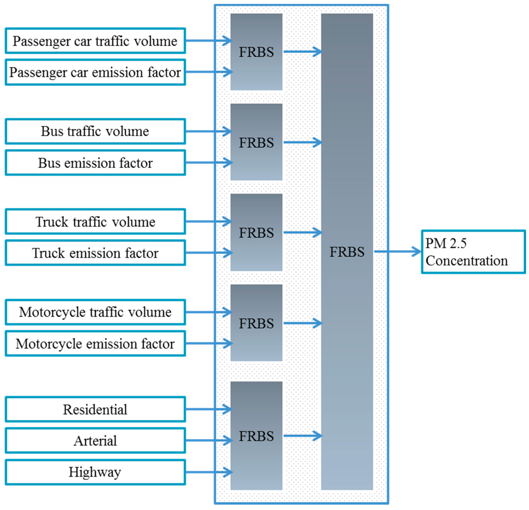
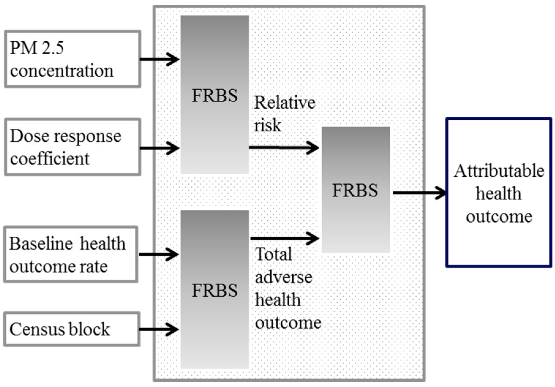
In this paper, a hybrid fuzzy model is proposed to quantitatively assess the environmental health impacts of transportation scenarios. In this model, the data from an air dispersion model are applied in establishing a hierarchical fuzzy inference system in order to determine the suspended particles concentration (i.e., PM2.5). In addition, another hierarchical fuzzy inference system is developed based on epidemiological evidence, applied in estimating the health outcome caused by PM2.5 concentration. Due to the nature of the EHIA, flexibility and performance constitute the core of developing such models. Linguistic modeling is applied to create the essential flexibility and hierarchical structure, and NSGA2 multi-objective optimization algorithm is applied to enhance the models’ performance. To evaluate these proposed models, three traffic scenarios are examined in the city of Isfahan, Iran.

2. Transportation and Air Pollution in the City of Isfahan

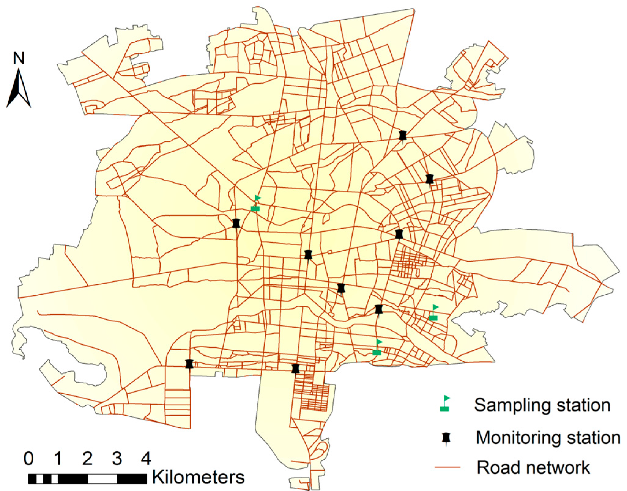
The city of Isfahan, located in the center of Iran with population of about two million and an urban area of 200 km2, is one of the most polluted metropolises. The adverse environmental and health outcomes caused by air pollution have experienced a growing trend. However, there exist few studies on assessing the cause–effect relationship of involved parameters in air pollution in this city [40]. According to these studies, transportation systems are responsible for about 70% of total emissions in Isfahan [41,42]. Similar to many other developing cities, PM2.5 is generated mainly through transportation systems [43,44] which contribute to an increase in permissible level of Air Quality Index [45,46,47]. Recent studies reveal that even normal concentration of PM2.5 is far more harmful than the commonly known pollutants, such as SO2 and CO [48]. Studies and epidemiological evidence concerning the effect of PM2.5 on health are more extensive than studies made on other pollutants [49,50]. Selecting suspended particle as pollution predictor prevents recounting pollutants. Accordingly, WHO has advised using PM2.5 for quantitative assessment of air pollution [51].
The following three traffic scenarios are examined and their effects on PM2.5 and health outcome are quantified:
  • Current condition is considered as the baseline scenario. Dispersion model and hierarchical fuzzy inference system are developed and tested based on this scenario. The classification of current transport fleet according to the emission standard is tabulated in Table 1.
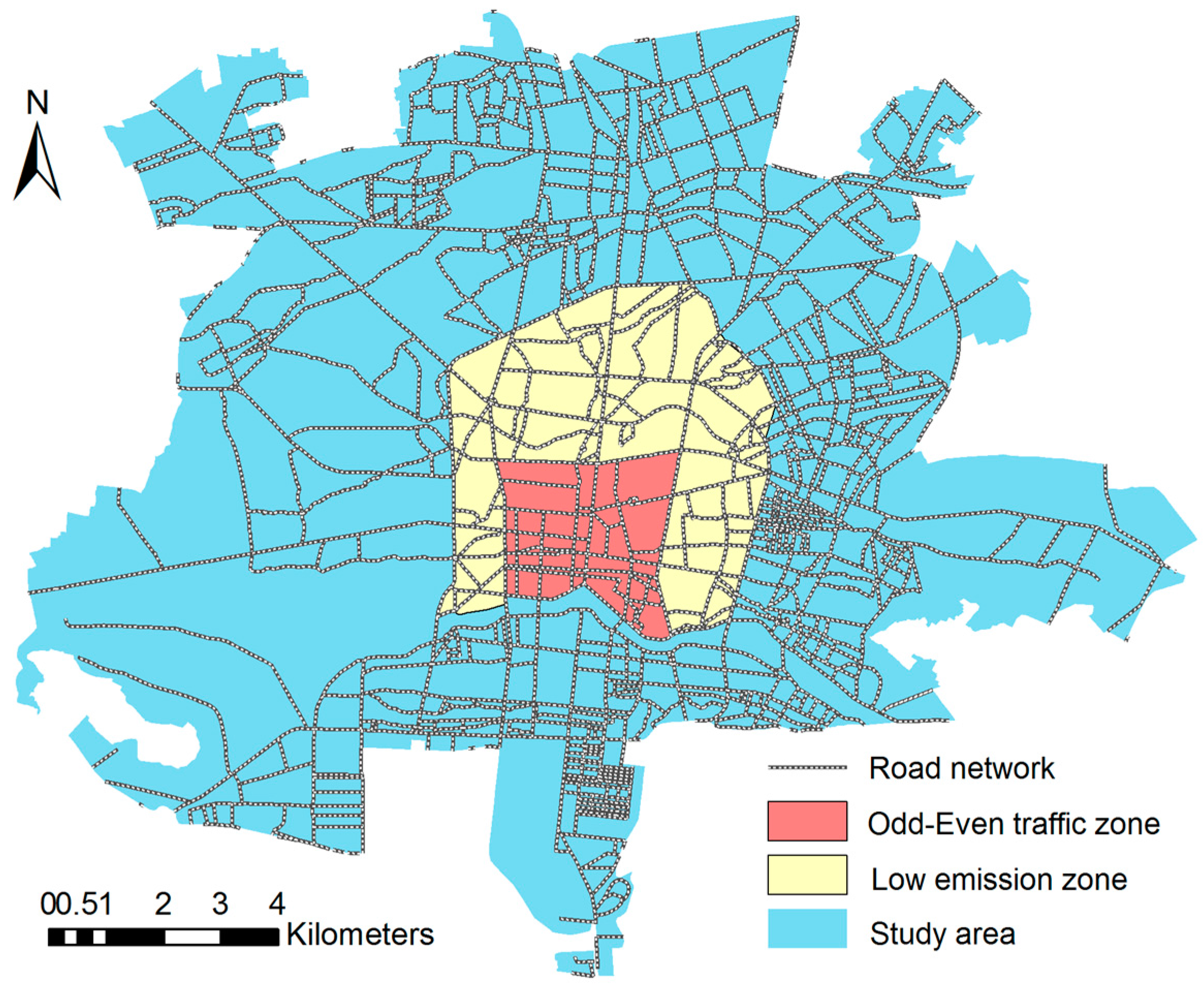
  • Odd/Even scenario is one of the most important plans proposed to cope with air pollution in Isfahan. This plan, however, is not successful in practice. Lack of supervision in Odd/Even zone, lack of police and citizen acceptability and cooperation, and the nature of the plan are the main reasons of failure [52]. Modeling by Transport and Traffic Department of Isfahan Municipality has determined what the traverse of transport fleet would be if the plan fully implemented (Figure 1).
  • Low emission zone [53] plan is widely applied in many countries to reduce air pollution. The studies run on the main parameters affecting air pollution in Isfahan, have presented three preliminary proposals with the objective of establishing LEZ: (1) restriction for old diesel vehicles; (2) restriction on motorcycle traffic in downtown; and (3) traffic ban for passenger cars and vans with respect to their emission levels in different zones (Figure 2). Modeling by the Transport and Traffic Department of Isfahan Municipality has determined the changes of traffic if LEZ scenario will be fully implemented.

3. An Approach for Environmental Health Impact Assessment of Urban Transportation Planning

The proposed approach consists of two main parts, which are responsible for modeling the suspended particle concentrations (PM2.5) caused by transportation system and estimation of health outcomes caused by the suspended particle concentrations (PM2.5), respectively. Hierarchical fuzzy inference systems are applied for modeling both parts. Regarding the problem under consideration, the mentioned parts are separately developed to calculate the accuracy and quality of model.

3.1. Hybrid Hierarchical Fuzzy Inference System (HIFS)

Fuzzy inference systems must be developed based on the necessities and special properties of the problem under consideration [54]. Considering the complexity of the relationship among air pollution and both the traffic parameters and the health, it is quite difficult to create knowledgebase based on expert’s knowledge. Moreover, due to high dimensionality in the EHIA, using traditional fuzzy inference systems leads to exponential increase of the number of rules and system errors. Two solutions are presented in this section to generate an accurate compact fuzzy inference system, conforming to the studied EHIA issue aspects.
The first solution is adopting the topology of the hierarchical fuzzy inference systems according to the problem [55]. Having transformed a fuzzy inference system to a number of more simple systems related to each other hierarchically, these systems reduce the number of rules. Through this approach, by considering the physical nature of the problem, a system will be developed with desirable aspects, which has increased the accuracy [56].
The second solution is to determine the number of partitions for each linguistic variable, membership function parameters and the rule sets through learning in a simultaneous manner. To this aim, after choosing a conforming topology to the problem, the NSGA2 algorithm is applied to define and tune the fuzzy inference system. Thus, the knowledgebase will be created automatically and the system accuracy and complexity will be optimized.
In the following, the components of the Heuristic algorithm with two minimization objectives are described, including the number of rules and the root mean square error (RMSE).
F 1 : Minimize ( i = 1 n s j = 1 v i m j )
where ns is the number of fuzzy subsystems, vi is the number of variables related to each subsystem, and mj is the number of membership functions.
F 2 : Minimize ( 1 n c 1 i = 1 n c ( F ( x i ) y i ) 2 )
where nc is the number of instances, F ( x i ) is the output from fuzzy inference system, and y i is the desired output based on the instances.
A triploid scheme is used to encode the chromosome (Equation (3)). CL is used to determine the number of membership functions related to each variable, CT is used to tune the membership functions, and CC is used for the rules consequence parts.
C = CL + CT + CC
A vector of integer numbers with size n + ns 1 is used to encode CL part (Equation (4)). n is the number of input variables and ns − 1 is the number of linking variables made to link different subsystems. Each gene ( C l ( i ) ) takes values in the set {1, …, 7}. These numbers indicate the number of fuzzy membership functions used by each variable. Variables taking a value equal to 1 do not remain in the system.
C L = { c l ( 1 ) , ... , c l ( n + n s 1 ) }
The lateral displacement [57] is applied to tune the membership functions. This method allows for the lateral displacement of each membership function partition only by using one parameter. Hence, the search area becomes smaller and more fuzzy inference systems can be analyzed to obtain a desirable answer. A vector of real numbers is used for encoding in CT part (Equation (5)). These numbers may displace in a predetermined range.
C T =   { c t ( 1 , 1 ) ,   ,   c t ( 1 , c l ( 1 ) ) ,     ,   c t ( n + n s 1 , c l ( n + n s 1 ) ) }
where the number of variables equals n + ns − 1 and each is described through C l ( i ) fuzzy membership function. A vector of real numbers is used for encoding in CC part (Equation (6)). With this encoding, the output of each rule is defined by a [0 1] number.
C C   = { c c ( 1 , 1 ) ,   ,   c c ( 1 , m 1 v 1 ) ,     ,   c c ( n s , m n s v n s ) }
The initial population is generated randomly. To generate the CL part, random values from {1, …, 7} are assigned to the related genes. Upon the generation of the CL part for each chromosome, two different versions are generated in the CT part. Random real numbers in an interval of ( ( c t ( i , j + 1 ) c t ( i , j ) ) / 2 ) are assigned in both positive and negative directions from the partition center in these versions. C t ( i , j ) indicates the center of the jth partition of the ith variable. A random number from [0 1] is assigned to each gene in the CC part of each chromosome.
The crossover and mutation operators are applied to examine different configurations and optimize the solutions. The crossover operators are selected separately for each chromosome part. The BLX method is applied for the CT and CC parts, where real numbers are used for encoding [58]. This crossover method is widely used in genetic encoding of real numbers. The standard two-point crossover method is used in the CL part. The mutation operator is applied to all produced offspring. Finally, after both operators were applied, the two more accurate offspring are considered as the new generation.

3.2. Hierarchical Fuzzy Inference Model for Modeling Traffic Related PM2.5

Using the suggested system in Section 3.1, a hierarchical fuzzy inference system is proposed here to estimate the traffic-related suspended particles concentration (PM2.5). This system is developed applying AERMOD dispersion model receptors as the dependent variable, and the transportation parameters including traffic volume, emission factor, and road network as independent variables (Figure 3).
AERMOD is the dispersion model recommended by the United States Environmental Protection Agency (EPA). This dispersion model was used in numerous EHIAs for modeling the pollution caused by a specific source of emission [59,60,61,62,63,64,65].
Utilizing the dispersion model receptors not only models the causal relationship between transportation and PM2.5 concentration, but also compensates the drawback of low spatial density of samples that are used to develop the model [30]. Due to the number and coverage of these receptors in comparison with air pollution monitoring stations, the proposed approach provide more robust model. Moreover, employing these receptors in developing the HFIS will improve the model accuracy by modeling the interactions between emission sources and meteorological processes [12,20,26]. On the other hand, the independent variables include parameters that are affected by different transportation scenarios, considering the uncertainties in modeling the causal relationship will provide the required flexibility in the proposed model to be used in impact assessments.

3.3. Hierarchical Fuzzy Inference System for Modeling Health Impacts

3.3.1. Health Impact Metrics for Air Pollution Scenario Assessment

A variety of HIA metrics have been developed to estimate the impact of PM2.5 on health [31]. The log-linear model (Equations (7) and (8)) is the most common metric in recent quantitative HIAs which endorsed by WHO. This model links PM2.5 concentration and health outcomes [9,66,67,68].
R R = e β × P M exposure
Δ y = y 0 × ( R R 1 ) R R = y 0 × ( e β × P M exposure 1 ) e β × P M exposure = y 0 × ( 1 e β × P M exposure )
where β is the concentration-response coefficient that determines the impact of PM2.5 concentration on health outcome. RR is the relative risk of that health outcome. y0 is the observed total instances of the health outcome due to all factors among the same population and in the same location. Δy is the number of cases of adverse health event attributed to PM2.5 due to the studied scenario.

3.3.2. Converting Health Impact Metric to the Hierarchical Fuzzy Inference System

Despite the importance of providing detailed information about health outcomes for planning and management, only some developed countries possess such information. Concentration-response coefficients (β) and baseline health outcome is obtained from limited studies performed in the study area or from similar studies in other regions, especially in developing countries. Fuzzy logic is the best tool for describing such parameters. Regarding the uncertainty in the parameters and the metric itself, a hierarchical fuzzy inference system was developed in this study to estimate health outcomes of traffic related PM2.5.
The topology of the proposed hierarchical system is developed based on Equations (7) and (8) (Figure 4). Evidence from previous researches, including the study by the authors, have proven that the conformity between the hierarchical structure and the studied issue considerably improve the performance [55,56].

4. Practical Evaluation

To determine the efficiency of this proposed approach, it is implemented in assessing the environmental health outcomes caused by transportation scenarios.

4.1. Data Preparation and Experimental Setup

The AERMOD code (v.15181) is applied to generate the dependent variable of hierarchical fuzzy inference system in modeling the PM2.5 concentration (HFISPM). Adopting the AERMOD dispersion model requires meteorological data, landuse, land cover, and traffic data. The data preparation is made according to the quantitative analysis guidance of traffic related PM [69].
The meteorological data include temperature, humidity, dew-point temperature, wind speed, wind direction, pressure (from the sea level), pressure (local), and cloud coverage. These data are obtained on an hourly basis from a synoptic station at Isfahan, Iran, for a five-year period. The land use and land cover data are extracted from the 1:2000 maps of the Isfahan municipality. The traffic data consist of emission factors and traffic volume. The emission factors were obtained from studies that take place about transportation fleet in Iran [70,71] (Table 2).
The traffic volume is produced through modeling the traffic demand with a four-step model and provides by the Traffic and Transportation Department of Isfahan municipality. This four-step model determines the demand on roadways. The four steps consist of trip generation, trip distribution, mode choice, and trip assignment. In the first step, the socioeconomic data are used to determine trip frequency. The trip ends, trip productions and trip attractions are determined in a separate manner. In the second step, the produced trips are distributed based on several parameters including the number of trip productions, the number of trip attractions, and travel time and/or cost. In the third step, the modes of trips are determined. Finally, the trips from mode choice are assigned to mode-specific networks [72]. These four steps represent the basic building blocks of Isfahan municipality transportation model which is implemented in Emme 4 environment. The outputs of this model consist of the traffic volume and speed of each vehicle type for main road networks. The emission level caused by each road link is computed through Equation (9).
E R i = E F i j · N i j · L i A i · T i
where ERi is the emission rate from link i, EFij is the emission factor for vehicle class j passed through the link i, Nij is the number of vehicle trips for vehicle class j passed in Ti time through link i, Li is the length of link i, and Ai is the area of link i. The road network is divided into 1 km2 grid and each cell is used as emission source in an individual model run.
In dispersion model, the 163 receptors are defined according to the district center coincidence. In this manner, the receptors located in various urban contexts coincide with the population centers; moreover, such a distribution can lead to robustness of the fuzzy model. Regarding the objective of this study, i.e., quantitative EHIA of traffic scenarios, the annual mean concentration from dispersion model is applied (Figure 5).
A buffer analysis is applied around all dispersion model receptors to generate the independent variables related to traffic volume and road network area. The radii of the buffers are 500 m. The buffer distance is selected according to evidence, indicating extension of gradients from road network [73,74,75], and LUR studies [10,16,56]. Domain of the independent variables for HFISPM model is tabulated in Table 3.
Concentration-response coefficients and baseline health outcome rates applied in modeling are tabulated in Table 4. In this article, the coefficients are obtained from meta-analysis studies instead of local studies as recommended by WHO. The level of exposure is evaluated by overlaying the concentration map and census block map. This method has been used in most prior studies to assess health outcomes as an accepted method [9,64]; because, on the one hand, the required data for modeling the exposure of total population are only available in this form, and, on the other hand, this method does not have considerable influence on exposure estimates, at the city scale [76].
A five-fold cross-validation technique is applied in all evaluations; hence, the instances are divided into five classes: four for training and one for testing the system, repeated for five times.
The algorithm parameters for all evaluations are as follows: The maximum number of iterations equal 1000, initial population equal 200, crossover rate equal 0.8, and the mutation rate equal 0.2. Since analyzing the sensitivity of these parameters is beyond the scope of this study, they are selected based on usual standards applied in heuristic studies.

4.2. Results and Discussion

4.2.1. Implementation and Evaluation of Hierarchical Fuzzy Inference Systems

The following models are developed based on this proposed approach: one for modeling the PM2.5 concentration (HFISPM) and three for estimating the health outcomes due to PM2.5, including the total mortality (HFISTM), cardiovascular mortality (HFISCM) and respiratory mortality (HFISRM).
The Pareto fronts produced by a single run of this proposed algorithm for each model is shown in Figure 6. This algorithm covers the Pareto fronts in all four models in an appropriate manner. The number of rule’s range and accuracy (RMSE) differ with respect to the studied issue in this article. As observed in Figure 6, the numbers of rule’s range are not significantly different in the three models estimating health outcomes. In general, the more the number of input parameter, the more the rules produced to describe the system.
In this study, the most accurate solution (hierarchical fuzzy inference system) from each Pareto front is applied for assessments. It is necessary to note that although the number of rules, as the index of model complexity, and RMSE as the index of model accuracy make a multi-objective problem, the simultaneous optimization of these indexes leads to a better cooperation among the produced rules, thus improving the model accuracy [56].
The average RMSE for training (RMSETra) and test (RMSETst) datasets and the average number of rules (R) for each model are tabulated in Table 5. Because the five-fold cross-validation technique is applied in all experiments here, the result for each model is considered as the average of the five runs.
Considering the 11 inputs for the HFISPM model and four inputs for the health models, and assuming five membership functions for each input are required, in conventional fuzzy inference systems, 511 = 48,828,125 and 54 = 625 rules are necessary, while this newly proposed model achieved a high accuracy with significantly fewer rules.
RMSE can be applied to compare this proposed model with conventional LUR models. The range and variation of the data must be considered for this intended purpose. Based on the reviews performed on the LUR domain [10,16], the RMSEs range for the PM2.5 is within 0.8 to 3.3, which is about 50% of the standard deviation of respective data. In this study, the measured standard deviation for PM2.5 from the dispersion model is 6 μg/m3. Therefore, the accuracy here is appropriate for measuring the PM2.5 concentration.
The PM2.5 concentration obtained from the dispersion model receptors compared with the predicted concentration in the training and test datasets are shown in Figure 7 where coefficients of determination (R2) are 0.81 and 0.75 for these two datasets, respectively. As observed in this figure, the proposed model has a significant predictive power for the whole range of PM2.5 concentration.
The histogram of the difference between PM2.5 concentrations obtained from this proposed model and the dispersion model is shown in Figure 8. Where, the distribution of this difference is near normal. This difference is random and independent from station location. Here, there exists no systematic error in estimating the concentrations. By applying more receptors placed in various urban contexts in this model, it is less sensitive to inputs and yields more certain predetermined accuracy.
The monitoring stations are used for external validation of this proposed model. There are nine air pollution monitoring stations installed in heavy traffic areas in the city of Isfahan which have applicable annual PM2.5 samples (Figure 9).
This proposed model is applied at the same locations to estimate the traffic related PM2.5 concentration. These two datasets have statistically significant correlation (r = 0.76) (Figure 10).
The only source apportionment dataset in the study area is obtained from comprehensive fugitive dust and particulate matter control plan in the central Isfahan province [78]. In this plan, positive matrix factorization (PMF), [79] is applied to apportion the sources on the basis of observations at three sampling stations. PMF is a widely used multivariate factor analysis tool, because it does not require detailed data [80] and there are various software platforms that can perform this analysis [81]. According to the PMF analysis, the primary PM emissions from vehicle exhaust constitute about 49% of the PM2.5. The contribution of traffic related PM2.5 from HFIS model is about 55% of the monitoring station concentration. The results indicate that HFIS model has an accuracy of about 12% compared with the source apportionment method.
After optimization, nine input variables remain in HFISPM model. The initial and final partitions for each input, linking, and output variables as the results of a single run of HFISPM model are shown in Figure 11. The variables related to traffic volume are described with more partitions than that of the related to emission factors. This indicates the influence of variables’ range on the number of required fuzzy partitions. The highways and arterials are described with more fuzzy partitions than the residential roads. Regarding the similar range of these variables, different number of partitions indicates the higher influence of highways and arterials on PM2 production.
The control surface plots for census block versus baseline health outcome rate, PM2.5 concentration versus concentration response coefficient, and total adverse health outcome versus relative risk are shown in Figure 12. These plots are derived from the generated rules of the respective FISs, which they depict the dependency of the outputs as a function of the inputs. Moreover, these plots indicate the consistency of the rules in HFISTM model.

4.2.2. Scenarios Evaluations

A grid of HFISPM model receptors located 100 meters apart is used in assessing the scenarios. With this spatial resolution, small-scale variation of the pollution will be modeled as well. The PM2.5 concentration map for the first scenario (the current condition) is shown in Figure 13a. As expected, the PM2.5 concentration is higher along the roads and at interchanges. However, there is exist PM2.5 concentration all over the study area. In the first scenario, the mean, minimum, and maximum of traffic related PM2.5 concentrations are 19 μg/m3, 11 μg/m3, and 58 μg/m3, respectively. Although the traffic is responsible for 70% of PM2.5 emission over the city, the annual mean of PM2.5 concentration measured by the air pollution monitoring stations is about 70 μg/m3. This difference is caused by both the dust haze phenomenon in the study region and the background pollution.
In the second scenario, the mean, minimum, and maximum of traffic related PM2.5 concentrations are 20 μg/m3, 11 μg/m3, and 59 μg/m3, respectively (Figure 13b). In this scenario, the concentration is increased about 7% in the Odd/Even zone with a mean of about 1%. This scenario leads to a decrease in traffic volume during the traffic restrictions hours in the aforementioned zone; while due to constant travel demands, the traffic of other vehicles including buses, motorcycles and taxies has increased in this area. On the other hand, the traffic volume out of the restriction hours is increased.
In the third scenario, the mean, minimum, and maximum of traffic related PM2.5 concentrations are 12 μg/m3, 6 μg/m3, and 36 μg/m3, respectively (Figure 13c). In this scenario, a considerable decrease in PM2.5 concentration is observed. The main reason here is the low emission standard of the current fleet in the study area and the prohibition of their traffic based on the low emission zone scenario.
Using this proposed HFIS model for modeling the PM2.5 concentration has many advantages in comparison with the dispersion model or the conventional LURs. Estimating concentration over the study area in applied resolution with dispersion model, by considering 18,759 receptors, 756 roads, 8760 h per year, and a five-year period necessitated for impact assessment (IA), requires 621 billion source-receptor computations. These intensive computations require many years to be completed with a standard workstation. Moreover, using dispersion model needs intensive inputs, like meteorological data, which do not exist. especially for the future scenarios. These problems lead to lesser use of the dispersion models in the health impact assessment studies compared to the LUR models [23]. On the contrary, the conventional LUR models are encountering problems in modeling the PM2.5 concentration with high resolutions due to not considering the interaction between emissions and meteorological processes. In addition to solving the problem of intensive data and processing caused by dispersion models, this proposed model possesses the benefits of LUR models including flexibility in the required inputs. Through making application of uncertain data possible, this approach provides the requirements of the environmental health impact assessments, and can be integrated into the planning and decision-making processes. It should be mentioned that one of the limitations of this study is the propagation of the intrinsic error of the dispersion model in the HFIS model. This limitation is common in nearly all studies which integrate the dispersion and regression models to overcome their drawbacks [26,28,29,30,65]. However, these studies reveal that, despite this limitation, especially when a specific source of pollution is to be modeled, applying the dispersion models in generating the regression model contributes to model accuracy improvement.
The mortality due to each scenario is shown in Table 6. As indicated, the best and worse scenarios are the third and the second, respectively, regarding their outcomes on health.
This proposed model is an appropriate alternative for Equations (7) and (8) applied in most studies to estimate health outcomes, whereas the relationship among their parameters, like the concentration-response coefficient β, baseline health outcome, and adverse attributable health outcome is not exactly known. The ability of learning and tuning in this proposed model provides the opportunity to model the uncertainty in the relationship among model parameters. This proposed model is an interpretable model developed based on existing epidemiologic evidences, and it can consider the parameter uncertainties; therefore, it has several advantages in comparison with conventional deterministic metrics [31].

5. Conclusions

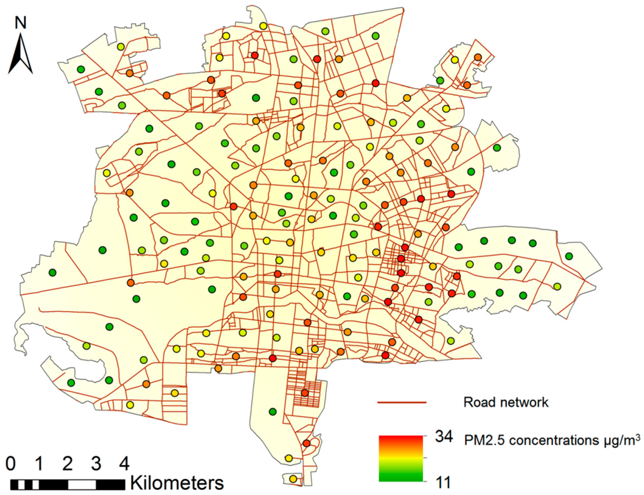
A new quantitative modeling approach for environmental health impact assessment of transportation scenarios was proposed in this study, where optimized hierarchical fuzzy inference systems was employed for modeling the impacts of traffic on PM2.5 concentrations and the effects of traffic related PM2.5 on health.
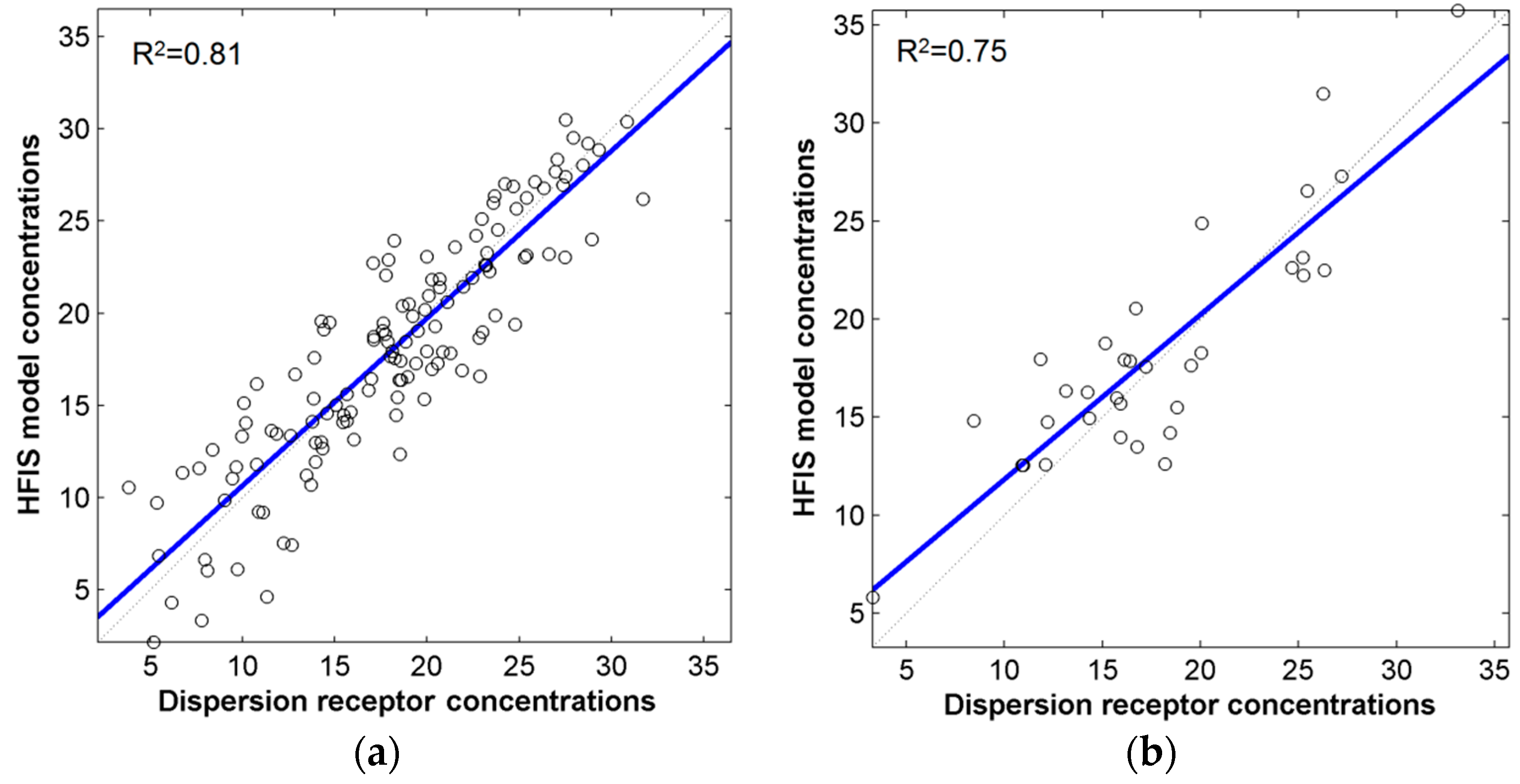
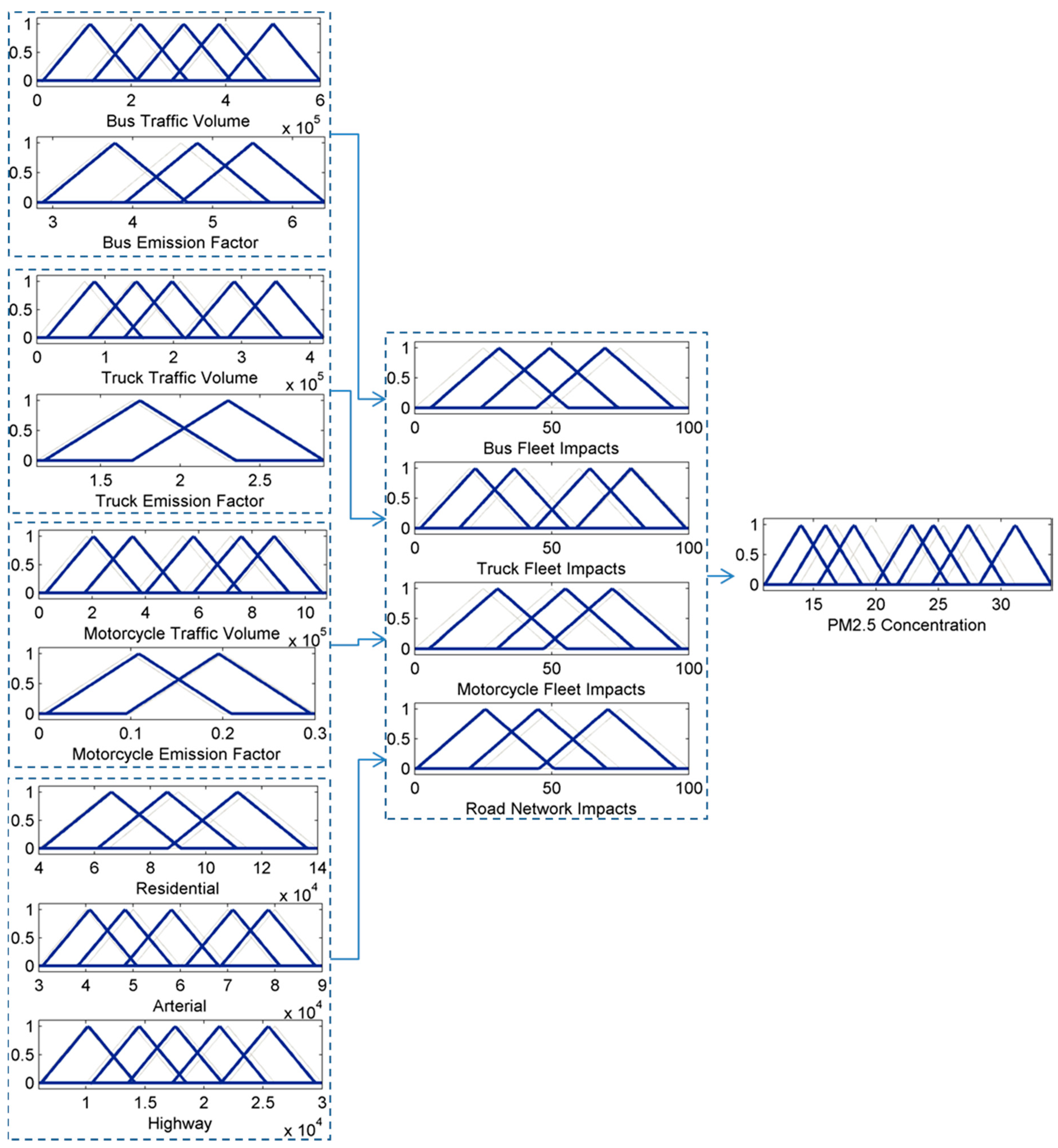
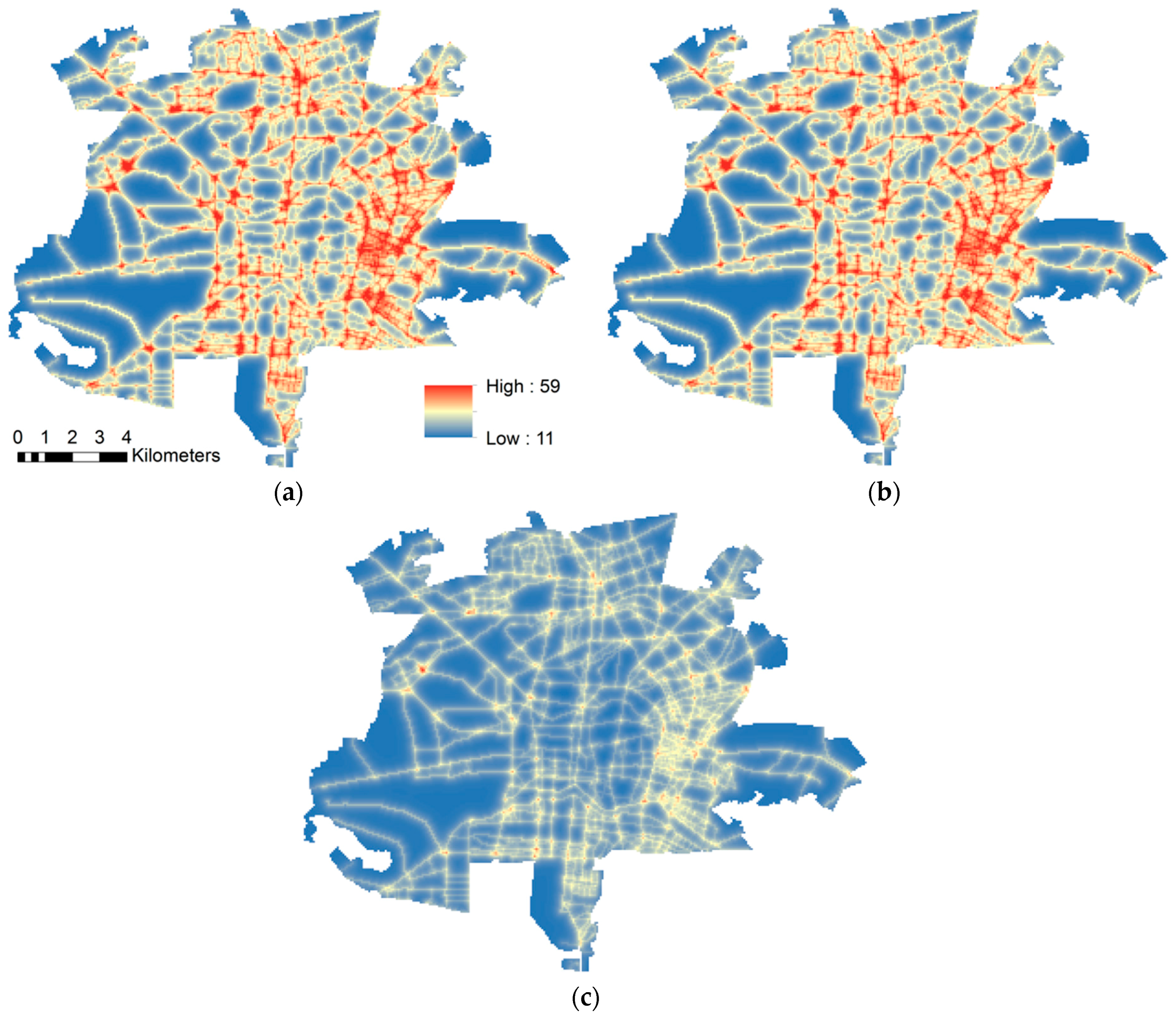
AERMOD dispersion receptors were used as dependent variables, and transportation parameters were used as independent variables to develop the hierarchical fuzzy inference system for modeling PM2.5 concentration (HFISPM). Integration of HFIS and dispersion model is one of the main contributions of this article. Compared to conventional models, the HFIS has several advantages, like appropriate processing requirements, selectable inputs, consideration of interaction between emissions and meteorological processes, and modeling the casual relationship among transportation parameters and air pollution. Due to the capability of applying qualitative and quantitative data, this proposed model could be adopted in environmental health impact assessment. High spatial resolution of derived PM2.5 map can provide essential information to assess the impacts of various scenarios on health.
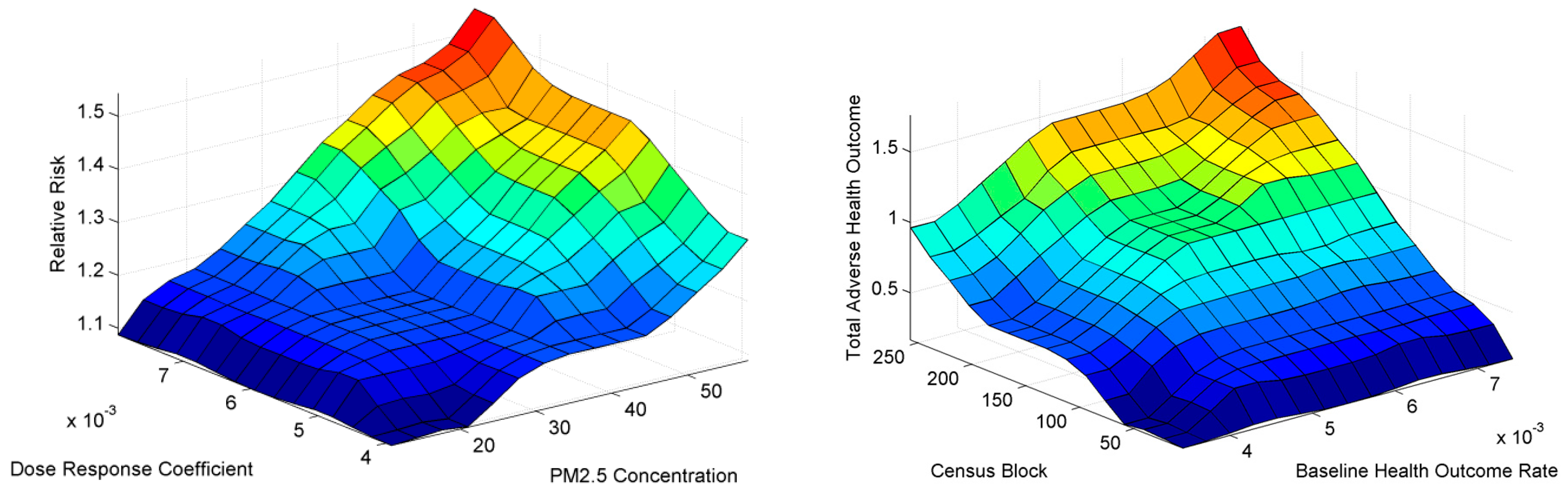
This proposed hierarchical fuzzy inference system for modeling health outcome was developed based on the epidemiological equations. Although these relations are frequently applied in health impact assessment, they are subject of debate in many related studies. The capability of learning and tuning of relationships in this proposed approach enables the modeling of the uncertainty of relationships among parameters and the uncertainty associated with parameter values in a simultaneous manner.
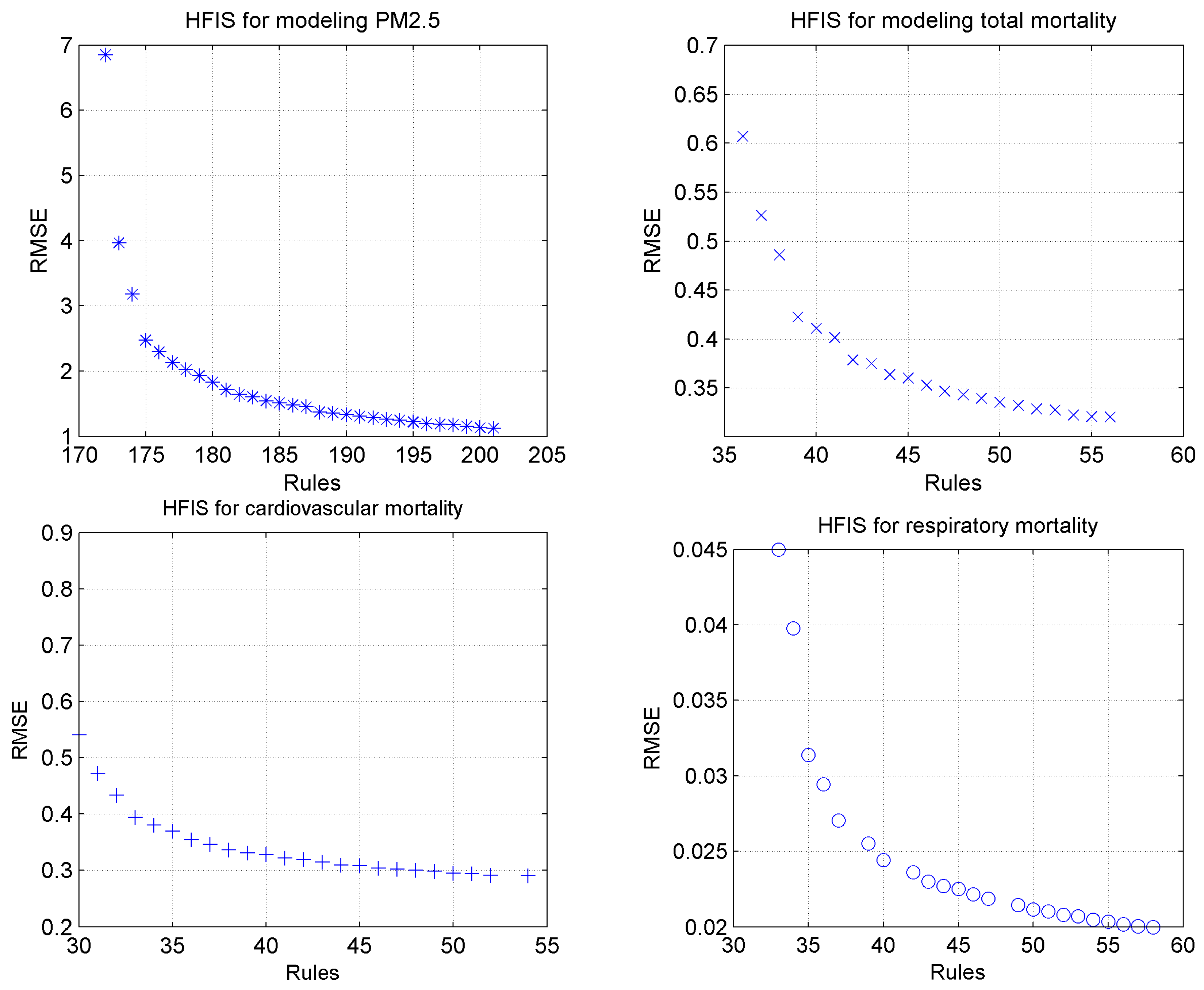
In order to design the fuzzy inference systems according to the problem requirements, to be able to overcome the exponential increase of rules, and to increase accuracy, two solutions were applied. The first solution is to select the topology of the hierarchical fuzzy inference system according to the problem. The second solution is the concurrent determination of the membership functions and rule set through learning. These two solutions have led to a better cooperation between the generated rules in knowledge base of models, maximization of accuracy, and minimization of system complexity.
Three traffic scenarios, the current condition, Odd/Even, and LEZ, were assessed here. The modeling results indicate that LEZ has the most advantages associated with air pollution and health. Applying hierarchical fuzzy inference system in EHIA can provide better understanding of the issue for planners and decision makers. Moreover, decision makers can assess the impact of changes in each parameter better.

Acknowledgments

The authors acknowledge the Isfahan Municipality, Meteorological, and Environmental Protection Organizations to have provided whole basic datasets and report documents. Especially, we would like to thanks the experts of Transport and Traffic Department of Isfahan Municipality for their constructive suggestions and remarks that greatly helped us to improve the contents of this paper.

Author Contributions

Behnam Tashayo conceived and designed the experiments, carried out model development and verification the models, and drafted the original version of the manuscript. Abbas Alimohammadi led the study, including experimental setup, model simulations and evaluation, and revisions of the paper. Mohammad Sharif assisted with analysis of the scenarios, edited, and helped to revise the paper. All authors read and approved the final manuscript.

Conflicts of Interest

The authors declare no conflict of interest.

References

  1. Hebert, K.A.; Wendel, A.M.; Kennedy, S.K.; Dannenberg, A.L. Health impact assessment: A comparison of 45 local, national, and international guidelines. Environ. Impact Assess. Rev. 2012, 34, 74–82. [Google Scholar] [CrossRef]
  2. Mesa-Frias, M.; Chalabi, Z.; Vanni, T.; Foss, A.M. Uncertainty in environmental health impact assessment: Quantitative methods and perspectives. Int. J. Environ. Health Res. 2013, 23, 16–30. [Google Scholar] [CrossRef] [PubMed]
  3. Dannenberg, A.L.; Bhatia, R.; Cole, B.L.; Heaton, S.K.; Feldman, J.D.; Rutt, C.D. Use of health impact assessment in the US: 27 case studies, 1999–2007. Am. J. Prev. Med. 2008, 34, 241–256. [Google Scholar] [CrossRef] [PubMed]
  4. Singleton-Baldrey, L. The Impacts of Health Impact Assessment: A Review of 54 Health Impact Assessments, 2007–2012; University of North Carolina: Chapel Hill, NC, USA, 2012. [Google Scholar]
  5. Rhodus, J.; Fulk, F.; Autrey, B.; O’Shea, S.; Roth, A. A Review of Health Impact Assessments in the US: Current State-of-Science, Best Practices, and Areas for Improvement; Environmental Protection Agency: Cincinnati, OH, USA, 2013.
  6. White, L.; Noble, B.F. Strategic environmental assessment for sustainability: A review of a decade of academic research. Environ. Impact Assess. Rev. 2013, 42, 60–66. [Google Scholar] [CrossRef]
  7. Kentel, E.; Aral, M. 2D monte carlo versus 2D fuzzy monte carlo health risk assessment. Stoch. Environ. Res. Risk Assess. 2005, 19, 86–96. [Google Scholar] [CrossRef]
  8. Arunraj, N.; Mandal, S.; Maiti, J. Modeling uncertainty in risk assessment: An integrated approach with fuzzy set theory and monte carlo simulation. Accid. Anal. Prev. 2013, 55, 242–255. [Google Scholar] [CrossRef] [PubMed]
  9. Chart-asa, C.; Gibson, J.M. Health impact assessment of traffic-related air pollution at the urban project scale: Influence of variability and uncertainty. Sci. Total Environ. 2015, 506, 409–421. [Google Scholar] [CrossRef] [PubMed]
  10. De Hoogh, K.; Korek, M.; Vienneau, D.; Keuken, M.; Kukkonen, J.; Nieuwenhuijsen, M.J.; Badaloni, C.; Beelen, R.; Bolignano, A.; Cesaroni, G. Comparing land use regression and dispersion modelling to assess residential exposure to ambient air pollution for epidemiological studies. Environ. Int. 2014, 73, 382–392. [Google Scholar] [CrossRef] [PubMed]
  11. Dockery, D.W.; Pope, C.A.; Xu, X.; Spengler, J.D.; Ware, J.H.; Fay, M.E.; Ferris, B.G., Jr.; Speizer, F.E. An association between air pollution and mortality in six us cities. N. Engl. J. Med. 1993, 329, 1753–1759. [Google Scholar] [CrossRef] [PubMed]
  12. Jerrett, M.; Arain, A.; Kanaroglou, P.; Beckerman, B.; Potoglou, D.; Sahsuvaroglu, T.; Morrison, J.; Giovis, C. A review and evaluation of intraurban air pollution exposure models. J. Expo. Sci. Environ. Epidemiol. 2005, 15, 185–204. [Google Scholar] [CrossRef] [PubMed]
  13. Miller, K.A.; Siscovick, D.S.; Sheppard, L.; Shepherd, K.; Sullivan, J.H.; Anderson, G.L.; Kaufman, J.D. Long-term exposure to air pollution and incidence of cardiovascular events in women. N. Engl. J. Med. 2007, 356, 447–458. [Google Scholar] [CrossRef] [PubMed]
  14. Kheirbek, I.; Wheeler, K.; Walters, S.; Kass, D.; Matte, T. PM2.5 and ozone health impacts and disparities in New York city: Sensitivity to spatial and temporal resolution. Air Qual. Atmos. Health 2013, 6, 473–486. [Google Scholar] [CrossRef] [PubMed]
  15. Batterman, S.; Chambliss, S.; Isakov, V. Spatial resolution requirements for traffic-related air pollutant exposure evaluations. Atmos. Environ. 2014, 94, 518–528. [Google Scholar] [CrossRef] [PubMed]
  16. Hoek, G.; Beelen, R.; de Hoogh, K.; Vienneau, D.; Gulliver, J.; Fischer, P.; Briggs, D. A review of land-use regression models to assess spatial variation of outdoor air pollution. Atmos. Environ. 2008, 42, 7561–7578. [Google Scholar] [CrossRef]
  17. Clougherty, J.E.; Kheirbek, I.; Eisl, H.M.; Ross, Z.; Pezeshki, G.; Gorczynski, J.E.; Johnson, S.; Markowitz, S.; Kass, D.; Matte, T. Intra-urban spatial variability in wintertime street-level concentrations of multiple combustion-related air pollutants: The New York city community air survey (NYCCAS). J. Expo. Sci. Environ. Epidemiol. 2013, 23, 232–240. [Google Scholar] [CrossRef] [PubMed]
  18. Basagaña, X.; Aguilera, I.; Rivera, M.; Agis, D.; Foraster, M.; Marrugat, J.; Elosua, R.; Künzli, N. Measurement error in epidemiologic studies of air pollution based on land-use regression models. Am. J. Epidemiol. 2013, 178, 1342–1346. [Google Scholar] [CrossRef] [PubMed]
  19. Alexeeff, S.E.; Schwartz, J.; Kloog, I.; Chudnovsky, A.; Koutrakis, P.; Coull, B.A. Consequences of kriging and land use regression for PM2.5 predictions in epidemiologic analyses: Insights into spatial variability using high-resolution satellite data. J. Expo. Sci. Environ. Epidemiol. 2015, 25, 138–144. [Google Scholar] [CrossRef] [PubMed]
  20. Su, J.G.; Brauer, M.; Ainslie, B.; Steyn, D.; Larson, T.; Buzzelli, M. An innovative land use regression model incorporating meteorology for exposure analysis. Sci. Total Environ. 2008, 390, 520–529. [Google Scholar] [CrossRef] [PubMed]
  21. Wilton, D.C. Modelling Nitrogen Oxides in Los Angeles Using a Hybrid Dispersion/Land Use Regression Model; University of Washington: Seattle, WA, USA, 2011. [Google Scholar]
  22. HEI. Traffic-Related Air Pollution: A Critical Review of the Literature on Emissions, Exposure, and Health Effectsspecial Reports; HEI: Honolulu, HI, USA, 2010. [Google Scholar]
  23. Brauer, M.; Ainslie, B.; Buzzelli, M.; Henderson, S.; Larson, T.; Marshall, J.; Nethery, E.; Steyn, D.; Su, J. Models of exposure for use in epidemiological studies of air pollution health impacts. In Air Pollution Modeling and Its Application XIX; Springer: Berlin, Germany, 2008; pp. 589–604. [Google Scholar]
  24. Michanowicz, A. Hybrid Dispersion/Land Use Regression Modeling for Improving Air Pollutant Concentration Estimates; University of Pittsburgh: Pittsburgh, PA, USA, 2015. [Google Scholar]
  25. Marshall, J.D.; Nethery, E.; Brauer, M. Within-urban variability in ambient air pollution: Comparison of estimation methods. Atmos. Environ. 2008, 42, 1359–1369. [Google Scholar] [CrossRef]
  26. Wilton, D.; Szpiro, A.; Gould, T.; Larson, T. Improving spatial concentration estimates for nitrogen oxides using a hybrid meteorological dispersion/land use regression model in Los Angeles, CA and Seattle, WA. Sci. Total Environ. 2010, 408, 1120–1130. [Google Scholar] [CrossRef] [PubMed]
  27. Lindström, J.; Szpiro, A.A.; Sampson, P.D.; Oron, A.P.; Richards, M.; Larson, T.V.; Sheppard, L. A flexible spatio-temporal model for air pollution with spatial and spatio-temporal covariates. Environ. Ecol. Stat. 2014, 21, 411–433. [Google Scholar] [CrossRef] [PubMed]
  28. Isakov, V.; Touma, J.S.; Burke, J.; Lobdell, D.T.; Palma, T.; Rosenbaum, A.; kÖzkaynak, H. Combining regional-and local-scale air quality models with exposure models for use in environmental health studies. J. Air Waste Manag. Assoc. 2009, 59, 461–472. [Google Scholar] [PubMed]
  29. Johnson, M.; Isakov, V.; Touma, J.; Mukerjee, S.; Özkaynak, H. Evaluation of land-use regression models used to predict air quality concentrations in an urban area. Atmos. Environ. 2010, 44, 3660–3668. [Google Scholar] [CrossRef]
  30. Mölter, A.; Lindley, S.; de Vocht, F.; Simpson, A.; Agius, R. Modelling air pollution for epidemiologic research—Part i: A novel approach combining land use regression and air dispersion. Sci. Total Environ. 2010, 408, 5862–5869. [Google Scholar] [CrossRef] [PubMed]
  31. Martenies, S.E.; Wilkins, D.; Batterman, S.A. Health impact metrics for air pollution management strategies. Environ. Int. 2015, 85, 84–95. [Google Scholar] [CrossRef] [PubMed]
  32. Walker, W.E.; Harremoës, P.; Rotmans, J.; van der Sluijs, J.P.; van Asselt, M.B.; Janssen, P.; von Krauss, M.P.K. Defining uncertainty: A conceptual basis for uncertainty management in model-based decision support. Integr. Assess. 2003, 4, 5–17. [Google Scholar] [CrossRef]
  33. Briggs, D.J.; Sabel, C.E.; Lee, K. Uncertainty in epidemiology and health risk and impact assessment. Environ. Geochem. Health 2008, 31, 189–203. [Google Scholar] [CrossRef] [PubMed] [Green Version]
  34. Ryan, L. Epidemiologically based environmental risk assessment. Stat. Sci. 2003, 18, 466–480. [Google Scholar] [CrossRef]
  35. Leung, W.; Noble, B.; Gunn, J.; Jaeger, J.A. A review of uncertainty research in impact assessment. Environ. Impact Assess. Rev. 2015, 50, 116–123. [Google Scholar] [CrossRef]
  36. Ryan, L. Combining data from multiple sources, with applications to environmental risk assessment. Stat. Med. 2008, 27, 698–710. [Google Scholar] [CrossRef] [PubMed]
  37. Hobbs, B.F.; Stakhiv, E.Z.; Grayman, W.M. Impact evaluation procedures: Theory, practice, and needs. J. Water Resour. Plan. Manag. 1989, 115, 2–21. [Google Scholar] [CrossRef]
  38. Veerman, J.; Barendregt, J.; Mackenbach, J. Quantitative health impact assessment: Current practice and future directions. J. Epidemiol. Community Health 2005, 59, 361–370. [Google Scholar] [CrossRef] [PubMed]
  39. Stoeglehner, G. Enhancing sea effectiveness: Lessons learnt from austrian experiences in spatial planning. Impact Assess. Proj. Apprais. 2010, 28, 217–231. [Google Scholar] [CrossRef]
  40. Hosseiniebalam, F.; Ghaffarpasand, O. The effects of emission sources and meteorological factors on sulphur dioxide concentration of great isfahan, Iran. Atmos. Environ. 2015, 100, 94–101. [Google Scholar] [CrossRef]
  41. Karimi, H.; Soffianian, A.; Mirghaffari, N.; Soltani, S. Determining air pollution potential using geographic information systems and multi-criteria evaluation: A case study in isfahan province in Iran. Environ. Process. 2016, 3, 229–246. [Google Scholar] [CrossRef]
  42. Zarrabi, A.; Mohammadi, J.; Abdollahi, A. Evaluation of mobile and stationary sources of Isfahan air pollution (in persian). Geography 2010, 26, 151–164. [Google Scholar]
  43. Han, X.; Naeher, L.P. A review of traffic-related air pollution exposure assessment studies in the developing world. Environ. Int. 2006, 32, 106–120. [Google Scholar] [CrossRef] [PubMed]
  44. Karagulian, F.; Belis, C.A.; Dora, C.F.C.; Prüss-Ustün, A.M.; Bonjour, S.; Adair-Rohani, H.; Amann, M. Contributions to cities’ ambient particulate matter (PM): A systematic review of local source contributions at global level. Atmos. Environ. 2015, 120, 475–483. [Google Scholar] [CrossRef]
  45. Arfaeinia, H.; Kermani, M.; Aghaei, M.; Bahrami Asl, F.; Karimzadeh, S. Comparative investigation of health quality of air in Tehran, Isfahan and Shiraz metropolises in 2011–2012. J. Health Field 2014, 1, 37–44. [Google Scholar]
  46. Mansouri, B.; Hamidian, A.H. Assessment of the air quality of isfahan city, Iran, using selected air quality parameters. J. Int. Environ. Appl. Sci. 2013, 8, 10. [Google Scholar]
  47. DOE. Isfahan Department of Environment. Available online: http://isfahan-doe.ir/ (accessed on 28 December 2016).
  48. Rusu-Zagar, G.; Rusu-Zagar, C.; Iorga, I.; Iorga, A. Air pollution particles PM10, PM2.5 and the tropospheric ozone effects on human health. Procedia-Soc. Behav. Sci. 2013, 92, 826–831. [Google Scholar] [CrossRef]
  49. Ezzati, M.; Lopez, A.D.; Rodgers, A.; Vander Hoorn, S.; Murray, C.J. Selected major risk factors and global and regional burden of disease. Lancet 2002, 360, 1347–1360. [Google Scholar] [CrossRef]
  50. WHO (World Health Organization). The World Health Report 2002: Reducing Risks, Promoting Healthy Life; World Health Organization: Geneva, Switzerland, 2002. [Google Scholar]
  51. Bart, O. Outdoor air pollution: Assessing the environmental burden of disease at national and local levels. In Environmental Burden of Disease Series; OMS: Geneva, Switzerland, 2004; Volume 5. [Google Scholar]
  52. Latifi Sara, R.M.; Solmaz, A.; Vahid, H. The Plan of First Low Emission Zone for Tehran, Iran. Available online: http://air.tehran.ir/portals/0/ReportFiles/AirPollution/New/13.pdf (accessed on 16 January 2017). (In Persian)
  53. Del Campo, A.G. Incorporating spatial data and gis to improve sea of land use plans: Opportunities and limitations: Case studies in the republic of Ireland. Doctoral 2008. [Google Scholar] [CrossRef]
  54. Ocampo-Duque, W.; Osorio, C.; Piamba, C.; Schuhmacher, M.; Domingo, J.L. Water quality analysis in rivers with non-parametric probability distributions and fuzzy inference systems: Application to the Cauca River, Colombia. Environ. Int. 2013, 52, 17–28. [Google Scholar] [CrossRef] [PubMed]
  55. Zajaczkowski, J.; Verma, B. Selection and impact of different topologies in multi-layered hierarchical fuzzy systems. Appl. Intell. 2012, 36, 564–584. [Google Scholar] [CrossRef]
  56. Tashayo, B.; Alimohammadi, A. Modeling urban air pollution with optimized hierarchical fuzzy inference system. Environ. Sci. Pollut. Res. 2016, 23, 19417–19431. [Google Scholar] [CrossRef] [PubMed]
  57. Alcalá, R.; Alcalá-Fdez, J.; Herrera, F. A proposal for the genetic lateral tuning of linguistic fuzzy systems and its interaction with rule selection. IEEE Trans. Fuzzy Syst. 2007, 15, 616–635. [Google Scholar] [CrossRef]
  58. Herrera, F.; Lozano, M.; Verdegay, J.L. Tackling real-coded genetic algorithms: Operators and tools for behavioural analysis. Artif. Intell. Rev. 1998, 12, 265–319. [Google Scholar] [CrossRef]
  59. Isakov, V.; Arunachalam, S.; Batterman, S.; Bereznicki, S.; Burke, J.; Dionisio, K.; Garcia, V.; Heist, D.; Perry, S.; Snyder, M. Air quality modeling in support of the near-road exposures and effects of urban air pollutants study (nexus). Int. J. Environ. Res. Public Health 2014, 11, 8777–8793. [Google Scholar] [CrossRef] [PubMed]
  60. Aggarwal, P.; Jain, S. Impact of air pollutants from surface transport sources on human health: A modeling and epidemiological approach. Environ. Int. 2015, 83, 146–157. [Google Scholar] [CrossRef] [PubMed]
  61. Aliyu, A.S.; Ramli, A.T.; Saleh, M.A. Assessment of potential human health and environmental impacts of a nuclear power plant (npp) based on atmospheric dispersion modeling. Atmósfera 2015, 28, 13–26. [Google Scholar] [CrossRef]
  62. Batterman, S.; Ganguly, R.; Harbin, P. High resolution spatial and temporal mapping of traffic-related air pollutants. Int. J. Environ. Res. Public Health 2015, 12, 3646–3666. [Google Scholar] [CrossRef] [PubMed]
  63. Penn, S.L.; Arunachalam, S.; Tripodis, Y.; Heiger-Bernays, W.; Levy, J.I. A comparison between monitoring and dispersion modeling approaches to assess the impact of aviation on concentrations of black carbon and nitrogen oxides at Los Angeles international airport. Sci. Total Environ. 2015, 527, 47–55. [Google Scholar] [CrossRef] [PubMed]
  64. Rowangould, G.M. A new approach for evaluating regional exposure to particulate matter emissions from motor vehicles. Transp. Res. Part D Transp. Environ. 2015, 34, 307–317. [Google Scholar] [CrossRef]
  65. Michanowicz, D.R.; Shmool, J.L.; Tunno, B.J.; Tripathy, S.; Gillooly, S.; Kinnee, E.; Clougherty, J.E. A hybrid land use regression/aermod model for predicting intra-urban variation in PM2.5. Atmos. Environ. 2016, 131, 307–315. [Google Scholar] [CrossRef]
  66. Ostro, B.; Chestnut, L. Assessing the health benefits of reducing particulate matter air pollution in the United States. Environ. Res. 1998, 76, 94–106. [Google Scholar] [CrossRef] [PubMed]
  67. Li, Y.; Gibson, J.M.; Jat, P.; Puggioni, G.; Hasan, M.; West, J.J.; Vizuete, W.; Sexton, K.; Serre, M. Burden of disease attributed to anthropogenic air pollution in the United Arab Emirates: Estimates based on observed air quality data. Sci. Total Environ. 2010, 408, 5784–5793. [Google Scholar] [CrossRef] [PubMed]
  68. Mesa-Frias, M.; Chalabi, Z.; Foss, A.M. Quantifying uncertainty in health impact assessment: A case-study example on indoor housing ventilation. Environ. Int. 2014, 62, 95–103. [Google Scholar] [CrossRef] [PubMed]
  69. United States Environmental Protection Agency. Transportation Conformity Guidance for Quantitative Hot-Spot Analyses in PM2.5 and PM10 Nonattainment and Maintenance Areas (No. Epa-420-b-10–040); United States Environmental Protection Agency: Research Triangle Park, NC, USA, 2010.
  70. JICA (Japan International Cooperation Agency). The Study on an Integrated Master Plan for Air Pollution Control in the Greater Tehran Area in the Islamic Republic of Iran; Japan International Cooperation Agency: Tokyo, Japan, 1997.
  71. Shahbazi, H.; Babaei, M.; Afshin, H.; Hosseini, V. Emission Inventory of Tehran for 1392—Mobile Sources. Available online: http://air.tehran.ir/portals/0/ReportFiles/AirPollution/New/27.pdf (accessed on 16 January 2017). (In Persian)
  72. McNally, M.G. The four step model. Handb. Transp. Model. 2007, 1, 35–41. [Google Scholar]
  73. Zhou, Y.; Levy, J.I. Factors influencing the spatial extent of mobile source air pollution impacts: A meta-analysis. BMC Public Health 2007, 7, 89. [Google Scholar] [CrossRef] [PubMed] [Green Version]
  74. Karner, A.A.; Eisinger, D.S.; Niemeier, D.A. Near-roadway air quality: Synthesizing the findings from real-world data. Environ. Sci. Technol. 2010, 44, 5334–5344. [Google Scholar] [CrossRef] [PubMed]
  75. Yazdi, M.N.; Delavarrafiee, M.; Arhami, M. Evaluating near highway air pollutant levels and estimating emission factors: Case study of Tehran, Iran. Sci. Total Environ. 2015, 538, 375–384. [Google Scholar] [CrossRef] [PubMed]
  76. Tenailleau, Q.M.; Mauny, F.; Joly, D.; François, S.; Bernard, N. Air pollution in moderately polluted urban areas: How does the definition of “neighborhood” impact exposure assessment? Environ. Pollut. 2015, 206, 437–448. [Google Scholar] [CrossRef] [PubMed]
  77. Hoek, G.; Krishnan, R.M.; Beelen, R.; Peters, A.; Ostro, B.; Brunekreef, B.; Kaufman, J.D. Long-term air pollution exposure and cardio-respiratory mortality: A review. Environ. Health 2013, 12, 1. [Google Scholar] [CrossRef] [PubMed]
  78. DOE (Isfahan Department of Environment). Comprehensive Fugitive Dust and Particulate Matter Control Plan in the Central Isfahan Province; Isfahan Department of Environment: Isfahan, Iran, 2015.
  79. Paatero, P.; Tapper, U. Positive matrix factorization: A non-negative factor model with optimal utilization of error estimates of data values. Environmetrics 1994, 5, 111–126. [Google Scholar] [CrossRef]
  80. Viana, M.; Kuhlbusch, T.; Querol, X.; Alastuey, A.; Harrison, R.; Hopke, P.; Winiwarter, W.; Vallius, M.; Szidat, S.; Prevot, A. Source apportionment of particulate matter in Europe: A review of methods and results. J. Aerosol Sci. 2008, 39, 827–849. [Google Scholar] [CrossRef]
  81. Norris, G.; Duvall, R.; Brown, S.; Bai, S. Epa Positive Matrix Factorization (PMF) 5.0 Fundamentals and User Guide; US Environmental Protection Agency Office of Research and Development: Washington, DC, USA, 2014.
Figure 1. The amount of vehicle traverse: (a) through urban road network; and (b) in Odd/Even zone.
Sustainability 09 00134 g001
Figure 2. The road network and traffic zones maps of the city of Isfahan.
Sustainability 09 00134 g002
Figure 3. Hierarchical fuzzy inference system for modeling the suspended particles caused by transportation system.
Sustainability 09 00134 g003
Figure 4. Hierarchal fuzzy inference system for modeling the health outcome caused by suspended particles.
Sustainability 09 00134 g004
Figure 5. Distribution of dispersion model receptors and suspended particles concentration caused by transportation system.
Sustainability 09 00134 g005
Figure 6. Pareto fronts resulted from multi-objective optimization algorithm for the four models.
Sustainability 09 00134 g006
Figure 7. PM2.5 concentration diagram resulted from dispersion model versus hierarchical fuzzy inference system: (a) for training datasets; and (b) for validation datasets.
Sustainability 09 00134 g007
Figure 8. Difference between dispersion model receptors and model output (μg/m3).
Sustainability 09 00134 g008
Figure 9. Distribution of air pollution monitoring stations and sampling stations.
Sustainability 09 00134 g009
Figure 10. PM2.5 concentrations from HFIS vs. monitoring stations.
Sustainability 09 00134 g010
Figure 11. Initial and tuned database for of HFISPM model.
Sustainability 09 00134 g011
Figure 12. Control surfaces of HFISTM.
Sustainability 09 00134 g012aSustainability 09 00134 g012b
Figure 13. PM2.5 concentration resulted from the HFISPM for: (a) first scenario; (b) second scenario; and (c) third scenario.
Sustainability 09 00134 g013
Table 1. Classification of vehicles based on emission standard.
Vehicle TypesEmission StandardPercentage
Personal carNone7%
Euro 113%
Euro 255%
Euro 32%
Euro 423%
BusEuro 145%
Euro 229%
Euro 325%
TruckEuro 139%
Euro 241%
Euro 320%
MotorcycleNone15%
Euro 285%
Table 2. Emission factor for vehicles fleet [71].
Emission Factor (gr/km)Road Type
ResidentialArterialHighway
Passenger car0.10.10.1
Bus6.44.92.8
Truck2.921.1
Motorcycle0.30.250.2
Table 3. Domain of independent variables of model HFISPM.
Predictor VariablesUniverse of Discourse
Passenger car traffic volume[2 × 10²–60 × 105]
Passenger car emission factor[0–0.1]
Bus traffic volume[0–6 × 10⁵]
Bus emission factor[2.8–6.4]
Truck traffic volume[0–4.2 × 10⁵]
Truck emission factor[1.1–2.9]
Motorcycle traffic volume[0–10.8 × 10⁵]
Motorcycle emission factor[0–0.3]
Residential[4 × 10⁴–14 × 104]
Arterial[3 × 10⁴–9 × 10⁴]
Highway[0.6 × 10⁴–3 × 10⁴]
Table 4. Baseline health outcome and concentration-response coefficient used in the case study.
Health OutcomeDisease CategoryBaseline Incidence aDose Response Coefficient b
MortalityTotal543.50.00602 (0.00392–0.00797)
Cardiovascular2310.01397 (0.00392–0.02390)
Respiratory48.40.00295 (−0.00618–0.01222)
a B.I. is per 100,000; b Adopted from the study of [77].
Table 5. Average RMSE and the number of rules for four models.
ModelRMSE for Training Dataset (RMSETra)RMSE for Test Dataset (RMSETst)Number of Rules (R)
HFIS for modeling PM2.5 (HFISPM)1.122.36201.8
HFIS for modeling total mortality (HFISTM)0.320.7156.2
HFIS for modeling cardiovascular mortality (HFISCM)0.290.6754.8
HFIS for modeling respiratory mortality (HFISRM)0.020.0558.9
Table 6. Health outcome caused from transportation scenarios.
Health OutcomeDisease CategoryScenario 1Scenario 2Scenario 3
MortalityTotal11951215756
Cardiovascular11121129724
Respiratory555634

