
Mapping Agricultural Soil in Greenhouse Using an Autonomous Low-Cost Robot and Precise Monitoring


1
Laboratory of Systems Engineering and Information Technology LISTI, National School of Applied Sciences, Ibn Zohr University, Agadir 80000, Morocco
2
College of Technological Innovation, Zayed University, Dubai 144534, United Arab Emirates
3
SATIE, CNRS, ENS Paris-Saclay, Université Paris-Saclay, 91190 Gif-sur-Yvette, France
4
College of Computing and Informatics, University of Sharjah, Sharjah 27272, United Arab Emirates
5
Faculty of Computers and Information, Mansoura University, Mansoura 35516, Egypt
*
Author to whom correspondence should be addressed.
Sustainability 2022, 14(23), 15539; https://doi.org/10.3390/su142315539
Submission received: 3 October 2022
/
Revised: 11 November 2022
/
Accepted: 13 November 2022
/
Published: 22 November 2022
Abstract
:Our work is focused on developing an autonomous robot to monitor greenhouses and large fields. This system is designed to operate autonomously to extract useful information from the plants based on precise GPS localization. The proposed robot is based on an RGB camera for plant detection and a multispectral camera for extracting the different special bands for processing, and an embedded architecture integrating a Nvidia Jetson Nano, which allows us to perform the required processing. Our system uses a multi-sensor fusion to manage two parts of the algorithm. Therefore, the proposed algorithm was partitioned on the CPU-GPU embedded architecture. This allows us to process each image in 1.94 s in a sequential implementation on the embedded architecture. The approach followed in our implementation is based on a Hardware/Software Co-Design study to propose an optimal implementation. The experiments were conducted on a tomato farm, and the system showed that we can process different images in real time. The parallel implementation allows to process each image in 36 ms allowing us to satisfy the real-time constraints based on 5 images/s. On a laptop, we have a total processing time of 604 ms for the sequential implementation and 9 ms for the parallel processing. In this context, we obtained an acceleration factor of 66 for the laptop and 54 for the embedded architecture. The energy consumption evaluation showed that the prototyped system consumes a power between 4 W and 8 W. For this raison, in our case, we opted a low-cost embedded architecture based on Nvidia Jetson Nano.
1. Introduction
Autonomous systems have shown great advantages in all fields of technology. These systems vary from high complexity design to low complexity, all depending on the tasks expected by these systems. In addition, modern robots have known a huge revolution in terms of autonomous and performed tasks. More precisely, a revolution in the field of agriculture [1,2,3]. These robots can perform simple tasks to advanced tasks that require robust algorithms. The successful performance of these robots requires multi-sensor fusion approaches that include cameras, Light Detection and Ranging (LIDAR), and radar. In this context, the objective of these robots is to navigate the agricultural fields in order to extract useful information for the production of good quality of agricultural products [4]. The problem here is the high price of development for these robots, which limits the purchase by farmers. This will influence the production efficiency of these systems; as a solution, the proposition of robots based on low-cost sensors and systems. In order to have autonomous robots to perform complicated tasks, such as monitoring indices, counting plants, and weed detection [5,6,7]. In addition, agricultural robots are divided into two types: aerial robots and ground robots [8]. The problem of aerial robots is the energy consumption that influences the operation of these systems. On the other hand, ground robots present an efficient solution with high flexibility compared to aerial robots. Furthermore, soil robots can perform local tasks in agricultural fields such as harvesting, the precise distribution of chemicals, and others.
In the case of soil robots, we can find various solutions proposed for precision agriculture applications. R.P. Devanna et al. 2022 proposed a study based on a soil robot for closed agricultural field monitoring. This work is based on a semi-supervised deep learning model to detect pomegranates automatically. The robot developed is a semi-trainer in order to improve the processing time compare d to the other technique developed. The results show that the proposed system has achieved an F score of 86.42% and an IoU score of 97.94% [9]. On the other hand, we can find the work of M. Skoczeń et al. 2021, who developed techniques to avoid dynamic and static obstacles in agricultural fields. The system proposed in this work is based on an RGB-D camera for depth calculation, and a soil robot that moves in an autonomous mode. The results show that the system developed has a distortion of 38 cm [10]. In a similar idea, we find M.R. Kamandar et al. 2022 proposing a robot to improvise and reduce the effort for hedge trimming. The developed robots are built with servo motors and wheels for movement based on five degrees of freedom to give some flexibility to the robots [11]. In addition, W. Zheng et al. 2022 proposed a bio-inspired human approach to developing a robot able to manipulate efficiently in agricultural fields [12]. K. Li et al. 2022 proposed a system based on an arm to process kiwi fruit pollination. The results obtained showed that the developed bra has an accuracy that varies between 82% and 87% [13]. In this context, we can find a variety of proposed systems that aim to perform tasks on agricultural farms. These tasks aim to improve the productivity of agricultural fields. Several applications have been proposed to help farmers make decisions [14,15,16,17,18]. These developed systems require autonomous movement without the farmers’ participation, making the algorithmic conception a complicated task. Several attempts have been made in the literature to propose localization and mapping algorithms in the automotive domain [19,20]. These algorithms have been adapted to control robots in the agricultural field. These systems are based on simultaneous localization and mapping (SLAM) [21]. In this context, several works have been proposed. U. Weiss et al. 2011 proposed a simulation of an autonomous robot based on a 3D lidar sensor instead of the traditional method based on stereo cameras [22]. In another work, I. Ali et al. 2020 were based on localization and mapping in the forest in order to build maps for surveillance [23]. Similarly, A.S. Aguiar et al. 2021 were based on SLAM algorithms for autonomous robot movement. The approach uses a 3D construction to localize and build the map of agricultural fields [24]. All of these proposed works that aim to provide robust solutions for agricultural field monitoring are based on complex, high-cost systems, which limits the use of these proposed approaches. The best choice is a low-cost, robust, and flexible system that helps identify specific problems in agricultural fields, which will increase the chance of use and help improve agricultural product productivity and yield.
Our work focuses on developing an autonomous robot for real-time plant monitoring in open agricultural fields and in closed greenhouses. The study was based on a greenhouse in the southern region of Morocco. This region is known for the high production of agricultural products, such as tomatoes and pepper. These two plants require permanent monitoring of vegetation, water, and fertilizer. Our proposed system is based on a robot equipped with RGB and multispectral cameras (Parrot Sequoia +) and electric motors and wheels for movement. The role of RGB cameras is to detect plants for processing, and the multispectral camera is the extraction of images with several bands for index processing. Additionally, we tried to simulate our system on Catia v 2019 software for the mechanical part and Proteus V8 for the electrical part. In addition, we tried to add the precise localization of the plants to help the decision system. The results showed that the robot is robust and flexible for various applications, such as weed detection and counting. We tried to use an Nvidia Jetson Nano embedded architecture for the processing part, and to control the motors and drivers to ensure autonomous movement, we used an Arduino board. We aim to build a simple system of low energy consumption and cost, and our proposed contribution is as follows.
- (1)
- Development of an autonomous robot for real-time crop monitoring in open agricultural fields and greenhouses
- (2)
- A case study on a closed greenhouse based on tomatoes plant
- (3)
- An implementation on low-cost embedded architecture based on the Cuda language
- (4)
- In addition, an optimization based on the Hardware/Software Co-design approach has been proposed to decrease the processing time and memory consumption for real-time applications
Our paper is organized as follows: we have a general introduction to exploring the problem to be treated, then we have materials and methods study which aim to study the algorithmic part of our system. Section 3 is for the results obtained and, finally a conclusion.
2. Materials and Methods Study
2.1. Area Study
Greenhouses present a robust solution to increase plant yield. These closed greenhouses help control several crop types to improve the performance of plants. Generally, the monitoring is manually performed based on the experience of the farmers. This leads to some failures in the decision-making process, affecting the crop’s productivity and reducing agricultural product yield. Therefore, our work will focus on tomatoes plant. The tomatoes prefer humus soil, rich in nutrients and which warms up quickly. It is very greedy, and requires constant fertilization before its installation and throughout its cultivation. Therefore, tomatoes require vital signs monitoring, including water, nitrogen, and vegetation. For this reason, we have evaluated the three most used indices for monitoring. The indices are the normalized difference red edge index (NDRE), normalized difference vegetation index (NDVI), and normalized difference water index (NDWI). The NDRE is based on red-edge reflection and Near infrared (NIR) to estimate the nitrogen quantity in the plant. The NDRE index is based on the red edge reflection and the NIR estimates the amount of nitrogen in the plant. The NDWI is based on the green and NIR band estimates the water amount. Equations (1)–(3) show the bands used to calculate these indices, with BNIR representing the Near-infrared band, BR Red band, BG green band and BRedEdge Red-Edge band [25,26,27].
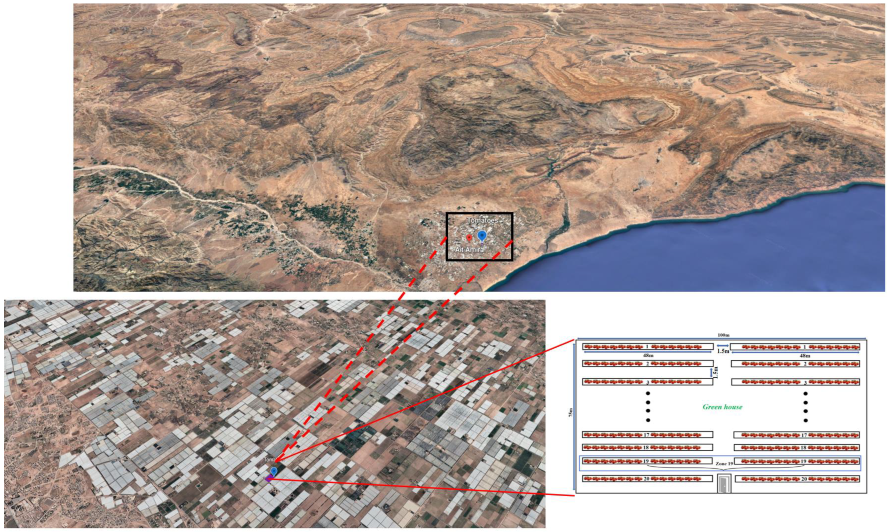
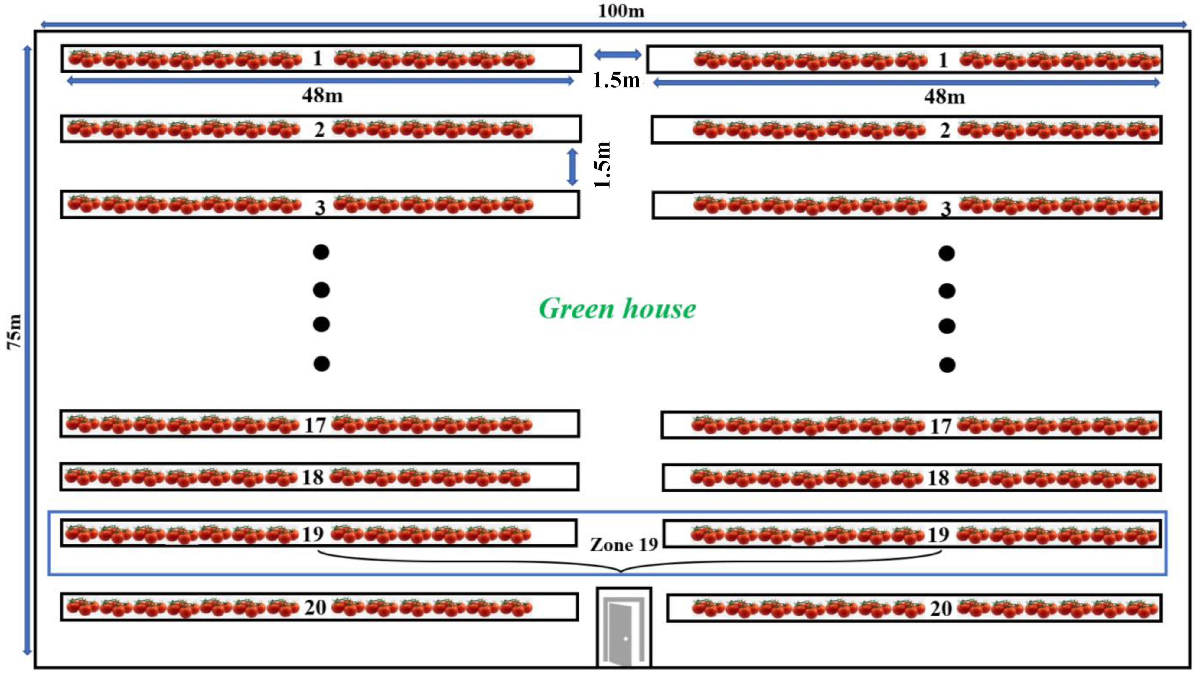
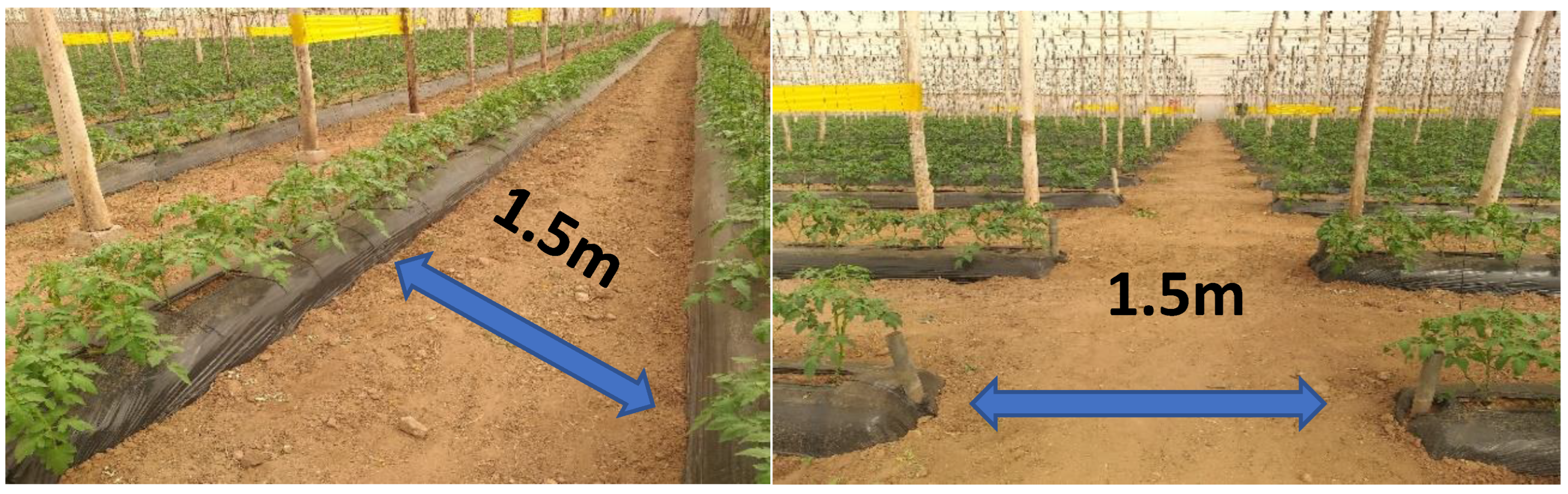
The greenhouse farm used in our study is located in the Ait Aamira region near Agadir. This region is known by the high production of tomatoes and closed greenhouses instead of open fields. The greenhouses studied in our research are located at 30°09′13″ N 9°30′50″ W. Figure 1 shows the greenhouses to be studied. The structure of the greenhouse is based on a plastic cover. The greenhouse studied in this research is divided into 20 regions. Each region contains two tomato rows with 100 m width and 75 m length with a 1.5 m between the rows. In addition, each region is divided in two rows, one with 48 m and the other with 48 m. Figure 2 shows the greenhouse structure and Figure 3 shows real images of the closed greenhouse used in this study.
The study was conducted on the totality of the rows to build a general report of tomato plant’s condition. The tool used for the data collection based on the Parrot Sequoia + multispectral camera. The idea here is to monitor each plant based on the precise GPS coordination of the multispectral camera to deliver an accurate plant assessment that gives each plant its index value and GPS coordinates afterward. The use of these coordinates will help to determine which plant lacks fertilizer, water, or vegetation in a precise approach. In addition, this type of camera gives images separated into four bands, red, green, near-infrared, and RedEdge, with a resolution of 1280 × 960 pixels for each image with a high-resolution to visualize the plants. This gives the flexibility to keep just the RGB image delivered and remove the other unused bands.
2.2. System Modelling
From the literature study, we can conclude that we have three tools for algorithm validation. The first tool is the satellite, the second is the drones, and the third is the ground robots. These three tools aim to support the different sensors that collect, process, and sometimes make real-time decisions. In the case of the satellite, we cannot make decisions simultaneously, and the low resolution of the images causes a wrong diagnosis. For this reason, these solutions are limited to medium and high agricultural fields. Additionally, the application side is limited because the images cannot help when applying counting algorithms, weed detection, and different diseases. So, we are limited to two solutions in our case, either the drones or the soil robots. Unmanned aerial vehicles have shown solid and efficient solutions for surveillance and different applications. However, the problem with these tools is the battery’s autonomy, which does not reach 30 min of flight if no overload has been applied. On the other hand, if we want to build a decision system using a UAV (Unmanned Arial Vehicle), this will increase the weight, affecting the flight time. Similarly, UAVs are not flexible when we want to use surveillance in closed greenhouses. These constraints make the ground robots very strong regarding accuracy and flexibility of applications in open and closed fields such as greenhouses. For this study, we will focus on designing a platform consisting of a soil robot that moves autonomously to monitor vegetation, water, nitrogen, and different applications, such as counting and weed detection. It can also make decisions in real-time. This research aims to show our proposed algorithms’ applicability and utility. In this context, we have developed a system named VSSAgri (vegetation surveillance system for Precision agriculture application). This robot aims to validate the monitoring algorithms proposed in this work. The proposed prototype is based on an embedded architecture and electrical motors powered by a battery. Similarly, it offers a low-cost solution compared to the proposed in the literature.
The proposed system validation has been designed through several steps. Among these steps is the system modeling on CATIA software to study the functional aspect before the hardware design. As for the electrical part, we used Proteus for the functional electrical diagram of the system. In this framework, the system is divided into two parts. The electrical part consists of electric motors and a 12 V battery. The second part is based on the mechanical modeling of the different components.
2.2.1. Mechanical Study
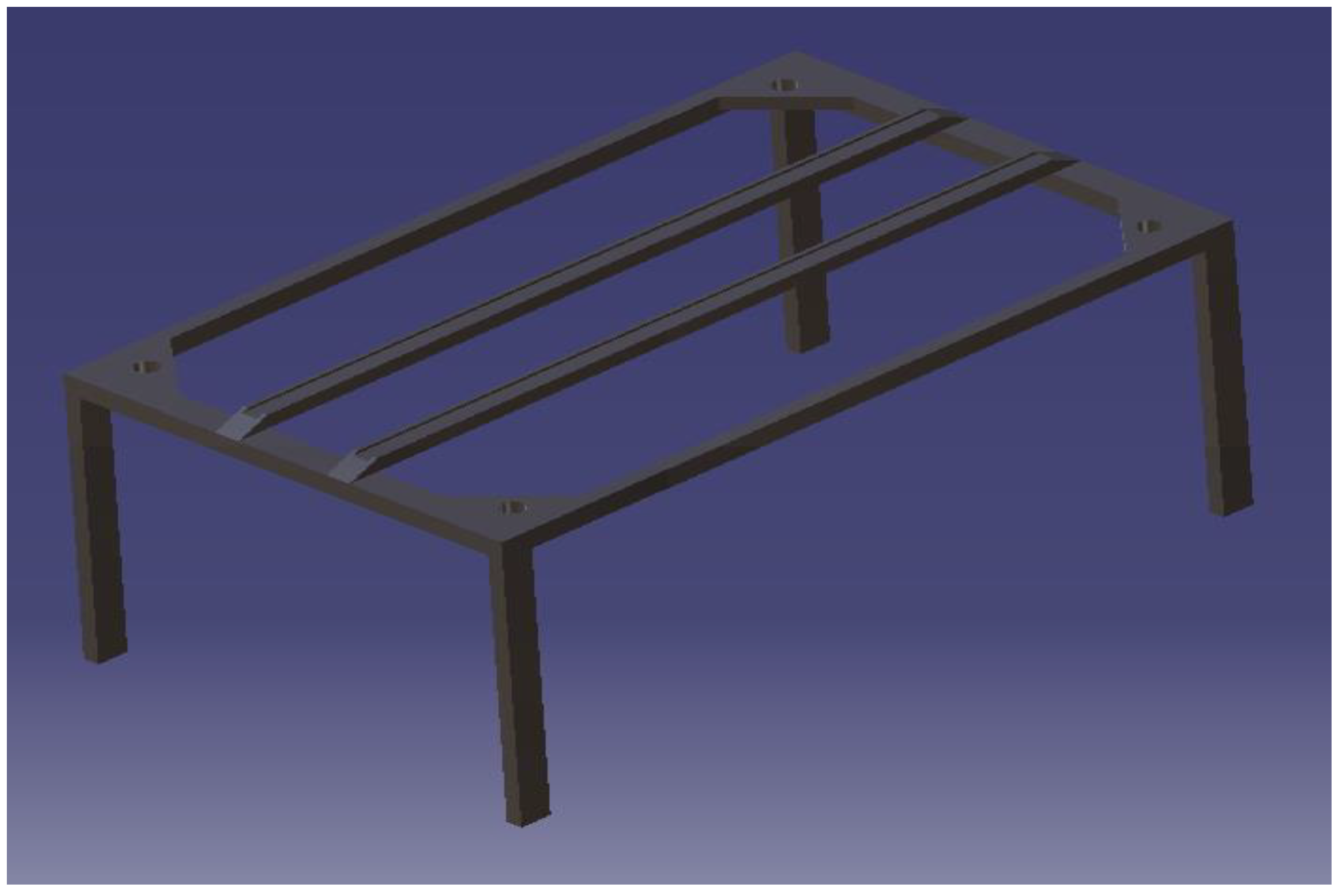
The proposed system consists of metal support with a length of 150 cm and 65 cm wide. The dimensions chosen in our case are based on the test we performed to validate the system. In the real case, either in a greenhouse or an open field, we can change the dimensions of the system. Figure 4 shows the metal support used in our case.
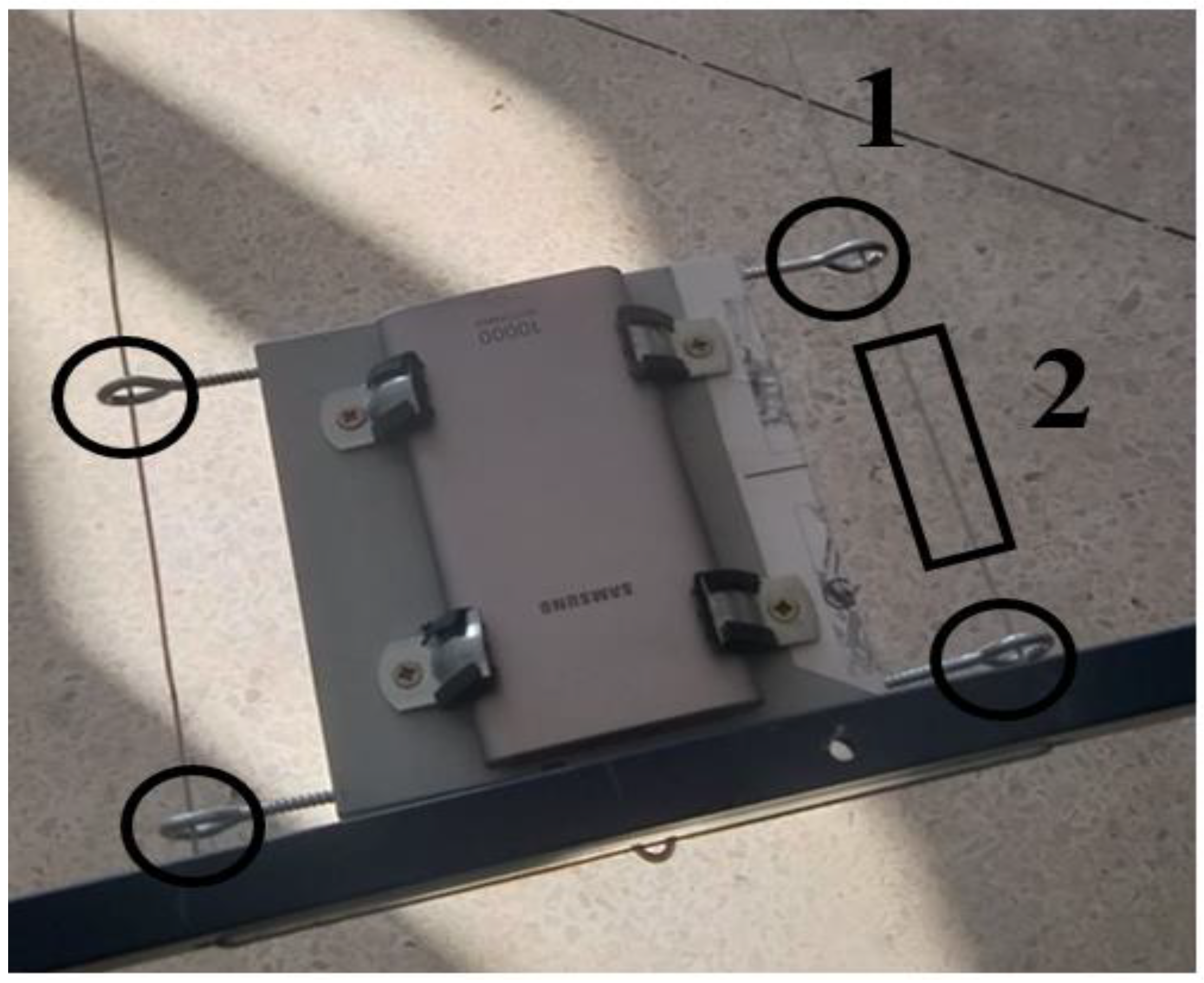
This support is equipped with two barriers in the extremities. The role of these barriers is to guarantee the flow of the processing system. These barriers will support the box that contains the RGB camera, multispectral, and the embedded architecture. In this context, we have tested several solutions based on just two cables that will ensure movement. But the problem of these cables is the movement of the box that influences the speed of displacement due to friction. Figure 5 shows the solution that was proposed before the two barriers.
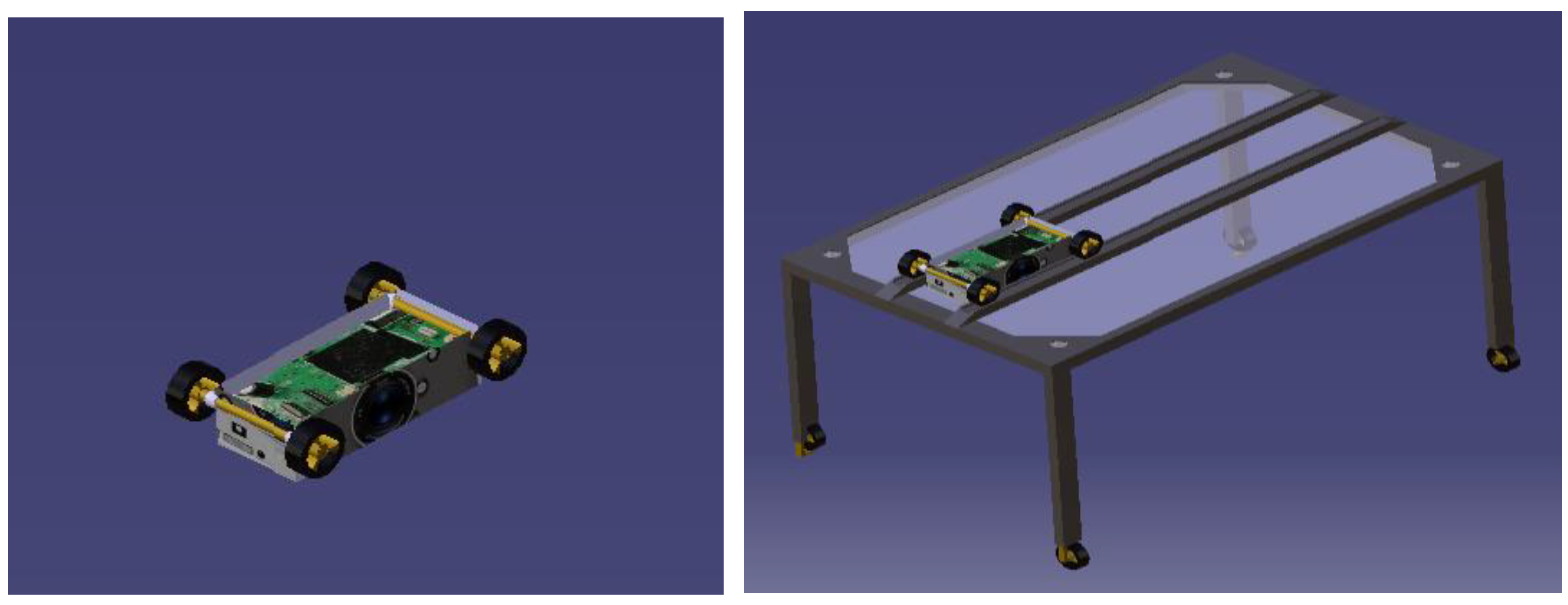
As shown in Figure 5, we have two metal cables in the extremity of the support. This solution has shown some constraints, such as the friction of the box during the displacement. For this reason, we have selected the use of barriers. Then, we have a metal box that consists of a power bank for the power supply of the embedded architecture, and this box carries the different cameras used. As a second solution, we proposed the use of wheels with electric motors for the movement in the two barriers. Figure 6 shows the box used.
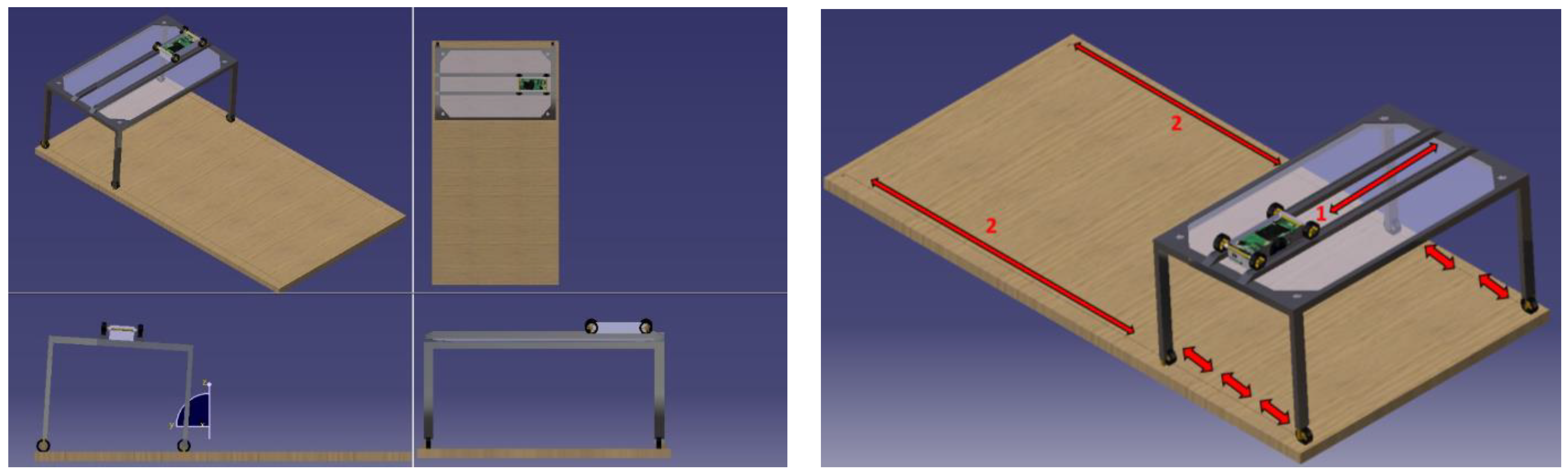
Additionally, we used eight wheels with electric motors, four to drive horizontally, and the others to drive vertically the box’s support. These wheels will realize a scanner principle with a horizontal and vertical displacement to guarantee a general vision of the field that will be handled. The wheels used can be changed if we have problems of movement related to the geography of the agricultural areas. For some applications, we need big wheels that will ensure movement without problems. The collection of all these components will give a complete system, as shown in Figure 7 with the different views on the CATIA software.
Generally, the system moves in a horizontal direction from the box that contains the cameras and the embedded architecture, as shown in Figure 7. Displacement 1 guarantees that the box will cross the horizontal axis to process all the plants in this row. Likewise, displacement 2 ensures the movement of all the support on the fields to move to the second row. These two mechanisms ensure the processing of the whole field. In this case, the temporal constraint is the plants’ real-time indices processing to avoid data loss. This temporal constraint depends on the type of camera that will be used. If we want to monitor indices, such as NDVI, NDWI, and NDRE, we will need a multispectral camera with a timelapse of 5 frames/s. For monitoring the RGB indices, we will need an RGB camera with a timelapse of 30 frames per second, and for all applications, such as plant counting, weed, and disease detection. Temporal constraints in this case have been studied [5,25] based on the different embedded architectures, either CPU-GPU or CPU-FPGA.
2.2.2. Electrical Study
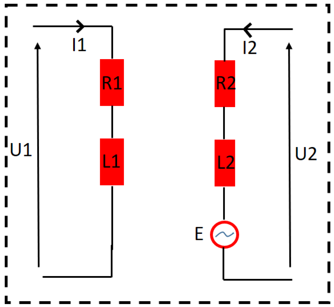
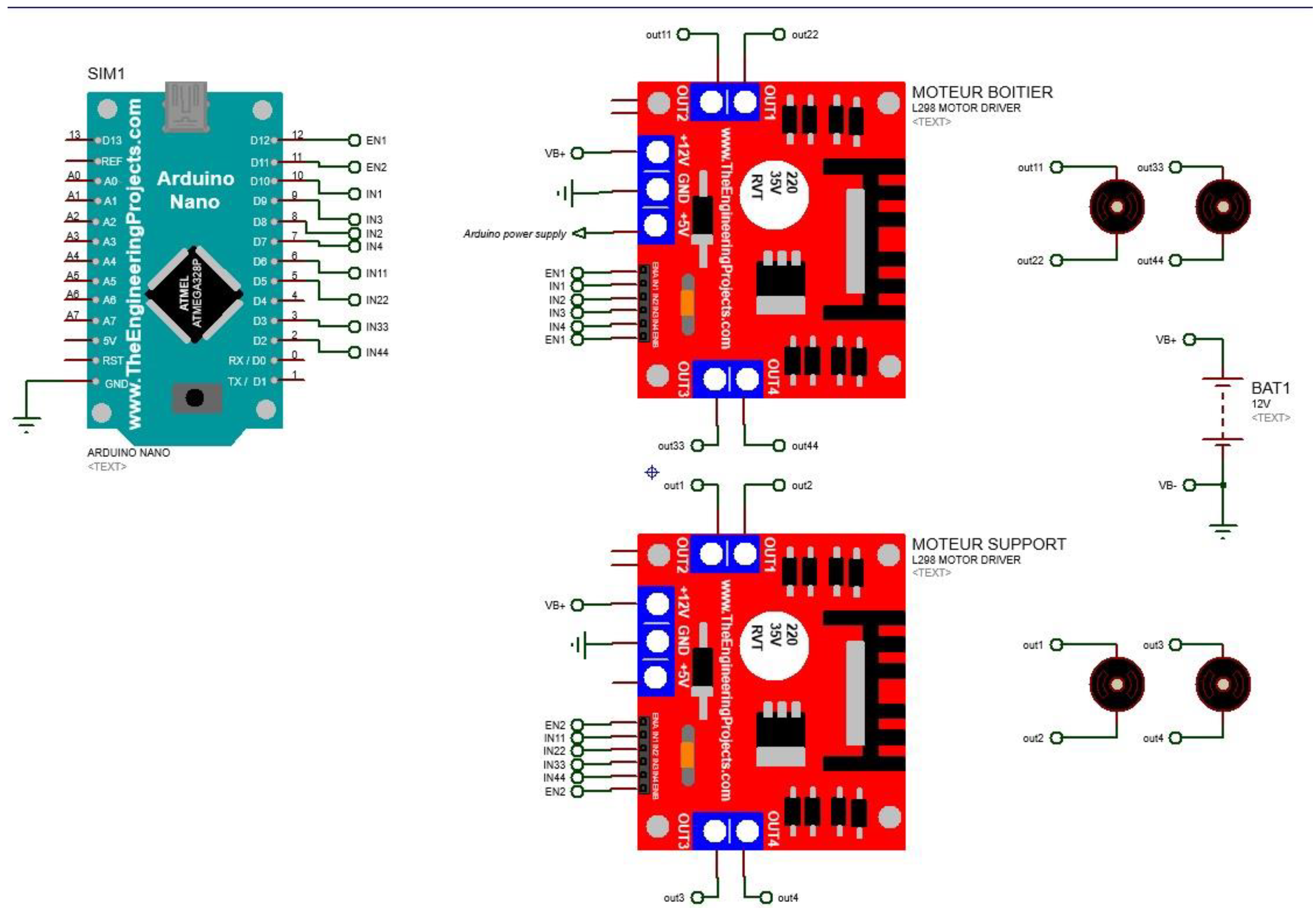
This section focuses on the electrical design of our system. It is equipped with eight electrical motors of low energy consumption. These motors are powered by a 12 V battery that delivers the necessary voltage and current for the system to operate. Four motors are reserved for the movement of all the metal supports, and the others for the movement of the robot. The motors used in the system are flexible and can rotate in both directions. The fundamental design of a DC machine is described by Equations (4)–(7) and Figure 8:
![Sustainability 14 15539 g008]() with U1 voltage of supply field winding, Rs resistance of supply field winding, L1 inductance of field coil, I1 current of supply field winding.
with U2 voltage of armature coil, R2 Resistance of armature coil, I2 current of armature coil, ω angular speed of the motor MSR mutual inductance.
with M2 moment of load, M1 moment of conversion, J total engine, B coefficient of friction.
with U1 voltage of supply field winding, Rs resistance of supply field winding, L1 inductance of field coil, I1 current of supply field winding.
with U2 voltage of armature coil, R2 Resistance of armature coil, I2 current of armature coil, ω angular speed of the motor MSR mutual inductance.
with M2 moment of load, M1 moment of conversion, J total engine, B coefficient of friction.
Figure 8.
Electrical DC machine diagram.

The control of the motors was based on a low-cost Arduino Nano board, and we used only two boards for the driver’s motor. The first will control the support motor and the other for the box. These drivers allow us to synchronize all the motors to ensure a simultaneous movement of the support and the box. The role of the Arduino board is to control the motors through the drivers. Figure 9 shows the electrical diagram of our system.
2.2.3. Algorithm Study
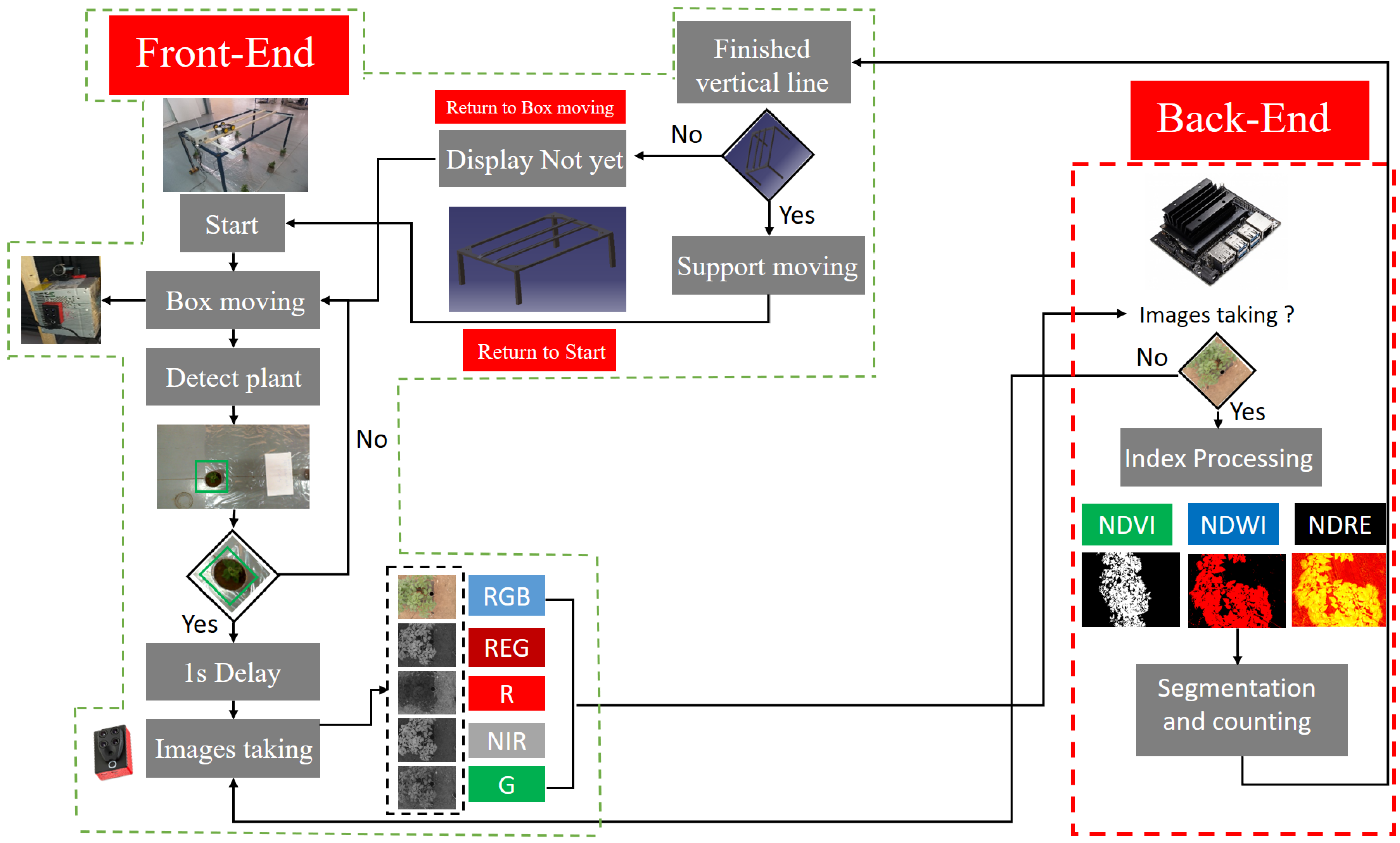
Our proposed algorithm is based on two parts. The first one is for the front end, which controls the autonomous movement of the robot. On the other side, we have the back-end part, which focuses on processing the indices and counting the plants with the suitable threshold. Figure 10 shows the proposed global algorithm.
The algorithm proposed in Figure 10 is based on the autonomous robot movement control and indices processing. The front-end part ensures the movement of the different parts of the robot based on an Arduino board, electric motors, and drivers. The algorithm starts with the box movement, this box contains the embedded architecture that will process, the multispectral and RGB cameras. We used a power bank for the power supply part of the box. On the other hand, the movement control part contains a large battery with 12 V. After the box movement, the vision system detects if we have a plant or not, if yes, then it will apply a 1 s delay, allowing the multispectral cameras to take images with different bands for the indices processing. We have chosen a 1 s delay, depending on our camera’s time-laps (5 frames/s). If not, the system will move the box again to find the plant. For the displacement time, it depends on the distance between the plants. For example, if we have plants one after the other, therefore, every second, we will have five images. In the opposite case, the time to take a new image depends on the distance between the plants. In the case of having located the plant, the multispectral camera takes images with several bands in order to extract useful information. As soon as the images are ready, the system sends them to the back-end to process the indices. The algorithmic part of the index calculation has been studied recently [5,25]. Algorithm 1 shows the front-end process.
| Algorithm 1: Front-End |
 |
On the other hand, for the back-end part, a plant counting algorithm based on classification has been added to count the number of plants that have a low or high index in order to have a general overview. Once the indices are calculated, the algorithm sends the data for segmentation and counting. For the indices processing, we performed a segmentation step that will eliminate the negative values that correspond to the absence of vegetation (e.g., soil, earth…). The NDVI, NDWI, and NDRE values calculated previously are now between 0 and 1. The closer the value is to 1, the more the index reflects good results. Then, we performed multiple thresholding; we considered the values between 0.2 and 0.3 as being relatively weak, so we assigned them the red color; the values between 0.3 and 0.6 were slightly better, we assigned them the orange color; the values between 0.6 and 0.9 showed a very high level, we assigned them a green color. These different thresholds were performed in order to make the images more interpretable for the farmer. The system allows us to create a file containing the index name and value in the output file. On the other side, a file that contains the images colored for each type of index overall will have four files. One for RGB images, two for NDVI, three for NDWI, and NDRE. Algorithm 2 shows the thresholding operation.
| Algorithm 2: Back-End |
 |
The purpose of the watershed technique is to segment the image. It treats the image as a topographic map based on the intensity of the pixels. We find the semantic segmentation that refers to the process during the program to link each pixel of an image to a particular class label. In our case, the result obtained would be a single class, and all the pixels would belong to the same class so the plants would be treated as a single object. Instance segmentation is identical to semantic segmentation except that it differs from semantic segmentation in the fact that it treats the different objects in the image, several objects of the same class, as distinct entities, which allows us to count the number of objects present in the image. The methodology followed in this last part of the algorithm:
- (a)
- We convert the indices image to HSV (hue, saturation, value).
- (b)
- We create the CV_8U version of our HSV image, then we look for the contours present in the HSV image.
- (c)
- We trace the contours on the original image, this tracing step is divided into two steps:
- a.
- Tracing the markers of the foreground;
- b.
- Tracing the background markers in white;
- c.
- The final image is a superposition of the two tracings a and b.
- (d)
- We perform the segmentation using the OpenCV function “Watershed”; afterwards, we fill the labeled objects with randomly generated colors.
The back-end part is based on image processing and is divided into three functions. The first function is for the pre-processing of the images, the second for the indices processing, and the third for the counting operation. After the algorithm finishes the back-end, it goes back to the front end, then a test if the system has finished the vertical line is applied. If yes, it will move all the metal support. If no, it will move only the box for the next plant.
3. Results and Discussion
Interventionary studies involving animals or humans, and other studies that require ethical approval, must list the authority that provided approval and the corresponding ethical approval code.
3.1. Test and Implementation
The processing test was based on two architectures, the first is a low-cost embedded architecture type Nvidia Jetson Nano and the second is a laptop. Using the Jetson Nano architecture has shown that the processing time is reduced using the CUDA language, and we can achieve real-time processing. It is the same case for the laptop, but the problem here is the portability of our system. Table 1 shows the specification of our used device.
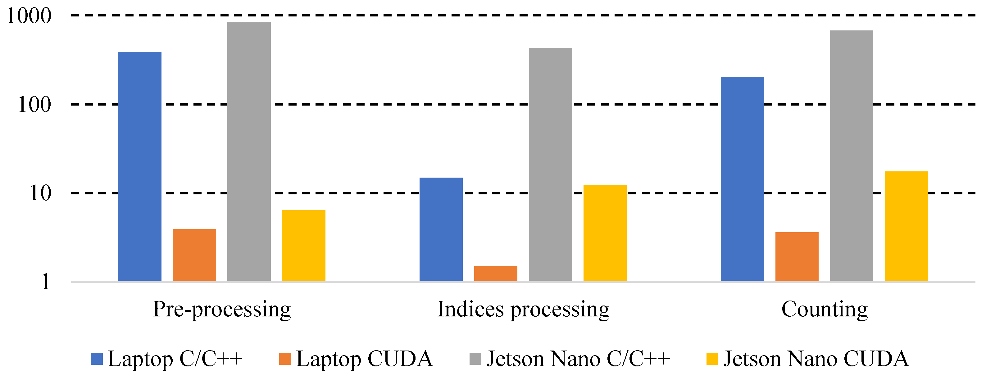
At the first step, a sequential implementation has been proposed in order to study the back-end part of our algorithm. Compared to the Laptop on the Jetson Nano, the three functions constitute the total processing time of the algorithm. Therefore, following a workload analysis based on a hardware/software Co-Design approach allows us to reduce the processing time as much as possible for these three functions for both architectures and mainly for the Jetson Nano. Its compact size of 10 cm × 8 cm × 2.9 cm, and its minimal power consumption of 5 W, added to its limited resources and adapted memory capacity. Its relatively low cost allows it to meet a constraining specification related to embedded systems. After the sequential implementation we based on the CUDA parallel programming language to accelerate the processing. Figure 11 shows a sequential implementation based on C/C++.
In Figure 11, we can conclude that in the laptop, the pre-processing part occupies more than 64% of the processing time, while in the Jetson Nano architecture, we have only 42%. After the time analysis, we decided to accelerate the three functions to decrease the processing time to satisfy the real-time constraint. Table 2 shows a processing time comparison on the laptop and Jetson Nano based on C/C++ and CUDA.
Using the results of the performance profiler, we have gone from a processing time equal to 387.7 ms for the pre-processing to 3.9 ms, which is an acceleration of almost 100 times. For the indices processing, we have an acceleration of 10, and, finally, the counting has been accelerated by 56 times. For the heterogeneous embedded system Jetson Nano, we have gone from a processing time equal to 833.4 ms for the pre-processing to 6.4 ms, an acceleration of 130 times has been achieved. For the second function, we have gone from 432.1 ms to 12.4 ms, equivalent to an acceleration of 34 times, and, finally, the counting has been accelerated by a value of 38 times. Figure 12 represents a temporal synthesis of the different functions on our Laptop and on Jetson Nano.
After the processing time analysis and acceleration, we added a detailed study on memory consumption and processing time. The analysis results obtained have been based on the profiler proposed by Nvidia. The tool offered us the percentage of time that these functions take compared to the global activity level of the GPU of the functions “CUDA memcpy H_to_D” and “CUDA memcpy D_to_H”. Table 3 shows a summary of the results obtained.
Table 3 shows that in the case of the Laptop we have a CPU→GPU transfer rate equal to 2.4829 GB/s and a GPU→CPU rate equal to 2.7274 GB/s. The Jetson Nano embedded system has values 3 times lower in the order of MB/s. Our system consists of two movements, the first for the box containing the embedded architecture and the cameras used for processing. The second part focuses on moving all metal supports to a new row. With this method, we can ensure that all the plants will be processed. Figure 13 shows an overview of our system.
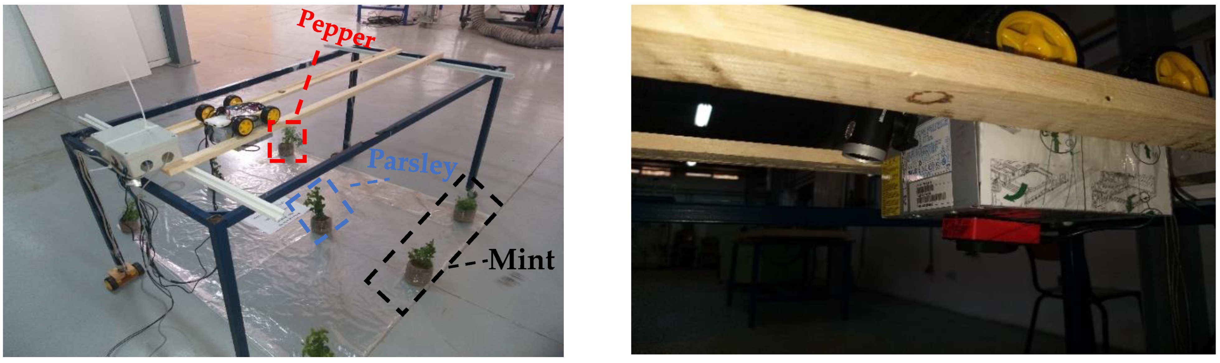
The first step that was performed was the testing and validating of our robot in a closed space based on three rows to validate the mechanism of our system. each rows contain mint, parsley and pepper plant, respectively. The validation of this system in a closed space does not imply accurate functionality in a real environment. For this reason, we have opted after the validation to make a real test in order to validate our algorithmic and systematic approach. In Figure 13, we have on the top left the developed robot and, on the bottom, a multispectral and RGB camera view. In the bottom right image, we have the box that contains the Arduino architecture that operates the movement part of our robot. Figure 14 shows images collected by our robot.
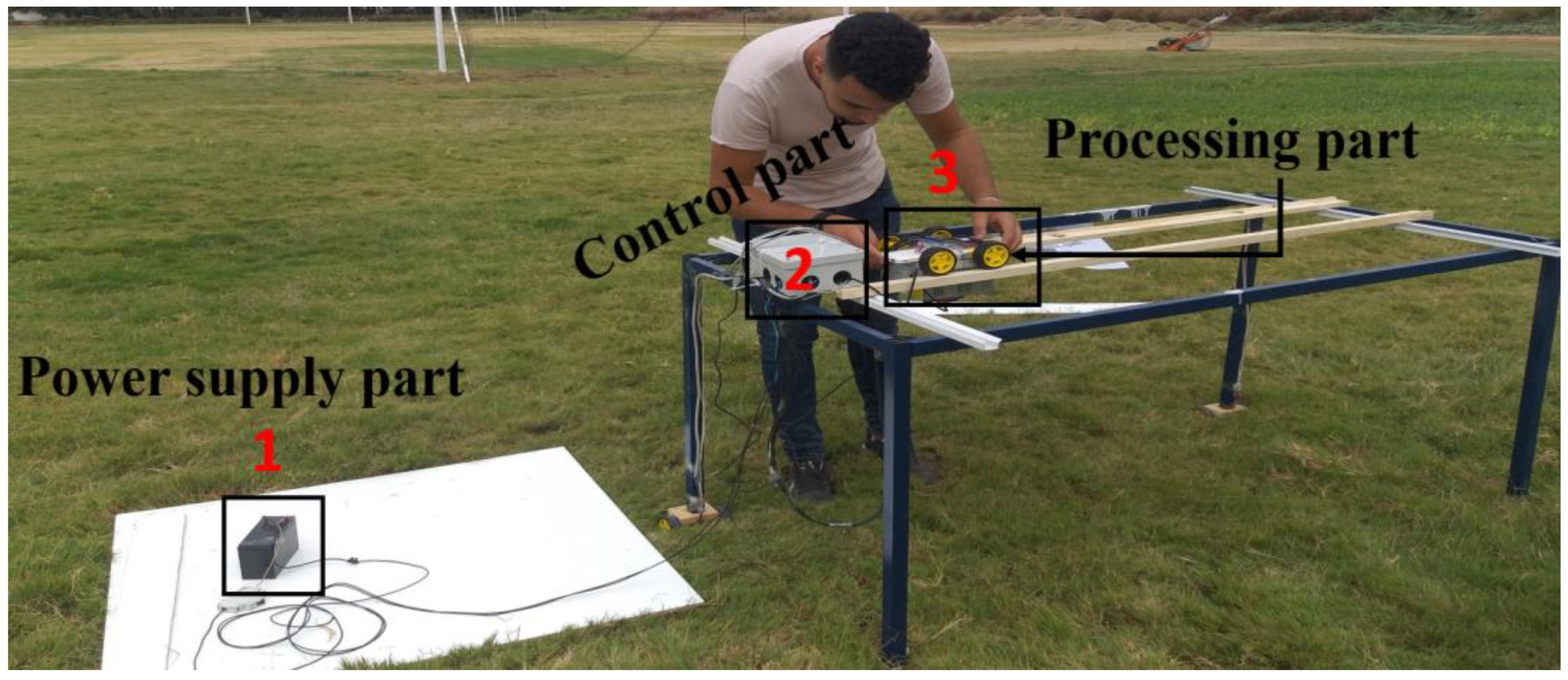
After the prototype validation in the laboratory, we moved to the field validation to evaluate the prototype performance. The results showed that the prototype works in the same conditions and mechanism as in the laboratory. The test was conducted in an open field and a closed greenhouse, showing our system’s flexibility. In addition, our robot can be adapted for the different precision agriculture applications by editing the back-end with the appropriate algorithm. These applications can be either weed detection, fruit and plant counting, or disease detection. In addition, a decision-making system can be added to take real-time actions in the agricultural field. This approach will help the farmer make precise and fast decisions to avoid difficult problems. The developed system is characterized by its low cost and low energy consumption. Figure 15 shows the test of our system in a real agricultural field.
In Figure 15, module 1 represents the battery that powers the motors. On the other hand, we have used a power bank for the power supply of the camera, and for the embedded architecture. Module 2 is a box with the control part that gives actions to the motor. Module 3 is the robot embedding cameras and the architecture-based processing. Additionally, we added a power consumption analysis as part of the robot specifications study. Figure 16 shows the results obtained.
In Figure 16, we have measured the current consumption of the electric motors and the power. We tried to make several iterations to see each time the consumption. The maximum power consumption is about 2.9 W, and for the current consumption is 0.59 A.
3.2. Experimental Result
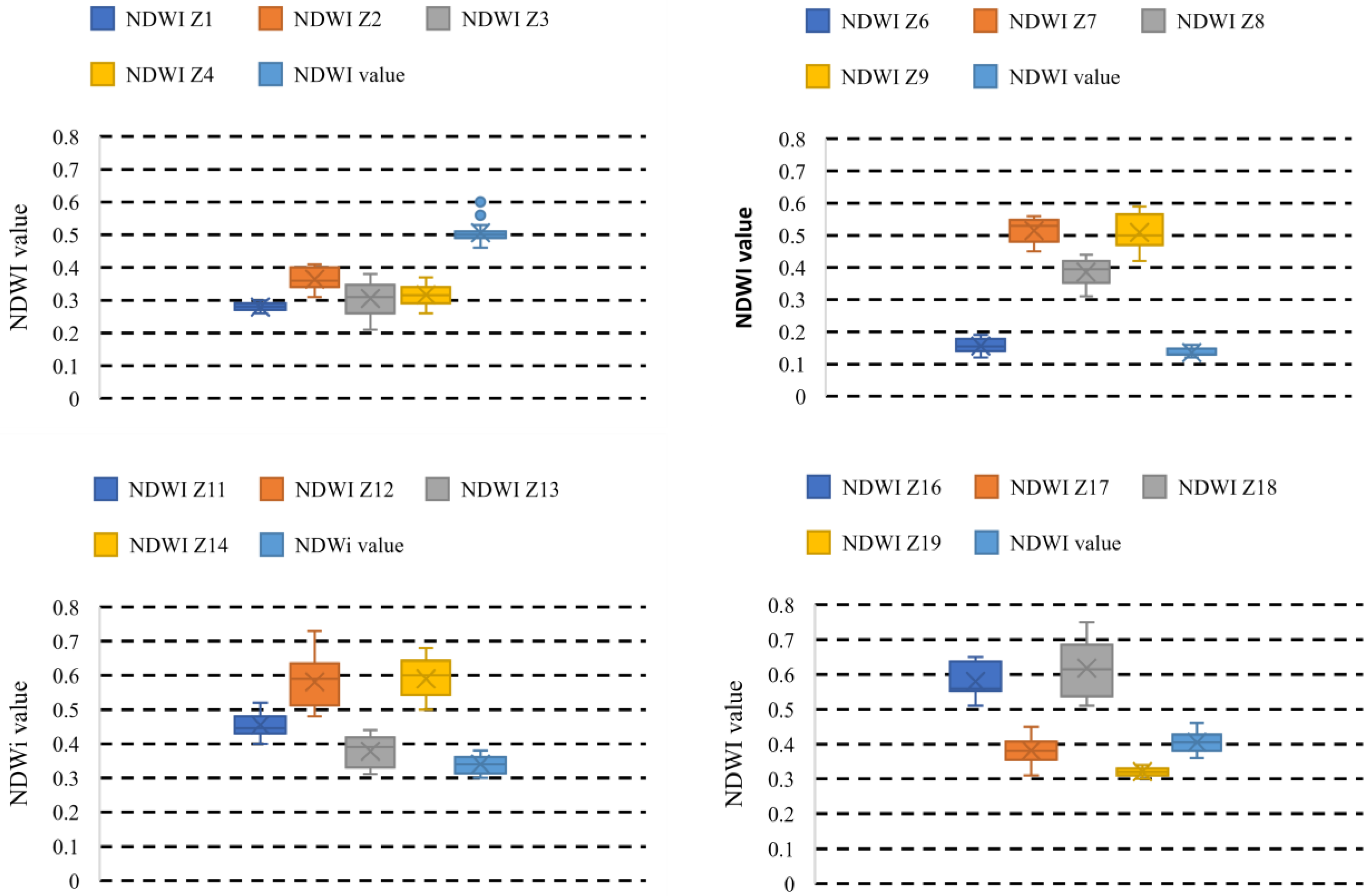
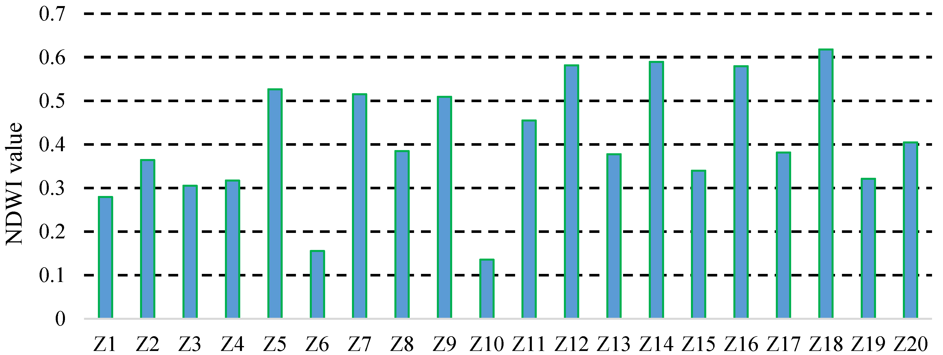
The approach used in this work was based on evaluating several indices, namely NDVI, NDWI, and NDRE. Then, these indices will be collected on all 20 zones to determine the region with low indices. Afterward, we try to determine the GPS coordinates of each region with its index. The first index that has been calculated is NDVI. Figure 17 shows the evaluation of NDVI in the 20 zones.
The NDVI processing was based on several plants to evaluate the variation of this index. The indices’ values vary between 0.15 and 0.8. Generally, the values close to 1 present strong vegetation (reflects that the plant has no problem at the vegetation level). Once we have calculated the variation of NDVI on several plants in the different regions, we move to calculate the NDVI average in each region to define the regions with less vegetation. This method will allow us to locate the regions with vegetation problems. Figure 18 shows the average NDVI in each region.
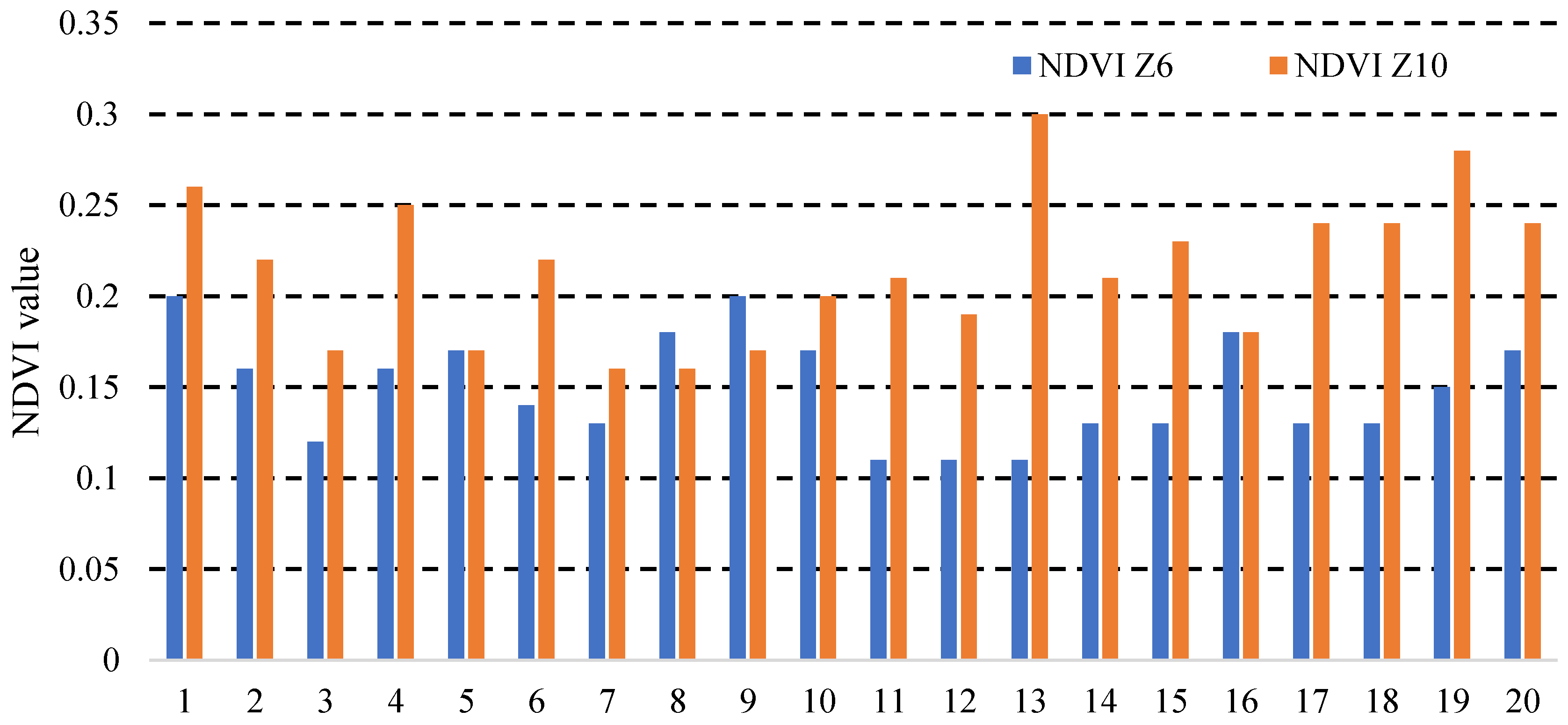
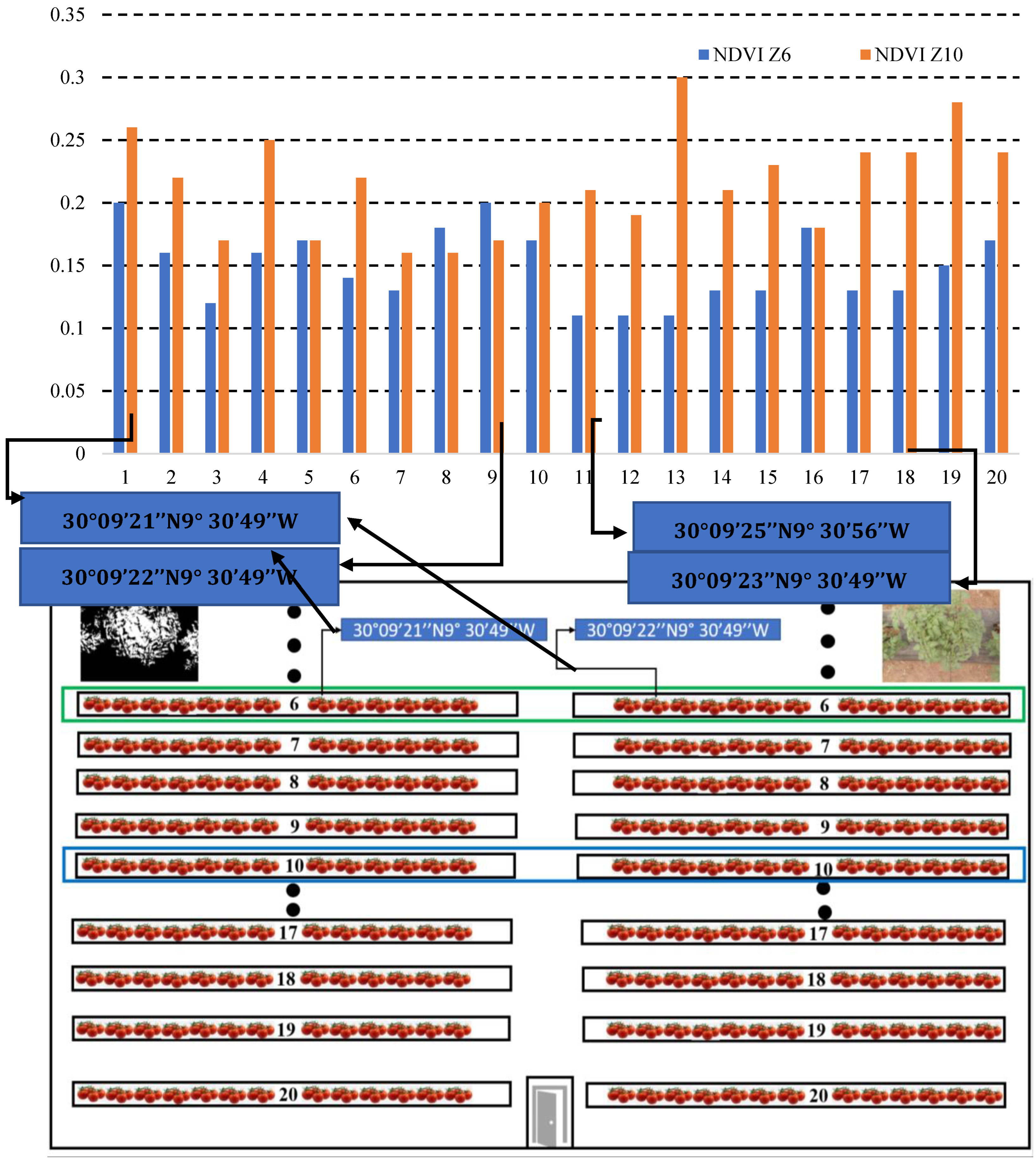
The results in Figure 18 show that zones 6 and 10 give a low index compared to the other zones. Usually, the mean values vary between 0.15 for zone 6 and 0.67 for zone 9. Zones 6 and 10 present low values due to the supply system of the necessary plant components. This reflects the strong relationship between vegetation, water, and the nitrogen content in the plants. After locating the region with a low index, we tried to locate the plants with the vegetation index. Figure 19 shows the vegetation index calculated for each plant.
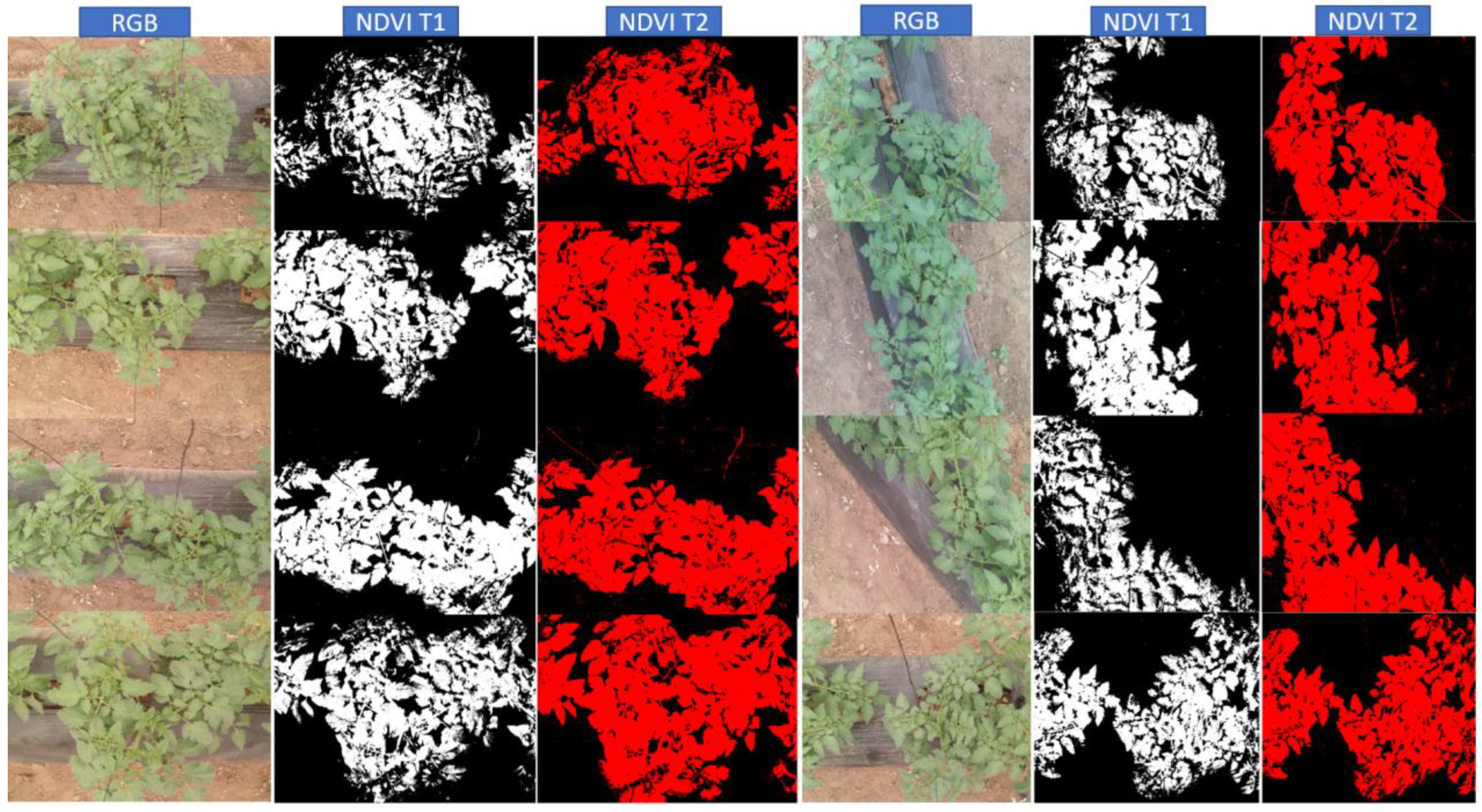
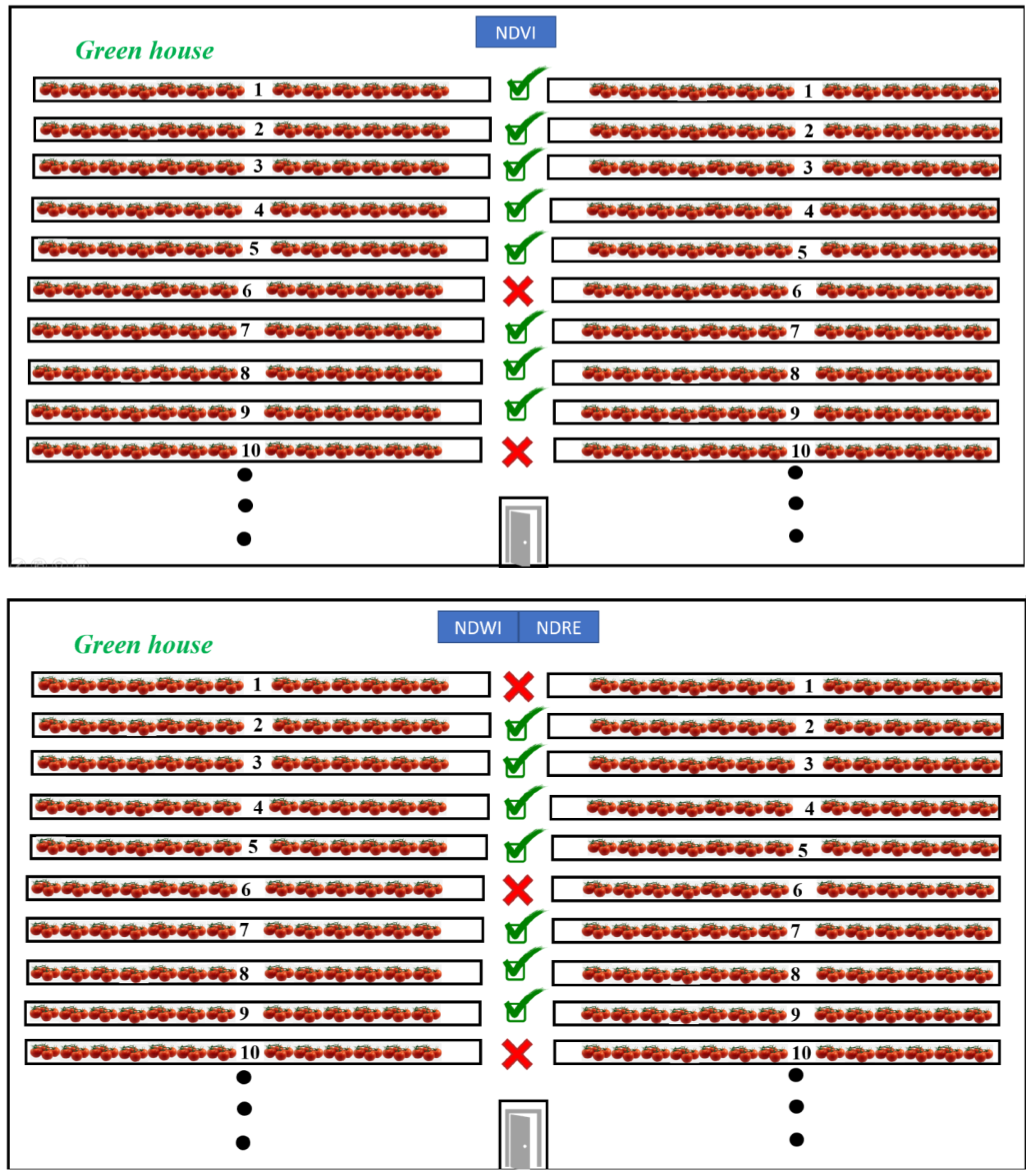
As a result of evaluating the different plants in the areas with a vegetation problem, we determined the plant’s exact position through the images collected with the precise GPS data of the Parrot Sequoia + camera. This localization gives us the plant where we have the vegetation problem, which will help the farmer or robots make precise decisions. Figure 20 shows images of the plants and their NDVI results. In Figure 20 are the RGB images of tomato plants collected in the greenhouse, and we have the evaluation of the binarized NDVI index using the threshold T1 = 0.5. Additionally, we have tried to vary the threshold for the red images with T2 = 0.4. This threshold variation shows the plants that have an index more than T1 or T2. This operation will help us to classify the final results. To determine the index with its proposed threshold, we need to take the plants of each type and create a test with the vegetation sensors afterward to provide each plant with its own index for decision-making.
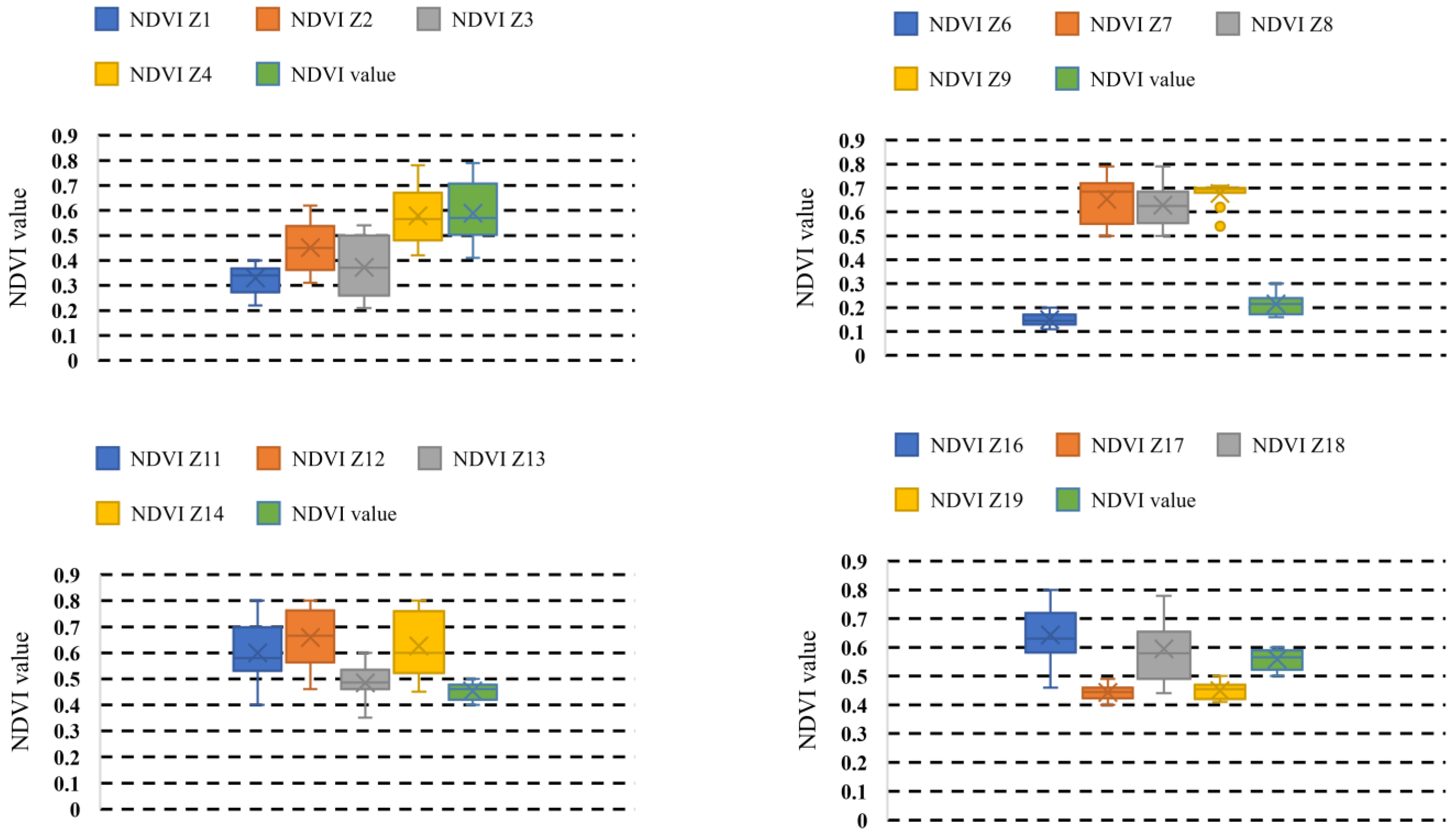
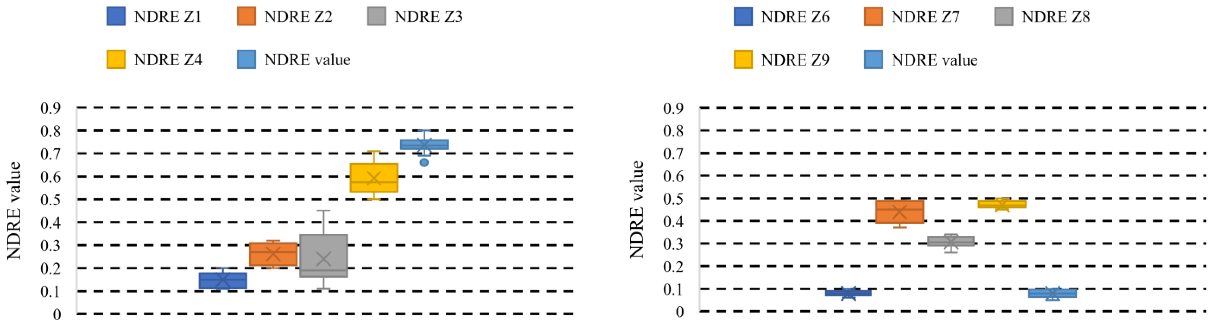
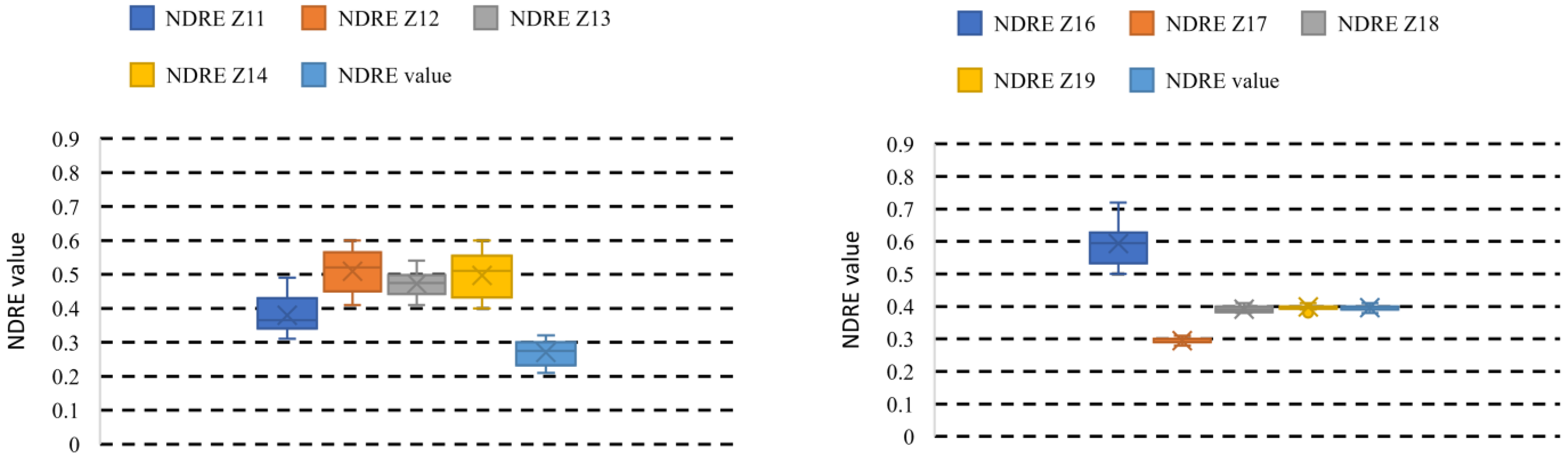
After determining the NDVI vegetation index, we need to calculate the other indices, such as NDRE and NDWI. The reason for calculating these indices is that vegetation is not enough to indicate that the plant is in good condition. The second evaluation was based on the NDRE index shown in Figure 21. The NDRE evaluation was based on a 0.2 threshold. Regions with an index lower than 0.2 suffer from a nitrogen deficiency in the plants. Figure 21 summarizes the results obtained for 20 zones that have been evaluated. The results show that the index varies between 0.079 and 0.75 in zones 10 and 5, with minimum and maximum values. We also find zones 1 and 6 with NDRE values of 0.15 and 0.08. These regions reflect the nitrogen lack in plants. Similarly, for the vegetation index, we have zone 6 and 10 that are in the same situation. On the other hand, in the evaluation of NDRE, another zone that suffers from a lack of nitrogen has been added. After a first synthesis, we concluded that the suffering zones are 6, 1, and 10. For this reason, it is necessary to extend the evaluation and see the average of the NDRE index in the different regions. Figure 22 shows the different areas’ evaluation based on each zone’s average.
The application of the average processing in the different zones has reinforced the synthesis elaborated in Figure 22. It also confirmed that zones 6, 1, and 10 suffer from the lack of nitrogen. Our evaluation methodology based on a thorough evaluation that aims to determine the exact plants where we have problems.
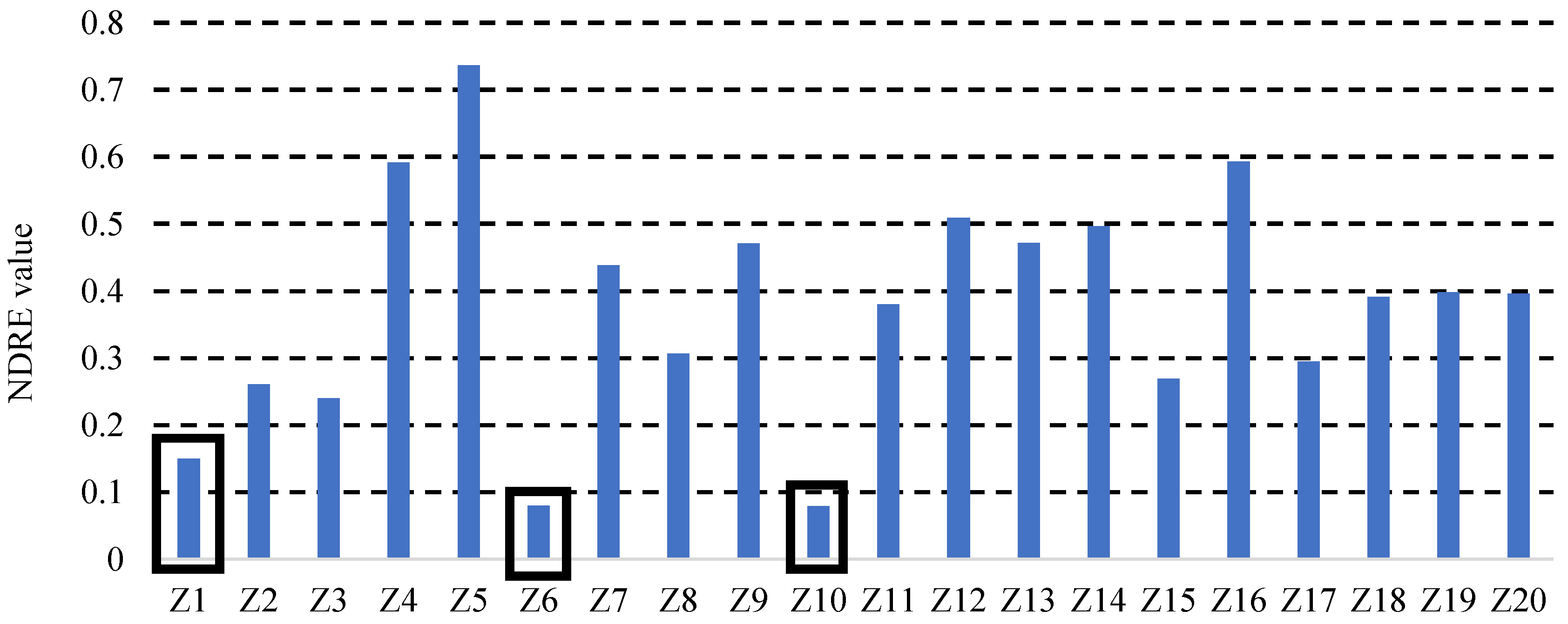
In Figure 23, we have shown an evaluation of 20 plants in regions 1, 6, and 10. The results show that the plants in regions 6 and 10 have very low values compared to zone 1. The values vary between 0.05 and 0.1. On the other hand, zone 1 varies between 0.2 and 0.11. After evaluating the different plants, it is necessary to determine the precise localization of the plants. The third vital index that is opted for our evaluation is NDWI. This index determines the amount of water in the vegetation. Figure 24 shows the evaluation of the NDWI.
The NDWI evaluation is based on a threshold of 0.3. Areas with less than 0.3 have a water deficiency or water absence, while areas with more than 0.3 have water. The index evaluation showed that, like the NDRE, areas 1, 6, and 10 have low water content. Figure 25 and Figure 26 present the results in each zone.
The NDWI values in Figure 26 range from 0.618 to 0.13 for zones 18 and 10. The calculation of NDWI in the figure is based on the average of each zone. The global analysis of the greenhouse study showed that vegetation problems appeared in zones 6 and 10, while water and nitrogen problems appeared in zones 1, 6, and 10. This methodology of interpretation and this study will help farmers monitor the agricultural fields and determine the plants and areas that suffer from a various problem. This will increase the productivity of the farm. After processing the indices in each plant, we will have the precise localization of each plant Figure 27 shows an example of NDVI.
The GPS data shown in Figure 28 are provided by the Parrot Sequoia + camera. Then, we generated a map of the greenhouse with the 20 zones and the index result with the GPS data, as shown in Figure 27. This will improve the decision system associated with the closed greenhouse. Therefore, in the map, the green and blue colored rectangle shows zones 10 and 6. Additionally, the GPS coordinates of the plants that have a vegetation problem. After evaluating the different vital indices, including NDVI, NDRE, and NDWI, we obtained the different information needed in the agricultural fields. This information is the most relevant to have an overview of the health of the plants. As soon as the evaluation is finished, a global map should be generated for the farmer, containing the different information about the greenhouse. Figure 28 shows the overall map of the indices monitoring.
The GPS data shown in Figure 28 are provided by the Parrot Sequoia + camera. Then, we can generate a map of the greenhouse with the 20 zones and the index result with the GPS data, as shown in Figure 27. This will improve the decision system associated with the closed greenhouse. In the map, the green and blue colored rectangle shows these zones 10 and 6.
In addition, the GPS coordinates of the plants that have a vegetation problem are given. After evaluating the different vital indices, including NDVI, NDRE, and NDWI, we obtained the different information needed in the agricultural fields. This information is the most relevant to have an overview of the health of the plants. As soon as the evaluation is finished, a global map should be generated for the farmer, containing the different information about the greenhouse. Figure 28 shows the overall map of the indices monitoring. Table 4 shows a Summary of normalized indices results in the closed greenhouse.
4. Conclusions
The validation of the algorithmic approach is a very important step to test the algorithm’s reliability. In real scenarios, we can find a variety of environmental problems that influence the algorithm’s operation. The development of autonomous robots helps to validate the research approach and make it useful. In this work, we have proposed an autonomous monitoring system that monitors crops in closed greenhouses and in open fields. This system delivers a map that contains an image with vegetation, water, and fertilizer information, and GPS localization. This technique will increase the precision of monitoring, which will help us to improve the decision systems and reduce the consumption of resources required by the plant for growth. This will maximize the yield by decreasing the consumption of resources. Therefore, we added a sequential and parallel implementation in a heterogeneous embedded architecture type CPU-GPU in order to study the processing time and the memory consumption. The results allowed us to process each image in 1.94 s for the Jetson Nano embedded architecture. On the other hand, the Laptop processed each image in 0.604 s, which does not give real-time processing based on 5 images/s. For this reason, an optimization based on the architecture-algorithm mapping approach allowed us to reduce the processing time for the Laptop to 9 ms and the embedded architecture to 36 ms. This gave us real-time processing for both architectures with an acceleration factor of 66 for the laptop and 54 for the Jetson Nano.
Author Contributions
Conceptualization, A.S. writing—original draft preparation, A.S. and A.S.; methodology, A.S. and A.E.O.; software, A.S. and A.E.O.; validation, M.E. and F.T.; formal analysis, R.L.; data curation, A.S.; writing—review and editing, M.E. and R.L.; visualization, F.T. All authors have read and agreed to the published version of the manuscript.
Funding
This research is funded by the National Centre for Scientific and Technical Research of Morocco (CNRST) (grant number: 19 UIZ2020).
Institutional Review Board Statement
Not applicable.
Informed Consent Statement
Not applicable.
Data Availability Statement
Data used in this paper are available upon requests.
Acknowledgments
We owe a debt of gratitude to thank the National Centre for Scientific and Technical Research of Morocco (CNRST) for their financial support and for their supervision (grant number: 19 UIZ2020).
Conflicts of Interest
The authors declare no conflict of interest.
References
- Wang, T.; Chen, B.; Zhang, Z.; Li, H.; Zhang, M. Applications of machine vision in agricultural robot navigation: A review. Comput. Electron. Agric. 2022, 198, 107085. [Google Scholar] [CrossRef]
- Chebrolu, N.; Lottes, P.; Schaefer, A.; Winterhalter, W.; Burgard, W.; Stachniss, C. Agricultural robot dataset for plant classification, localization and mapping on sugar beet fields. Int. J. Robot. Res. 2017, 36, 1045–1052. [Google Scholar] [CrossRef] [Green Version]
- Abualkishik, A.Z.; Almajed, R.; Thompson, W. Evaluating Smart Agricultural Production Efficiency using Fuzzy MARCOS method. J. Neutrosophic Fuzzy Syst. 2022, 3, 8–18. [Google Scholar] [CrossRef]
- Tofigh, M.A.; Mu, Z. Intelligent Web Information Extraction Model for Agricultural Product Quality and Safety System. J. Intell. Syst. Internet Things 2021, 4, 99–110. [Google Scholar] [CrossRef]
- Saddik, A.; Latif, R.; El Ouardi, A.; Alghamdi, M.I.; Elhoseny, M. Improving Sustainable Vegetation Indices Processing on Low-Cost Architectures. Sustainability 2022, 14, 2521. [Google Scholar] [CrossRef]
- Saddik, A.; Latif, R.; el Ouardi, A.; Elhoseny, M.; Khelifi, A. Computer development based embedded systems in precision agriculture: Tools and application. Acta Agric. Scand. Sect. B Soil Plant Sci. 2022, 72, 589–611. [Google Scholar] [CrossRef]
- Amine, S.; Latif, R.; El Ouardi, A. Low-Power FPGA Architecture Based Monitoring Applications in Precision Agriculture. J. Low Power Electron. Appl. 2021, 11, 39. [Google Scholar] [CrossRef]
- Abualkishik, A.Z.; Almajed, R.; Thompson, W. Multi-attribute decision-making method for prioritizing autonomous vehicles in real-time traffic management: Towards active sustainable transport. Int. J. Wirel. Ad Hoc Commun. 2021, 3, 91–101. [Google Scholar] [CrossRef]
- Devanna, R.P.; Milella, A.; Marani, R.; Garofalo, S.P.; Vivaldi, G.A.; Pascuzzi, S.; Galati, R.; Reina, G. In-Field Automatic Identification of Pomegranates Using a Farmer Robot. Sensors 2022, 22, 5821. [Google Scholar] [CrossRef]
- Skoczeń, M.; Ochman, M.; Spyra, K.; Nikodem, M.; Krata, D.; Panek, M.; Pawłowski, A. Obstacle Detection System for Agricultural Mobile Robot Application Using RGB-D Cameras. Sensors 2021, 21, 5292. [Google Scholar] [CrossRef]
- Kamandar, M.R.; Massah, J.; Jamzad, M. Design and evaluation of hedge trimmer robot. Comput. Electron. Agric. 2022, 199, 107065. [Google Scholar] [CrossRef]
- Zheng, W.; Guo, N.; Zhang, B.; Zhou, J.; Tian, G.; Xiong, Y. Human Grasp Mechanism Understanding, Human-Inspired Grasp Control and Robotic Grasping Planning for Agricultural Robots. Sensors 2022, 22, 5240. [Google Scholar] [CrossRef] [PubMed]
- Li, K.; Huo, Y.; Liu, Y.; Shi, Y.; He, Z.; Cui, Y. Design of a lightweight robotic arm for kiwifruit pollination. Comput. Electron. Agric. 2022, 198, 107114. [Google Scholar] [CrossRef]
- Cho, B.-H.; Kim, Y.-H.; Lee, K.-B.; Hong, Y.-K.; Kim, K.-C. Potential of Snapshot-Type Hyperspectral Imagery Using Support Vector Classifier for the Classification of Tomatoes Maturity. Sensors 2022, 22, 4378. [Google Scholar] [CrossRef] [PubMed]
- Yang, J.; Ni, J.; Li, Y.; Wen, J.; Chen, D. The Intelligent Path Planning System of Agricultural Robot via Reinforcement Learning. Sensors 2022, 22, 4316. [Google Scholar] [CrossRef]
- Gao, P.; Lee, H.; Jeon, C.-W.; Yun, C.; Kim, H.-J.; Wang, W.; Liang, G.; Chen, Y.; Zhang, Z.; Han, X. Improved Position Estimation Algorithm of Agricultural Mobile Robots Based on Multisensor Fusion and Autoencoder Neural Network. Sensors 2022, 22, 1522. [Google Scholar] [CrossRef]
- Yang, T.; Ye, J.; Zhou, S.; Xu, A.; Yin, J. 3D reconstruction method for tree seedlings based on point cloud self-registration. Comput. Electron. Agric. 2022, 200, 107210. [Google Scholar] [CrossRef]
- Duan, M.; Song, X.; Liu, X.; Cui, D.; Zhang, X. Mapping the soil types combining multi-temporal remote sensing data with texture features. Comput. Electron. Agric. 2022, 200, 107230. [Google Scholar] [CrossRef]
- Chghaf, M.; Rodriguez, S.; Ouardi, A.E. Camera, LiDAR and Multi-modal SLAM Systems for Autonomous Ground Vehicles: A Survey. J. Intell. Robot Syst. 2022, 105, 2. [Google Scholar] [CrossRef]
- Nguyen, D.D.; El Ouardi, A.; Rodriguez, S.; Bouaziz, S. FPGA implementation of HOOFR bucketing extractor-based real-time embedded SLAM applications. J. Real-Time Image Proc. 2021, 18, 525–538. [Google Scholar] [CrossRef]
- Ericson, S.K.; Åstrand, B.S. Analysis of two visual odometry systems for use in an agricultural field environment. Biosyst. Eng. 2018, 166, 116–125. [Google Scholar] [CrossRef] [Green Version]
- Weiss, U.; Biber, P. Plant detection and mapping for agricultural robots using a 3D LIDAR sensor. Robot. Auton. Syst. 2011, 59, 265–273. [Google Scholar] [CrossRef]
- Ali, I.; Durmush, A.; Suominen, O.; Yli-Hietanen, J.; Peltonen, S.; Atanas, J.; Finn, G. Forest dataset: A forest landscape for visual SLAM. Robot. Auton. Syst. 2020, 132, 103610. [Google Scholar] [CrossRef]
- Aguiar, A.S.; dos Santos, F.N.; Sobreira, H.; Cunha, J.B.; Sousa, A.J. Particle filter refinement based on clustering procedures for high-dimensional localization and mapping systems. Robot. Auton. Syst. 2021, 137, 103725. [Google Scholar] [CrossRef]
- Saddik, A.; Latif, R.; Elhoseny, M.; El Ouardi, A. Real-time evaluation of different indexes in precision agriculture using a heterogeneous embedded system. Sustain. Comput. Inform. Syst. 2021, 30, 100506. [Google Scholar] [CrossRef]
- Tucker, C.J. Red and photographic infrared linear combinations for monitoring vegetation. Remote Sens. Environ. 1979, 8, 127–150. [Google Scholar] [CrossRef] [Green Version]
- McFeeters, S.K. The use of the Normalized Difference Water Index (NDWI) in the delineation of open water features. Int. J. Remote Sens. 1996, 17, 1425–1432. [Google Scholar] [CrossRef]
Figure 1.
Greenhouse location.

Figure 2.
Greenhouse structure.

Figure 3.
Greenhouse real area.

Figure 4.
Metal support.

Figure 5.
First proposed solution for box movement.

Figure 6.
Box used in our prototype.

Figure 7.
Different views of the prototype using the CATIA software.

Figure 9.
Electrical diagram.

Figure 10.
General algorithm overview.

Figure 11.
Processing time analysis.

Figure 12.
Temporal synthesis of the different functions.

Figure 13.
System overview.


Figure 14.
Camera overview of our system.

Figure 15.
Test and evaluation of the system in real field.

Figure 16.
Power and current consumption of the electric motors.

Figure 17.
NDVI evaluation based on 20 regions.

Figure 18.
NDVI average.

Figure 19.
NDVI of each plant for 20 regions.

Figure 20.
RGB and NDVI image evaluation.

Figure 21.
NDRE evaluation for 20 regions.


Figure 22.
NDRE average.

Figure 23.
NDRE for 1, 6 and 10 zones.

Figure 24.
NDWI evaluation based on 20 regions.

Figure 25.
NDWI average.

Figure 26.
NDWI for 1, 6 and 10 zones.

Figure 27.
NDVI and GPS data for 6 and 10 zones.

Figure 28.
Indices general view.


Table 1.
Architecture specification.
| Device type | Laptop | Nvidia Jetson Nano |
| Processor type | Intel CORE | ARMv8 |
| CPU name | i7-10510U | ARM A57 |
| Base frequency | 1.80 GHz | 1.43 GHz |
| Number of cores | 4 (8 threads) | 4 |
| GPU | GeForce MX250 | Tegra X1 |
| GPU Architecture | Pascal | Maxwell |
| Base frequency | 1519 MHz | 643 MHz |
| Number of cores | 384 | 128 |
| Memory | 16 GB DDR4{XE “CDDR” \t “: Double Data Rate ”} | 4 GB LPDDR4{ XE “LPDDR4” \t “: Low Power Double Data Rate ” } |
Table 2.
Processing time comparison.
| C/C++ (s) | CUDA (s) | Acceleration | |
|---|---|---|---|
| Laptop | |||
| Pre-processing | 0.3878 | 0.0039 | 99.43 |
| Indices processing | 0.0149 | 0.0015 | 9.93 |
| Counting | 0.2021 | 0.0036 | 56.13 |
| Jetson Nano | |||
| Pre-processing | 0.8334 | 0.0064 | 130.21 |
| Indices processing | 0.4321 | 0.0124 | 34.84 |
| Counting | 0.6783 | 0.0175 | 38.76 |
Table 3.
GPU activity and Data workload results.
| GPU Activity (%) | Data Workload | |||
|---|---|---|---|---|
| GeForce MX250 | Jetson | GeForce MX250(GB/s) | Jetson (MB/s) | |
| CUDA memcpy H_to_D | 34.78 | 30.35 | 2.4829 | 761.1025 |
| CUDA memcpy D_to_H | 18.46 | 15.62 | 2.7274 | 803.36 |
| Total | 53.24 | 45.97 | 5.21 | 1564 |
Table 4.
Summary of normalized indices results in the closed greenhouse.
| Nomenclature for Table | |||
|---|---|---|---|
| - | <0.2 | ||
| + | 0.2–0.4 | ||
| ++ | 0.4–0.6 | ||
| +++ | <0.6 | ||
| Zones | Value | ||
| NDVI | NDWI | NDRE | |
| 1 | + | + | - |
| 2 | + | + | + |
| 3 | ++ | + | + |
| 4 | ++ | + | ++ |
| 5 | ++ | ++ | +++ |
| 6 | - | - | - |
| 7 | +++ | ++ | ++ |
| 8 | +++ | + | + |
| 9 | +++ | ++ | ++ |
| 10 | - | - | - |
| 11 | +++ | ++ | + |
| 12 | +++ | ++ | ++ |
| 13 | ++ | + | ++ |
| 14 | +++ | ++ | ++ |
| 15 | ++ | + | + |
| 16 | +++ | ++ | ++ |
| 17 | ++ | + | + |
| 18 | ++ | ++ | + |
| 19 | ++ | + | + |
| 20 | ++ | ++ | + |
Publisher’s Note: MDPI stays neutral with regard to jurisdictional claims in published maps and institutional affiliations. |
© 2022 by the authors. Licensee MDPI, Basel, Switzerland. This article is an open access article distributed under the terms and conditions of the Creative Commons Attribution (CC BY) license (https://creativecommons.org/licenses/by/4.0/).
Share and Cite
MDPI and ACS Style
Saddik, A.; Latif, R.; Taher, F.; El Ouardi, A.; Elhoseny, M. Mapping Agricultural Soil in Greenhouse Using an Autonomous Low-Cost Robot and Precise Monitoring. Sustainability 2022, 14, 15539. https://doi.org/10.3390/su142315539
AMA Style
Saddik A, Latif R, Taher F, El Ouardi A, Elhoseny M. Mapping Agricultural Soil in Greenhouse Using an Autonomous Low-Cost Robot and Precise Monitoring. Sustainability. 2022; 14(23):15539. https://doi.org/10.3390/su142315539
Chicago/Turabian StyleSaddik, Amine, Rachid Latif, Fatma Taher, Abdelhafid El Ouardi, and Mohamed Elhoseny. 2022. "Mapping Agricultural Soil in Greenhouse Using an Autonomous Low-Cost Robot and Precise Monitoring" Sustainability 14, no. 23: 15539. https://doi.org/10.3390/su142315539
Note that from the first issue of 2016, this journal uses article numbers instead of page numbers. See further details here.